Abstract
Data obtained using direct numerical simulations (DNS) of pressure-driven turbulent channel flow are studied in the range 180 10,000. Reynolds number effects on the mean velocity profile (MVP) and second order statistics are analyzed with a view of finding logarithmic behavior in the overlap region or even further from the wall, well in the boundary layer’s outer region. The values of the von Kármán constant for the MVPs and the Townsend–Perry constants for the streamwise and spanwise fluctuation variances are determined for the Reynolds numbers considered. A data-driven model of the MVP, proposed and validated for zero pressure-gradient flow over a flat plate, is employed for pressure-driven channel flow by appropriately adjusting Coles’ strength of the wake function parameter, Π. There is excellent agreement between the analytic model predictions of MVP and the DNS-computed MVP as well as of the Reynolds shear stress profile. The skin friction coefficient Cf is calculated analytically. The agreement between the analytical model predictions and the DNS-based computed discrete values of Cf is excellent.
1. Introduction
The study of wall turbulence is one of the most challenging topics in turbulence research. Theoretical, experimental, and computational approaches encounter insurmountable difficulties, especially in the high Reynolds number regime. However, the great importance of wall turbulence in engineering applications and the challenging nature of the physics involved have maintained a continuous string of efforts to understand, model, and compute such flows.
Fundamental research has focused on several turbulent flows in simple geometries usually referred to as canonical flows. Canonical turbulent flows include turbulent Couette and Poiseuille flows between parallel plates, flows in straight pipes of constant circular cross-section, liquid flows of uniform depth in wide open channels and zero pressure-gradient external flow over a flat plate. The mean flow field in wall-bounded cases (such as flow in channels and pipes) is parallel and the thickness of the boundary layers formed is constant. Furthermore, in planar and axisymmetric Poiseuille flows the gradient of the wall pressure in the streamwise direction is a negative constant. In contradistinction, in the canonical flat-plate boundary layer, the mean flow is not parallel, it is developing under zero pressure gradient (ZPG) and the boundary layer thickness, δ, is a weak function of the streamwise coordinate.
Canonical flows have been studied extensively by experimental methods. Important improvements in experimental techniques have been made over the years. However, the complexity of the turbulent flows is such that accuracy is still below the desired level, especially very close to solid walls. On the other hand, direct numerical simulations (DNS) provide us with high-quality, high-resolution data for turbulent flows in simple geometries. Although direct numerical simulations are currently limited to relatively low Reynolds numbers their accuracy, especially close to a rigid wall boundary, makes them invaluable in studying wall turbulence. Nowadays, various authors have reported DNS studies of canonical turbulent flows (see [1,2,3,4,5] and references cited therein).
Despite the plethora of relevant publications in the scientific literature, there are still many open questions related to wall turbulence. In this work we have compiled a number of DNS datasets in the range of friction Reynolds number [180 to 10,000]. We have treated the datasets as having roughly the same accuracy level and proceeded in their analysis. Reynolds number effects on the mean velocity profile (MVP) and second order statistics have been analyzed with a view of finding logarithmic behavior in the overlap region or even further from the wall, well into the boundary layer’s outer region. Values of the von Kármán constant for the MVPs and the Townsend–Perry constants for the streamwise and spanwise fluctuation variances were determined for the Reynolds numbers considered. A mathematical model of the MVP, thereinafter referred to as AL84, is presented together with its direct consequences. AL84 was developed for zero pressure-gradient turbulent boundary layers (ZPG-TBL) [6] and recently validated with DNS data for ZPG-TBLs [7]. Several analytical results are derived. The analytic model provides an excellent means for the imposition of boundary conditions near solid surfaces via the wall functions methodology.
The paper is structured as follows. In Section 2 we summarize some aspects of the pressure-driven channel flow which are needed for the discussion of the results in the remainder of the paper. In Section 3 we present the findings based on the DNS datasets with a view to compare them with the mathematical model predictions which are presented in Section 4. Conclusions are summarized in Section 5.
2. Pressure-Driven Channel Flow
We consider pressure-driven turbulent flow in a channel formed by two parallel, large, motionless plates. The channel is sufficiently long that after a developing length near the channel entrance, the turbulent flow field becomes homogenous in the streamwise (x) and spanwise (z) directions. Considering the symmetry of the flow about the channel midplane we denote the distance between the two plates as 2h. In the equations that follow overbars denote averages in time (equivalent to ensemble averages) and primes denote fluctuations in time.
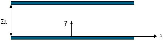
Figure 1.
Channel geometry and coordinate system.
Figure 1.
Channel geometry and coordinate system.

In this paper ( denote the streamwise, wall-normal, and spanwise averaged-in-time velocity components at a point, ( the corresponding velocity fluctuations, and the time-averaged pressure. The time-averaged flow is parallel, i.e., the mean velocity field is (, 0, 0), and the mean streamwise velocity component is a function of the distance from the lower wall.
Simplifying the Reynolds-averaged Navier–Stokes (RANS) equations for fully developed incompressible turbulent flow, one obtains the following:
We note that the Reynolds shear stress term in Equation (1) cannot be neglected and that the mean pressure at a cross-section x = const. is a function of due to Equation (2).
After some mathematical manipulations of Equations (1) and (2) one finds the following:
where is the friction velocity, is the mean shear stress at the wall, the kinematic viscosity, and the fluid density. The wall pressure gradient in the streamwise direction is related to the mean shear stress at the wall, , by the relation:
Equation (3), expressed in terms of the inner-law variables , , is put in the dimensionless form:
where is the friction Reynolds number formed using the channel half height as characteristic length and the friction velocity as characteristic velocity. The term corresponds to the normalized Reynolds shear stress .
3. Analysis of DNS Datasets
In this work we consider DNS data published by Lee and Moser [1], Bernardini, Pirozzoli and Orlandi [2], Lozano-Durán and Jimenez [3], Yamamoto and Tsuji [4], and Hoyas, Oberlack et al. [5] and discuss their salient features. The specific DNS datasets analyzed in the present work are listed in Table 1 together with the friction Reynolds number corresponding to each dataset.

Table 1.
Datasets analyzed in the present study. .
3.1. Mean Velocity Profiles (MVPs) and Integration-Based Quantities
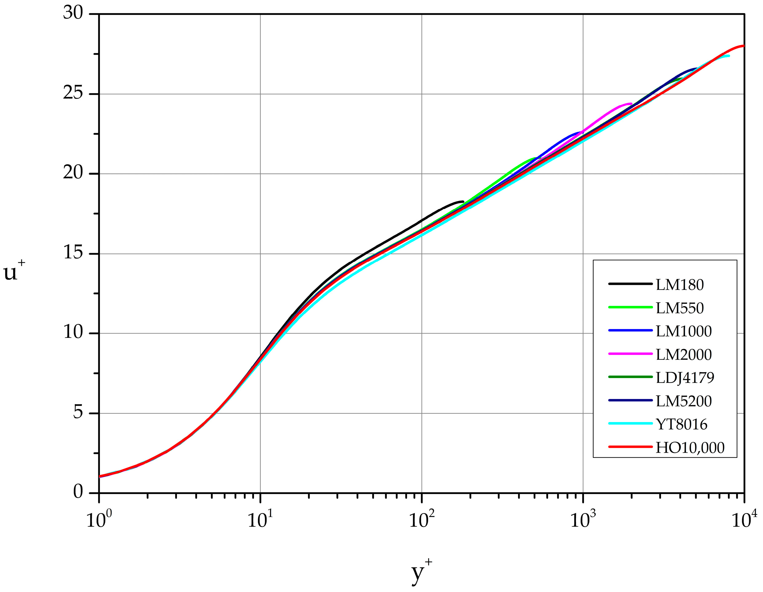
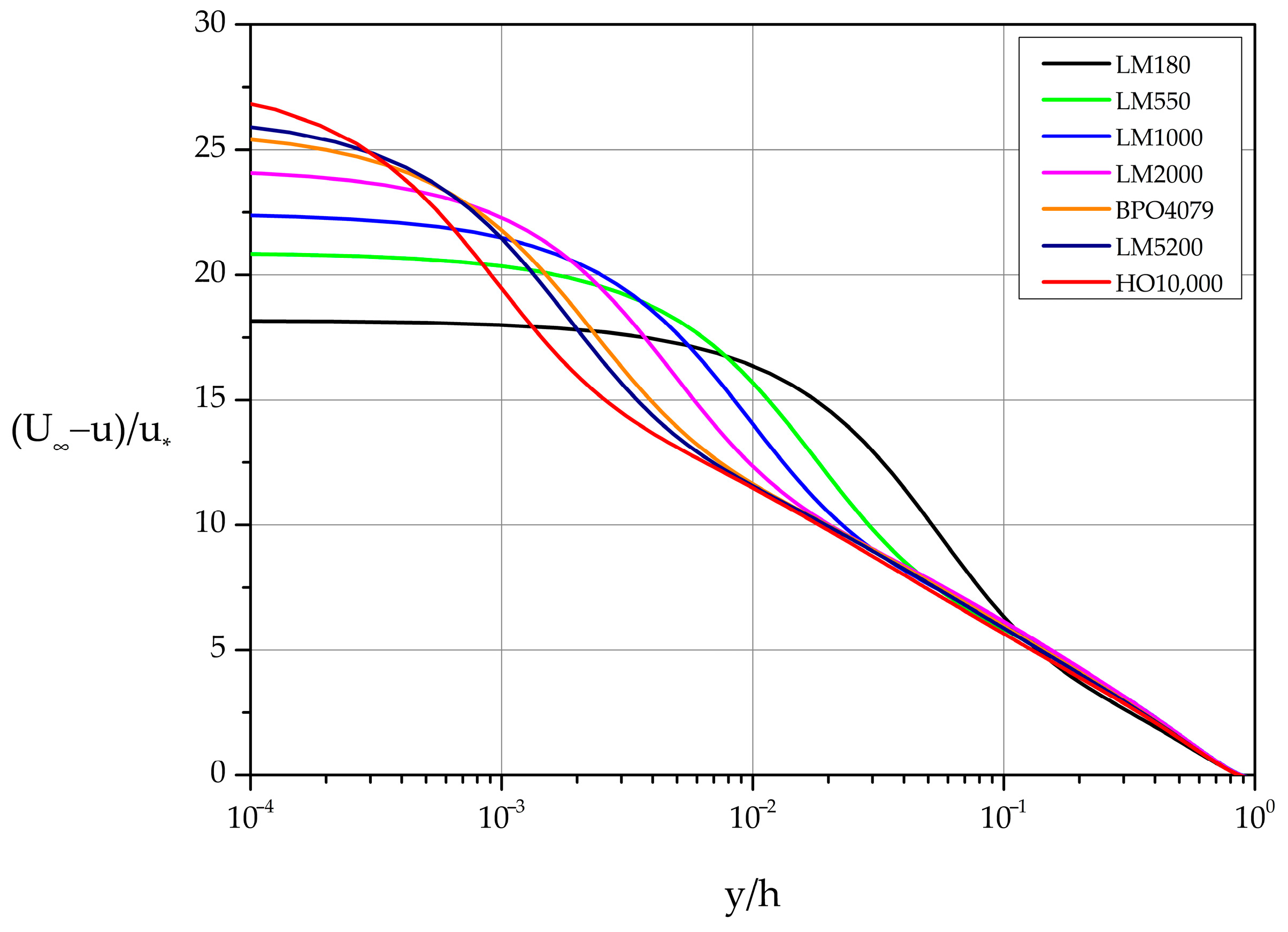
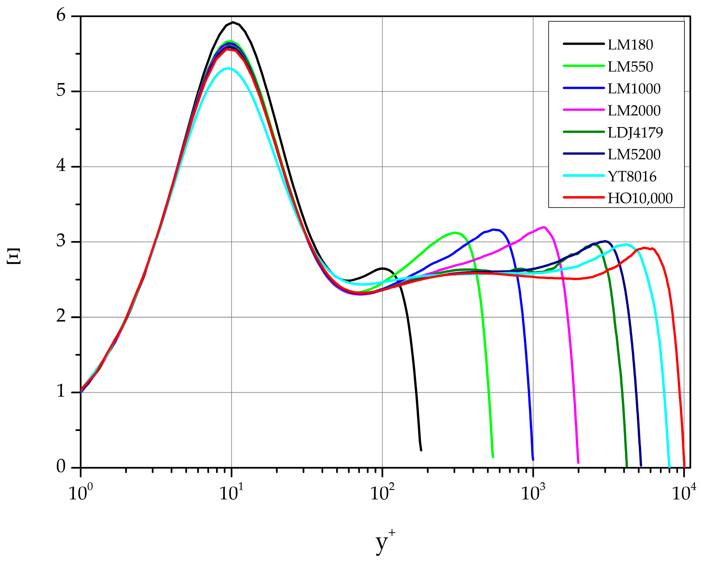
Figure 2 shows the velocity profiles in law of the wall variables (, ) while Figure 3 presents the same data in the standard velocity defect form. The Reynolds number independence of near the wall is captured with perfect accuracy for all Reynolds numbers listed in Table 1. On the other hand, the Reynolds number independence far from the wall in velocity defect variables shows small deviations (especially for the smaller Reynolds number cases) from the theoretical collapse to a single curve demanded by similarity considerations.
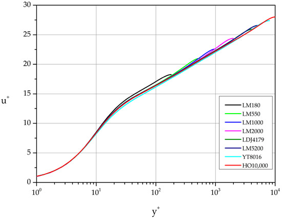
Figure 2.
Mean velocity profiles expressed in law of the wall variables.
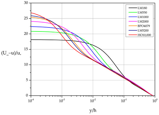
Figure 3.
Mean velocity profiles expressed in velocity defect law variables.
Based on the DNS mean velocity profiles, one can calculate the cross-sectional average velocity, , and the dimensionless ratio . As it is customary, in canonical wall-bounded flows (straight pipes and channels of constant cross-section) we calculate the resistance law in the form of the friction factor , or equivalently the skin friction coefficient, . In the case of channel flow, the Darcy–Weisbach equation [8] takes the following form:
where is the hydraulic diameter of the channel cross-section and denotes the bulk (cross-sectional average) velocity. For the 2D channel shown in Figure 1 (cross-section of “infinite” aspect ratio), the hydraulic diameter and consequently considering Equation (4):
Alternatively, we can work with the skin friction coefficient defined as follows:
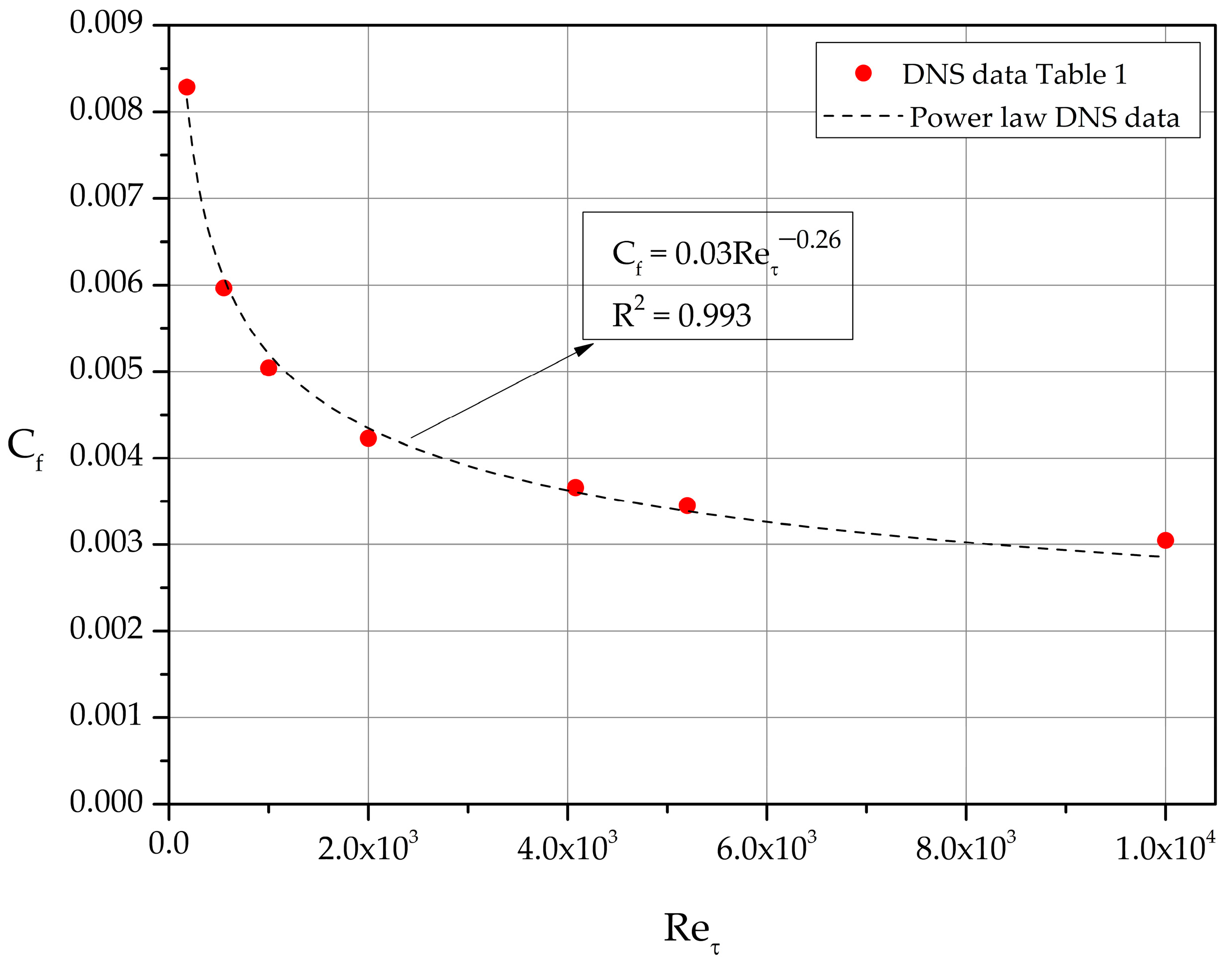
The calculated values of for each dataset of Table 1 are shown as filled circles in Figure 4. Least-squares fit reveals the power-law relation:
valid in the range 180 10,000.
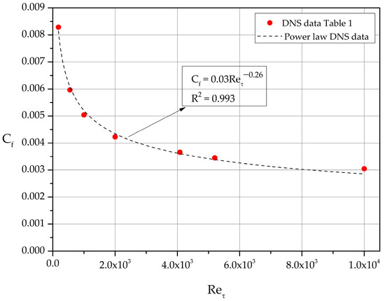
Figure 4.
Skin friction coefficient as function of .
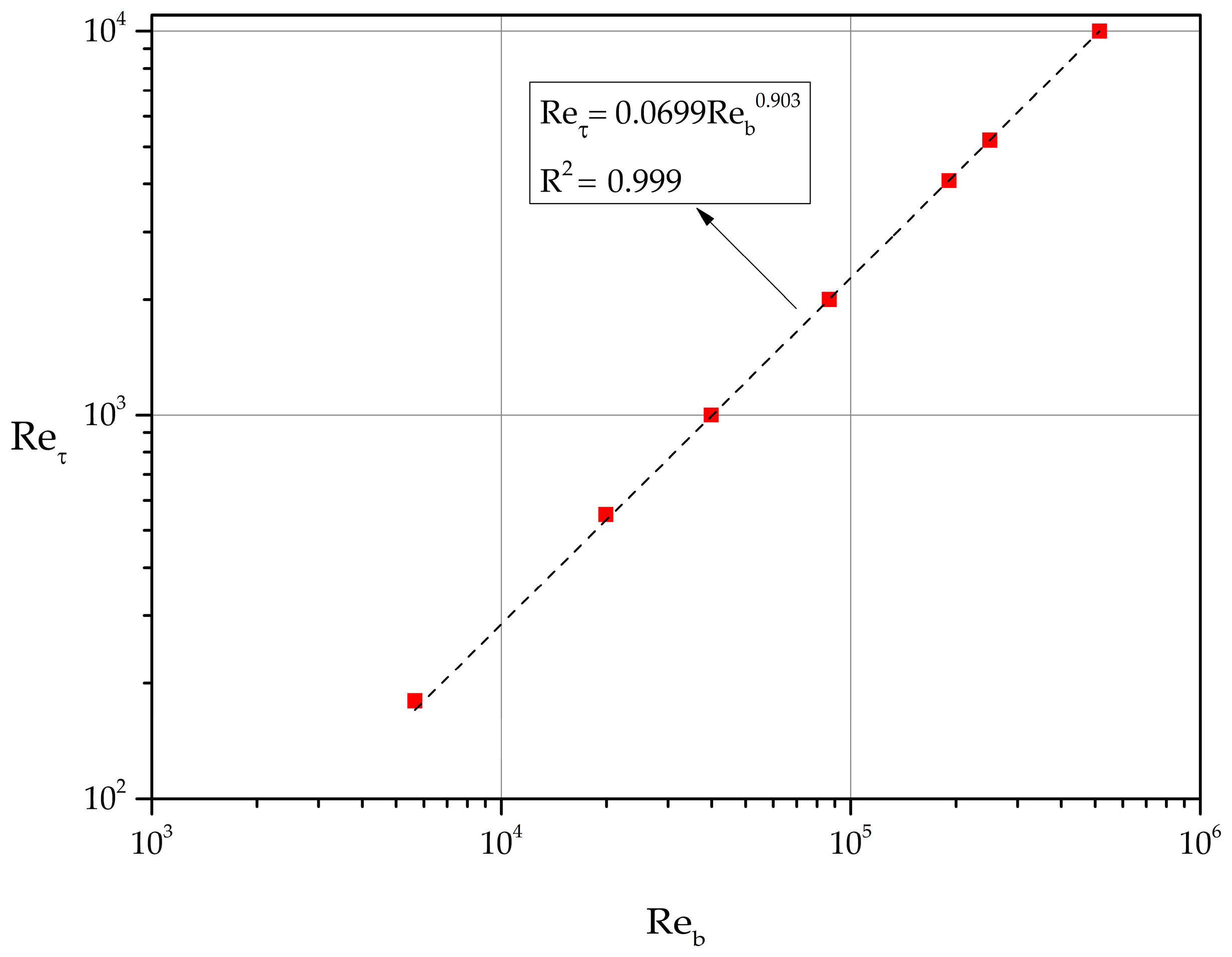
The relation between the bulk Reynolds number as and is found to be with excellent accuracy (see Figure 5). It follows that
based on least-squares fit.
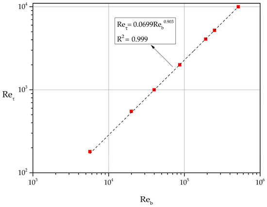
Figure 5.
Relation between and .
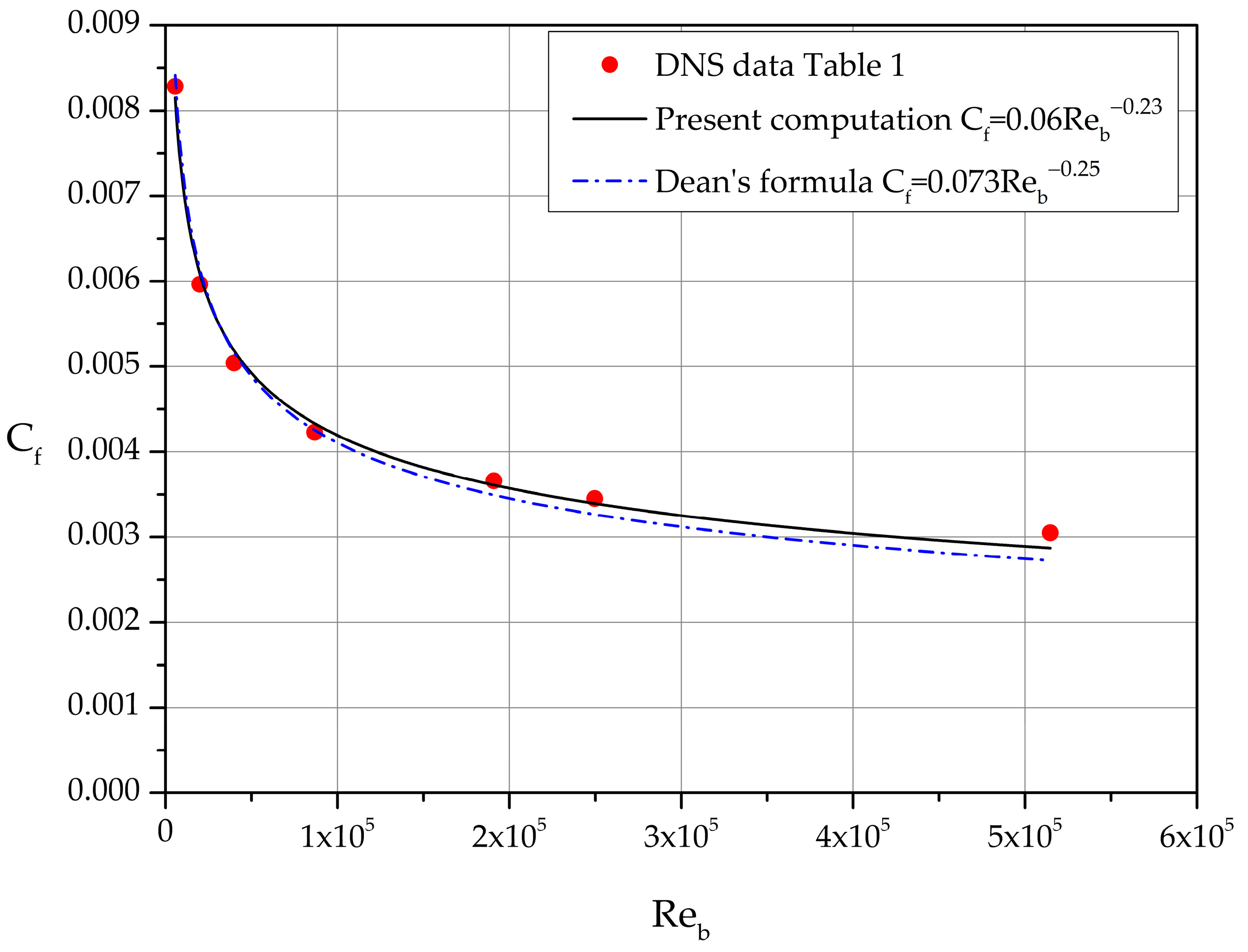
The skin friction coefficient expressed as function of differs slightly from Dean’s formula [9]:
Dean based his formula on selected experimental measurements of high Reynolds number flows in channels with cross-section aspect ratio greater than 1:12 [9,10]. The comparison is shown in graphical form in Figure 6.
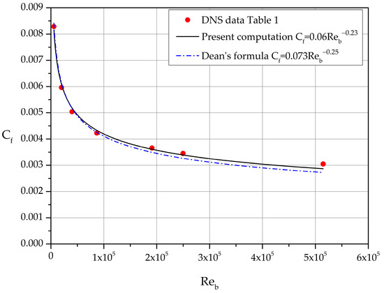
Figure 6.
Comparison of DNS-based Equation (10) with Dean’s formula, Equation (11).
In a recently published work, Nucci and Absi [11] analyzed DNS data for low Reynolds numbers in the range 110 2000. Their computed values for differ slightly from the skin friction Equation (9).
Next, we consider the lower half of the channel flow as a boundary layer of thickness δ = h and introduce the skin friction coefficient where U . Introducing the friction velocity, , in the local skin friction coefficient definition we obtain the following:
A least-squares fit of the values, computed based on the DNS datasets of Table 1, is shown in Figure 7.
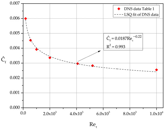
Figure 7.
Dependence of the alternate skin friction coefficient on .
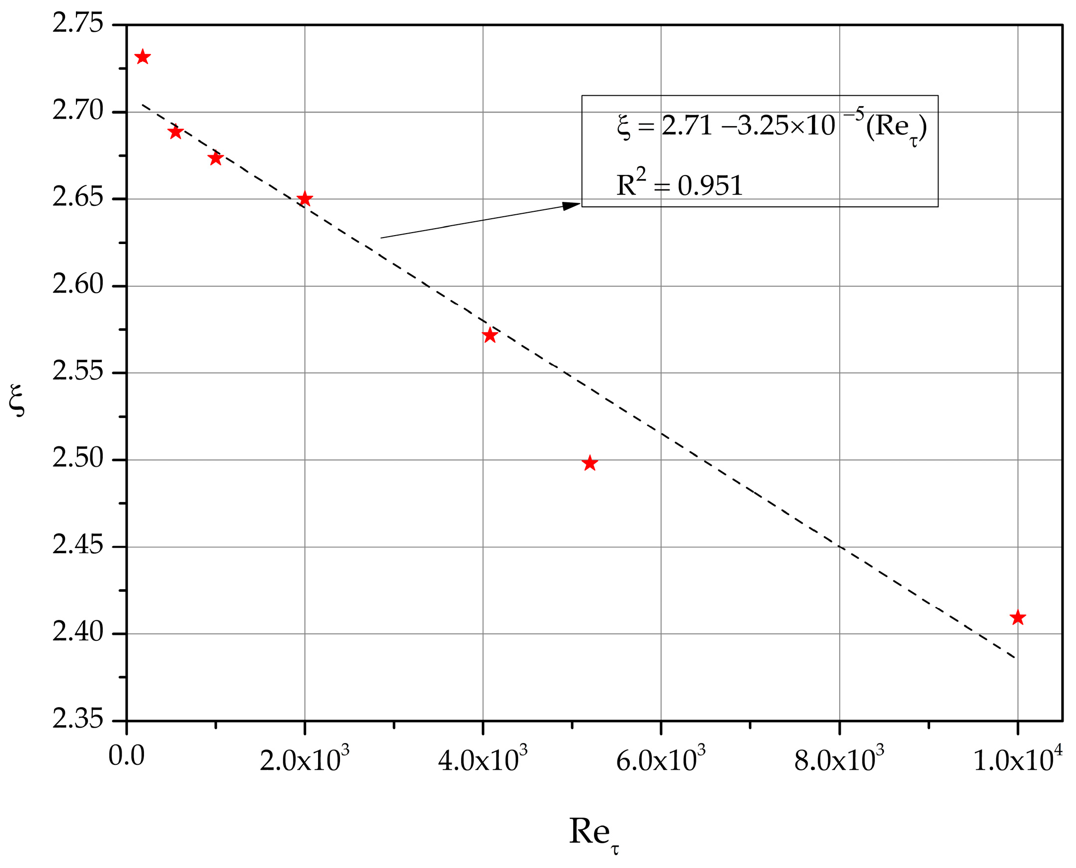
It is worth commenting on the mean velocity profile in the central region of the channel flow. We define the following:
and list the computed values in Table 2.
Table 2.
Reynolds number dependence of
A least-squares fit of the values , calculated for the DNS datasets of Table 1, is shown in Figure 8.
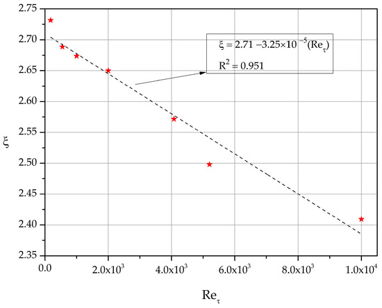
Figure 8.
Least-squares fit of ξ versus .
The linear relation gives a fair approximation of the function in the range of the values considered in this work. It clearly shows the correct trend since in the limit of infinite Reynolds number ξ should tend to zero.
3.2. Diagnostic Functions Ξ and Γ for the MVP
A great deal of research has been conducted and lively discussions have arisen in the scientific literature as to whether a logarithmic or a power function describes better the overlap region of the MVP. To decipher where these approximations fit the data better, two diagnostic functions may be used.
The first function, defined as Ξ , serves to detect intervals where is a logarithmic function of . It is easy to prove that when Ξ attains a constant value, exhibits a logarithmic behavior of the following form:
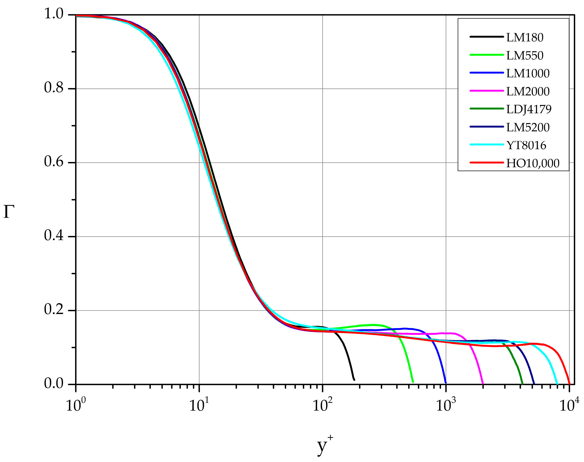
The second diagnostic function, defined as Γ , is useful in detecting intervals where is approximated well by a power function of the following form:
In the interval where Γ const., is approximated by a function of the form (15) with λ = Γ.
Both diagnostic functions require the computation of the derivative . Since numerical differentiation acts as an error amplifier, analyzing the DNS data in terms of the two diagnostic functions helps us to indicate the interval of the appropriate approximation with greater confidence and accuracy.
To avoid misunderstandings in the remainder of this section it should be stressed that the logarithmic law, Equation (14), is theoretically valid only asymptotically for . The logarithmic law has been derived based on various sets of assumptions. The well-known Millikan’s [12] argument is based on the notion that, in the intermediate region (layer), both the wall law and the velocity defect laws should be valid. In the limit of infinite Reynolds number this leads to the existence of a logarithmic layer in the overlap (inertial) region. Landau’s [13] treatment of the infinite flat plate in terms of the notion of “logarithmic accuracy” also provides a firm ground for the existence of logarithmic behavior. There are two schools of thought with respect to the constant (κ is the von Kármán constant) in Equation (14). One insists that κ is a universal constant while the other maintains that the value of κ depends on the type (geometry) of the flow [14,15,16,17,18,19,20,21,22].
For finite Reynolds number turbulent flows, several researchers [23,24,25,26,27] have argued that a power law (with Reynolds number dependent coefficients) fits the experimental and DNS results better.
In this work the numerical evaluation of the derivative is performed using the following formula for unequally spaced data:
3.2.1. Diagnostic Function Ξ
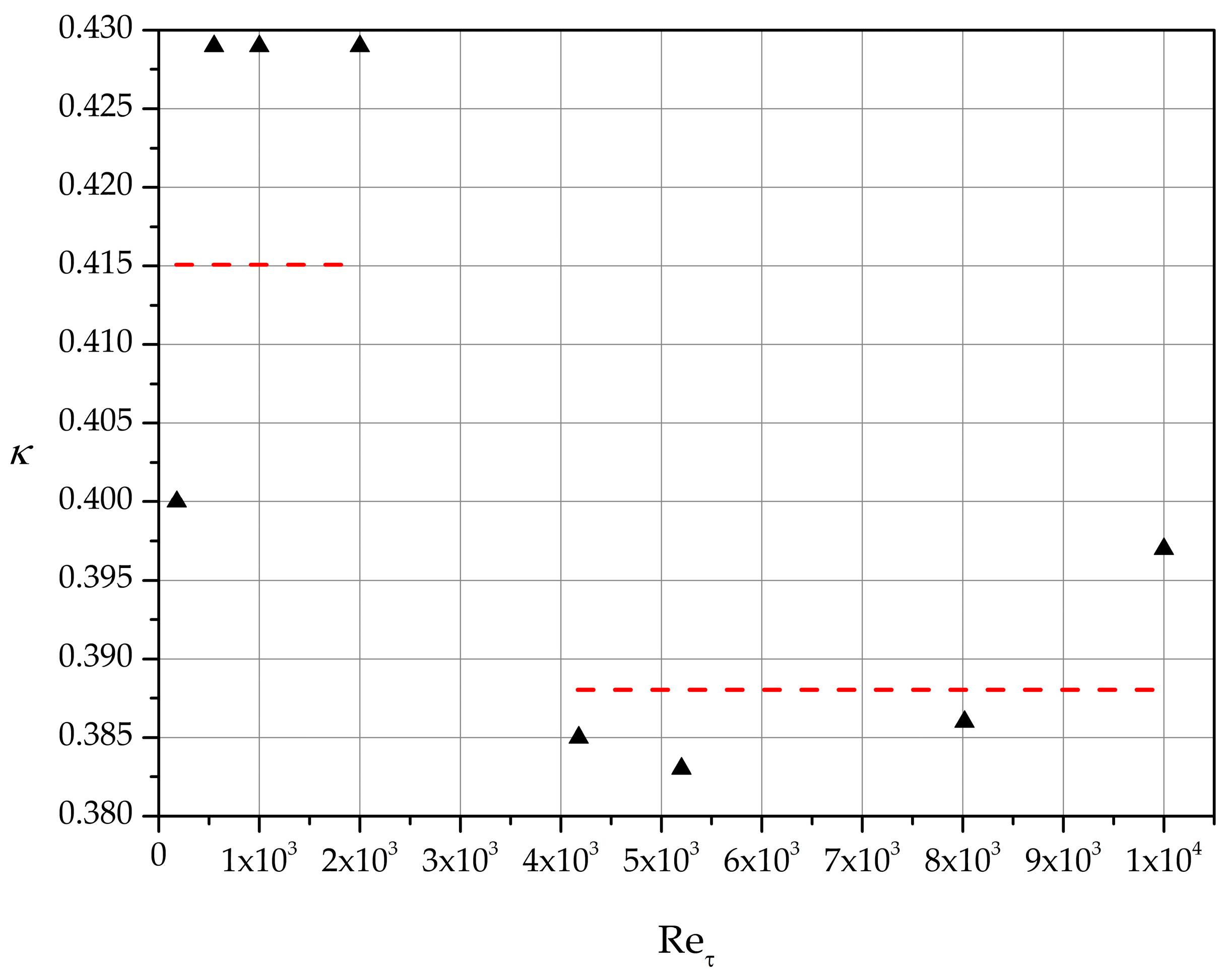
Figure 9 depicts the calculated curves for the cases listed in Table 1. As increases the intervals where Ξ is approximately constant become longer, which implies an increase of the log-law region. In Table 3 our estimates of κ are listed together with the intervals where Ξ const. .
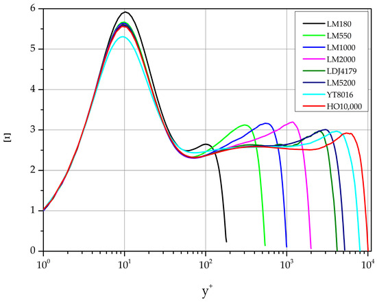
Figure 9.
Diagnostic function Ξ based on DNS datasets of Table 1.
Table 3.
Estimation of the von Kármán constant.
For 180 our estimate of the von Kármán constant is κ 0.40 while for 550, 1000, 2000 κ 0.429. For higher values of friction Reynolds number in the range [4000–10,000], a good representative value for κ is 0.388. Finally, a good overall approximation of κ in the range [180–10,000] is found to be 0.405 (see Figure 10). These values are in general agreement with some of the most recent von Kármán constant estimates reported in the literature. For further details the reader is referred to references [28,29,30].
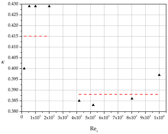
Figure 10.
Von Kármán constant estimates and average representative values for low and high friction Reynolds numbers.
3.2.2. Diagnostic Function Γ
Figure 11 depicts the variation of Γ function for each dataset listed in Table 1. Analyzing the behavior of these curves we identify intervals [ where Γ attains a constant value. These intervals together with the implied values of the exponent λ in Equation (15) are listed in Table 4.
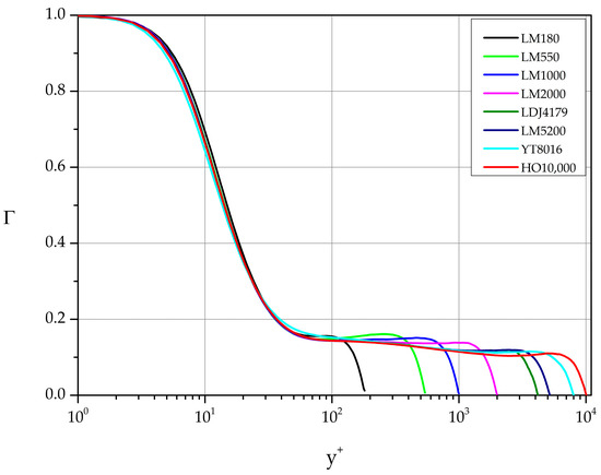
Figure 11.
Diagnostic function Γ based on the DNS datasets of Table 1.
Table 4.
Estimates of the λ exponent in the power-law Equation (15).
3.3. Second Order Statistics
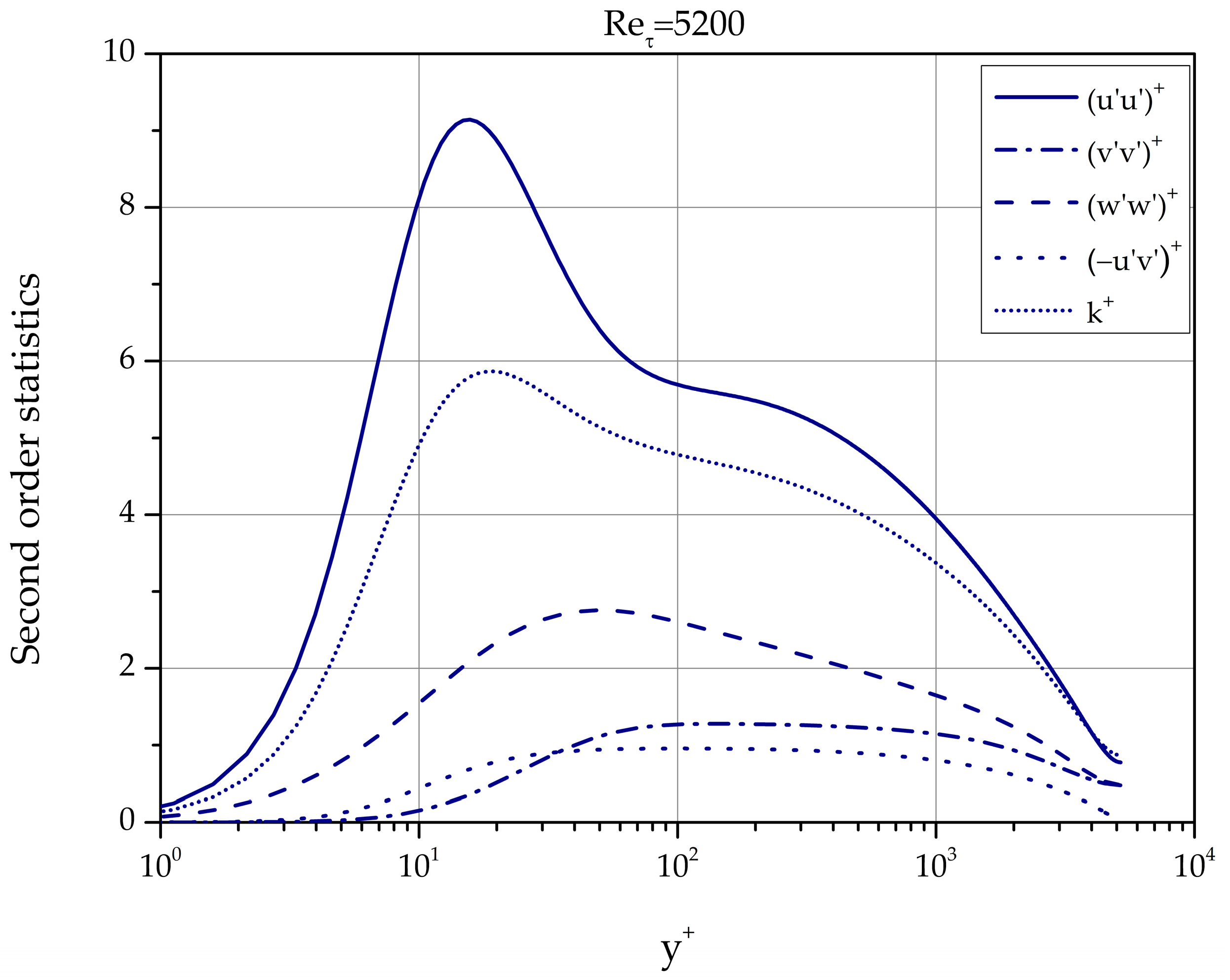
Typical profiles of the normal and shear Reynolds stresses as well as of the turbulence kinetic energy are shown in Figure 12 for 5200.
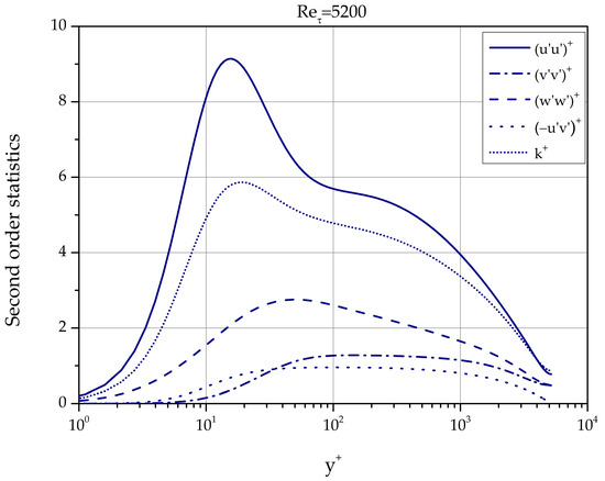
Figure 12.
Second order statistics of turbulence fluctuations for = 5200. All data are normalized with . Case: LM5200.
In the remainder of Section 3 we explore the Reynolds number effects on second order statistics of turbulence fluctuations. A logarithmic region is expected in the streamwise and spanwise normal Reynolds stresses at sufficiently high Reynolds number [31,32,33,34,35,36]. We also discuss below the Reynolds number dependence (or independence) of the Reynolds stresses and turbulence kinetic energy [37,38,39].
3.3.1.
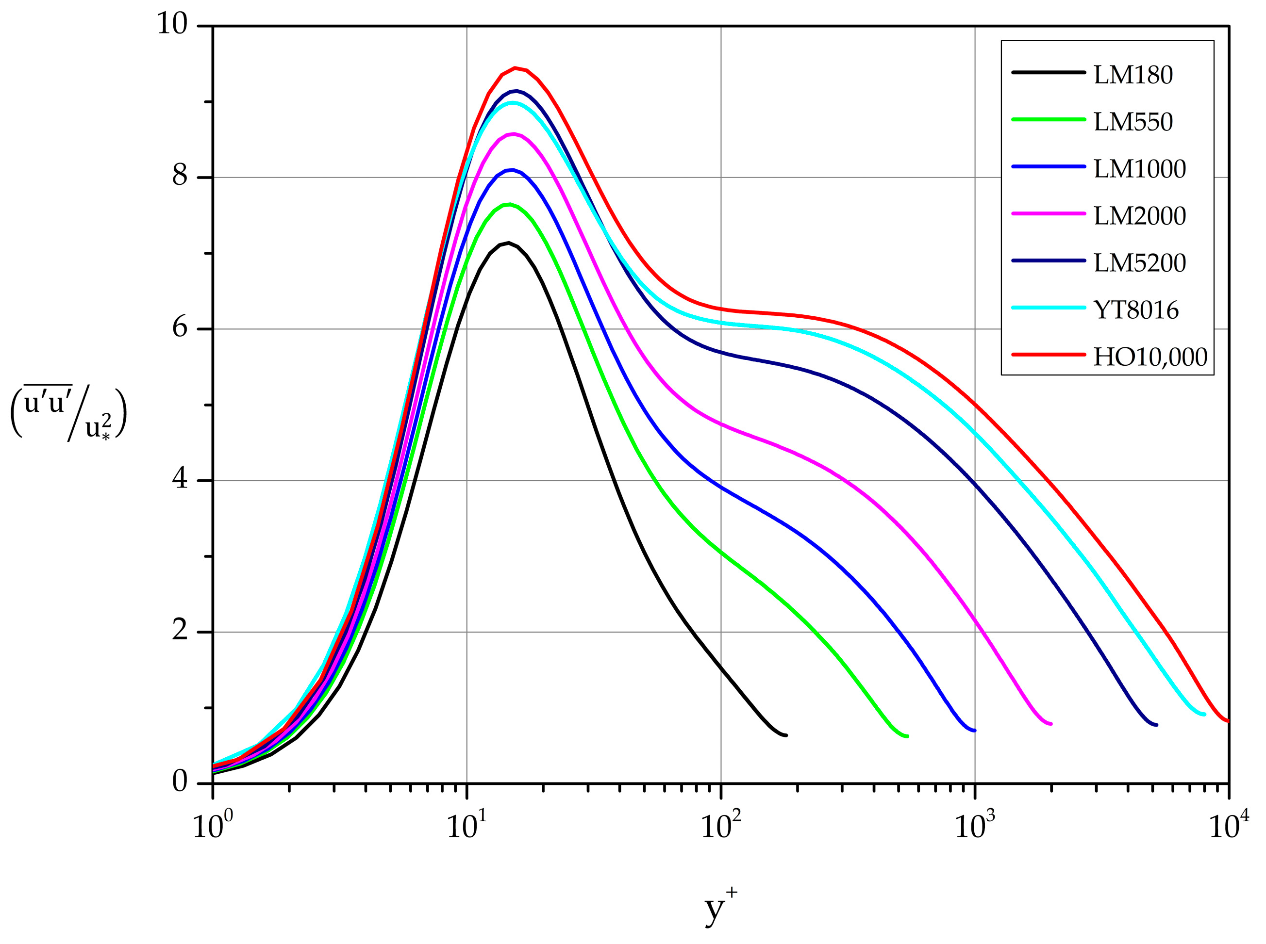
The normalized variance profiles of the streamwise fluctuations are shown in Figure 13. A clear maximum characterizes each curve. Least-squares fit gives the following expression for the near wall maxima of the normalized variance profiles of streamwise fluctuations:
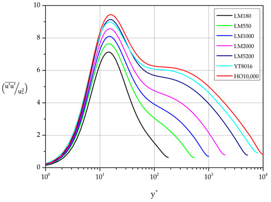
Figure 13.
Streamwise fluctuations. Normalized variance profiles.
Turning now to the search for logarithmic behavior in , we search for a relation of the following form:
where is the Townsend–Perry constant and an additive parameter that depends on Reynolds number [34]. The term “sufficiently high Reynolds number” in this case means 7000 [4]. Calculating and plotting the indicator function
we have identified regions of logarithmic variation in the cases YT8016 and HO10,000 (see Figure 13 and Table 5).
Table 5.
Estimates of Townsend–Perry parameters.
The values on the top two lines compare quite well with the values given in the literature for and [4,31,32,33]. However, we have opted to list additional intervals at larger distances from the wall where behavior of the form (18) can be identified.
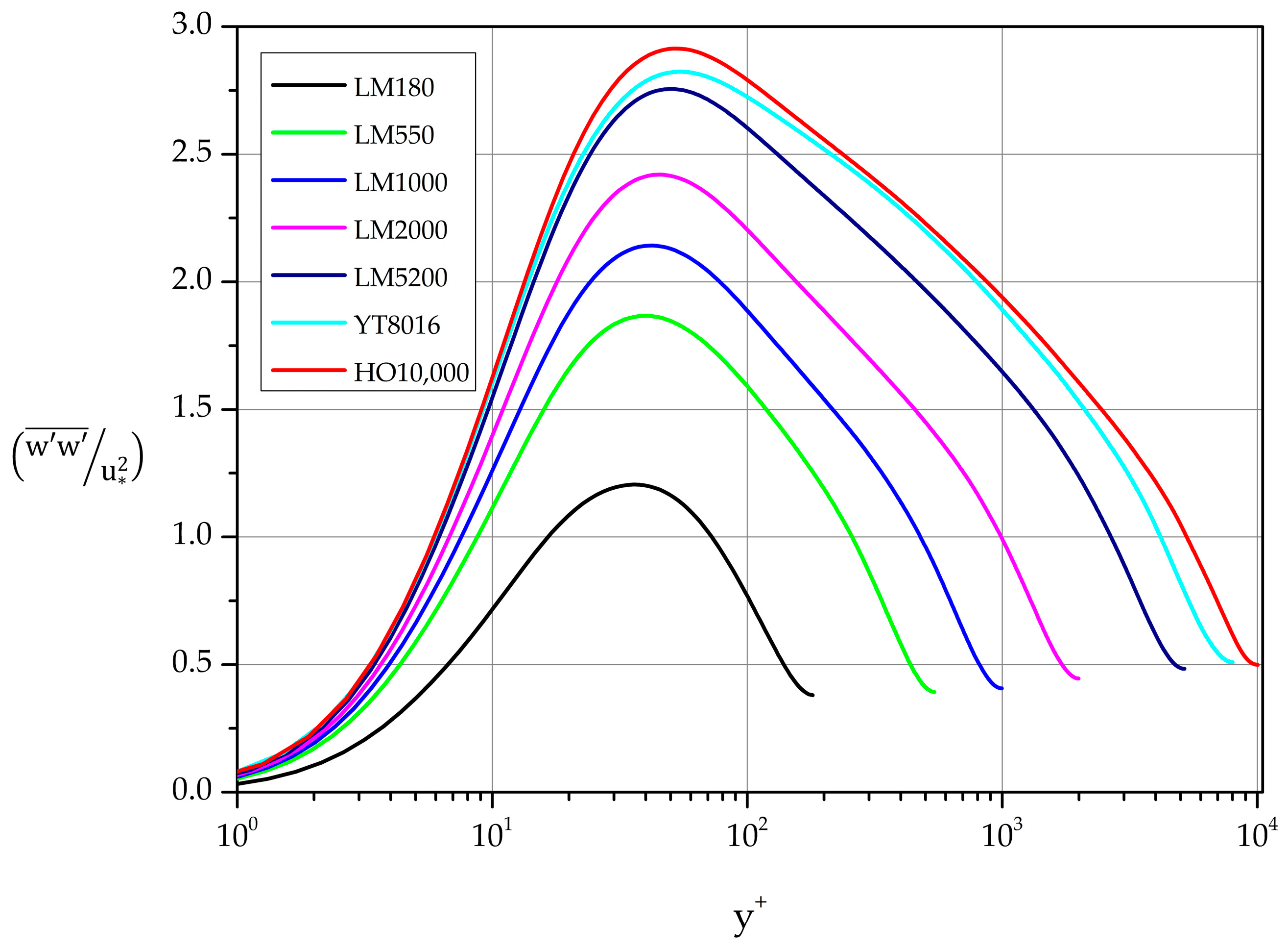
3.3.2.
The variance profiles of the spanwise fluctuations are shown in Figure 14. A near wall maximum characterizes each profile. Least-squares fit gives the following dependence on :
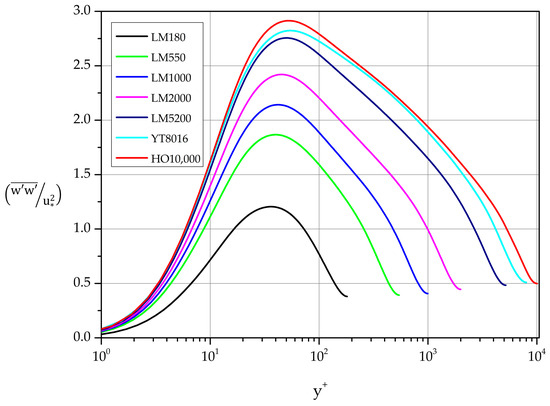
Figure 14.
Normalized spanwise fluctuations. Variance profiles.
Next, we search for regions of logarithmic behavior of the following form:
With the help of the appropriate indicator function we estimate the constant and the additive parameter as shown in Table 6.
Table 6.
. Estimates of Townsend–Perry parameters.
Obviously, some regions can be merged by relaxing the tolerance allowed on deviations from the requirement of constancy of the diagnostic function. We also note that in we observe logarithmic behavior for as low as 2000. As in Table 5, we have opted to list additional intervals where behavior of the form (21) can be identified.
3.3.3.
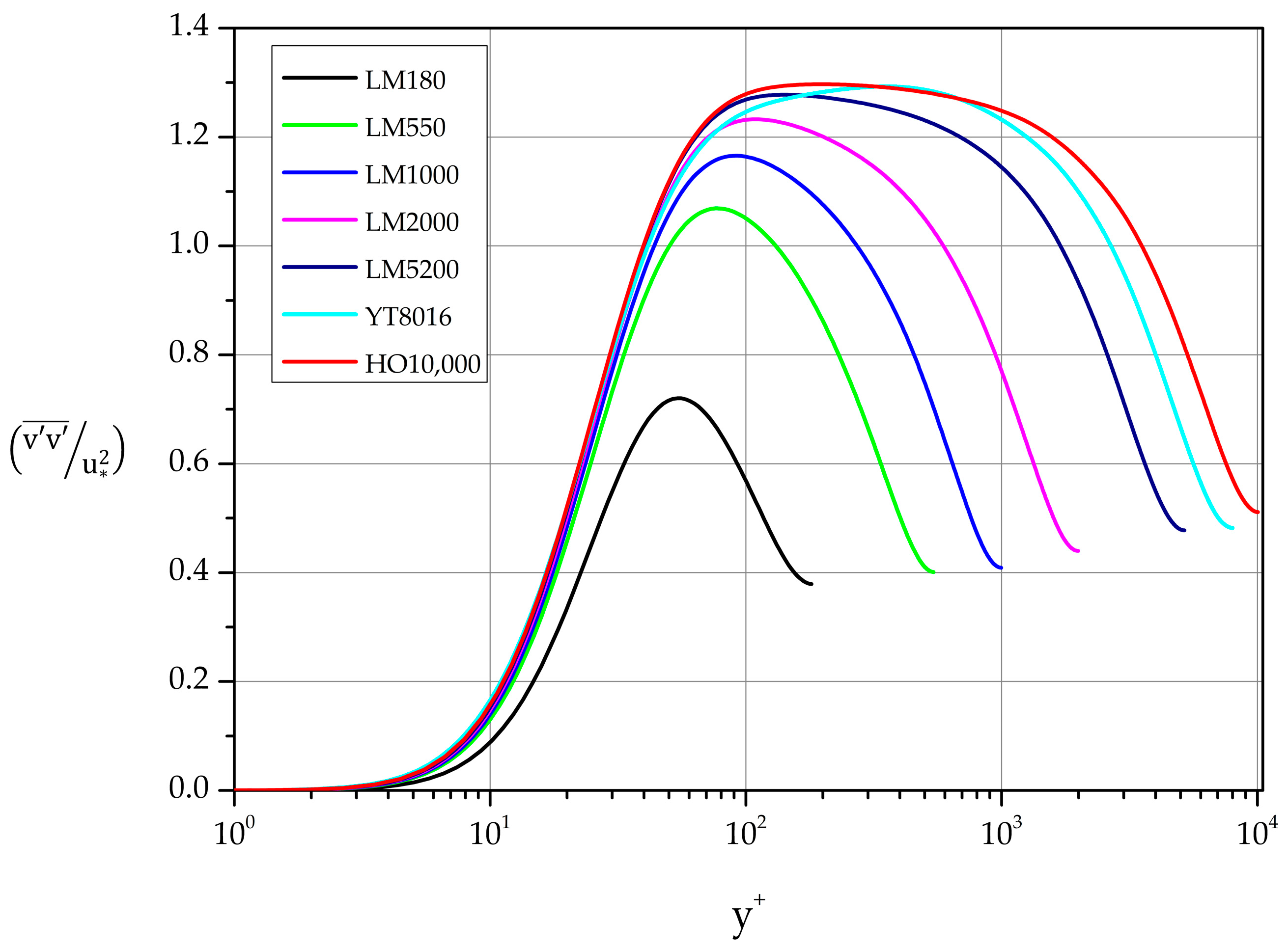
The variance profiles of wall-normal fluctuations (Figure 15) exhibit a different behavior for high Reynolds number:
in the interval 150 550 for 8016 and 10,000. In particularly, case YT8016 displays a constant 1.29 in the region 250 550 while in case HO10,000 1.30 in the interval 150 450.
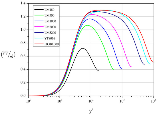
Figure 15.
Normalized wall-normal fluctuations. Variance profiles.
In the lower Reynolds number cases a plateau is not formed. Instead, clear maxima are formed for 180 5200. A least-squares fit approximates the dependence on , as follows:
in the range 550 10,000.
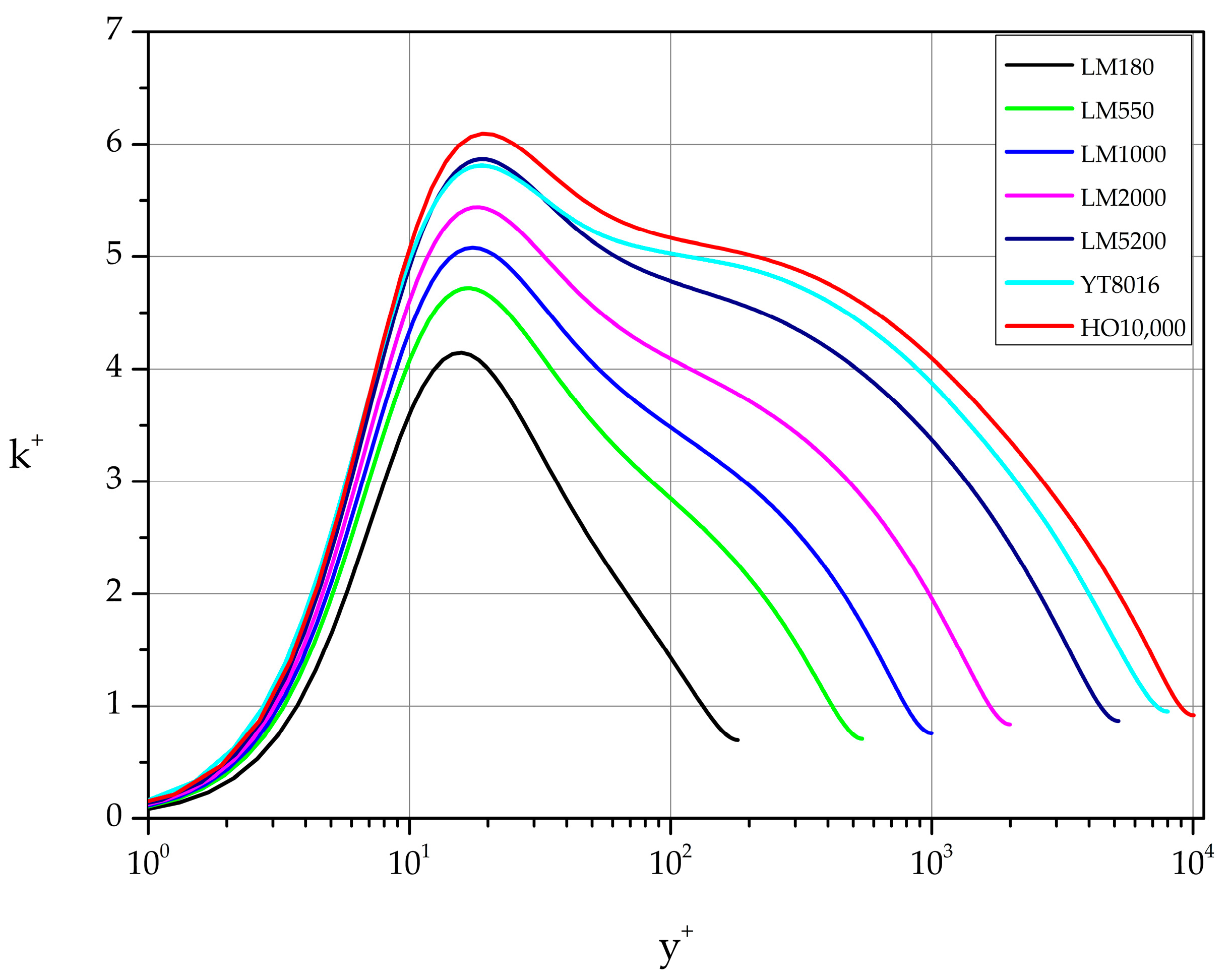
3.3.4. Turbulence Kinetic Energy, k
Each nondimensional turbulence kinetic energy profile is characterized by a maximum at approximately 18. The exact location of the maximum is weakly influenced by (see Table 7). The normalized value is strongly influenced by in the range of the Reynolds number values considered (see Figure 16 and Table 7).
Table 7.
Reynolds number effect on .
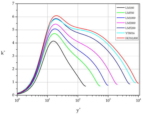
Figure 16.
Normalized turbulence kinetic energy profiles.
Least squares fit of the (, ) pairs of values gives the following relation:
and describes the function with very good approximation.
Turning to the question of existence or not of logarithmic behavior in the turbulence kinetic energy profiles of the following form:
we have identified the regions listed in Table 8.
Table 8.
Logarithmic behavior regions in .
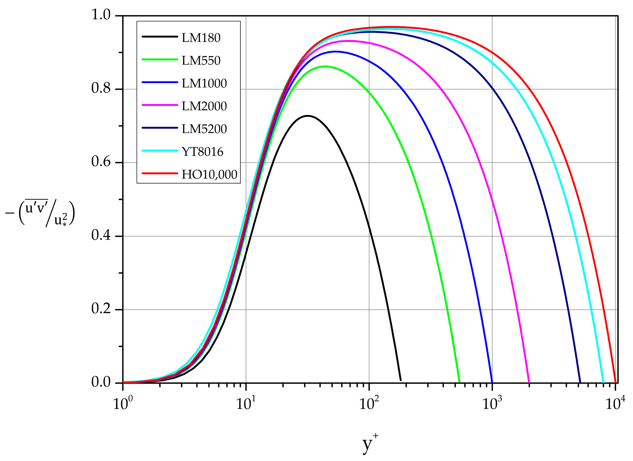
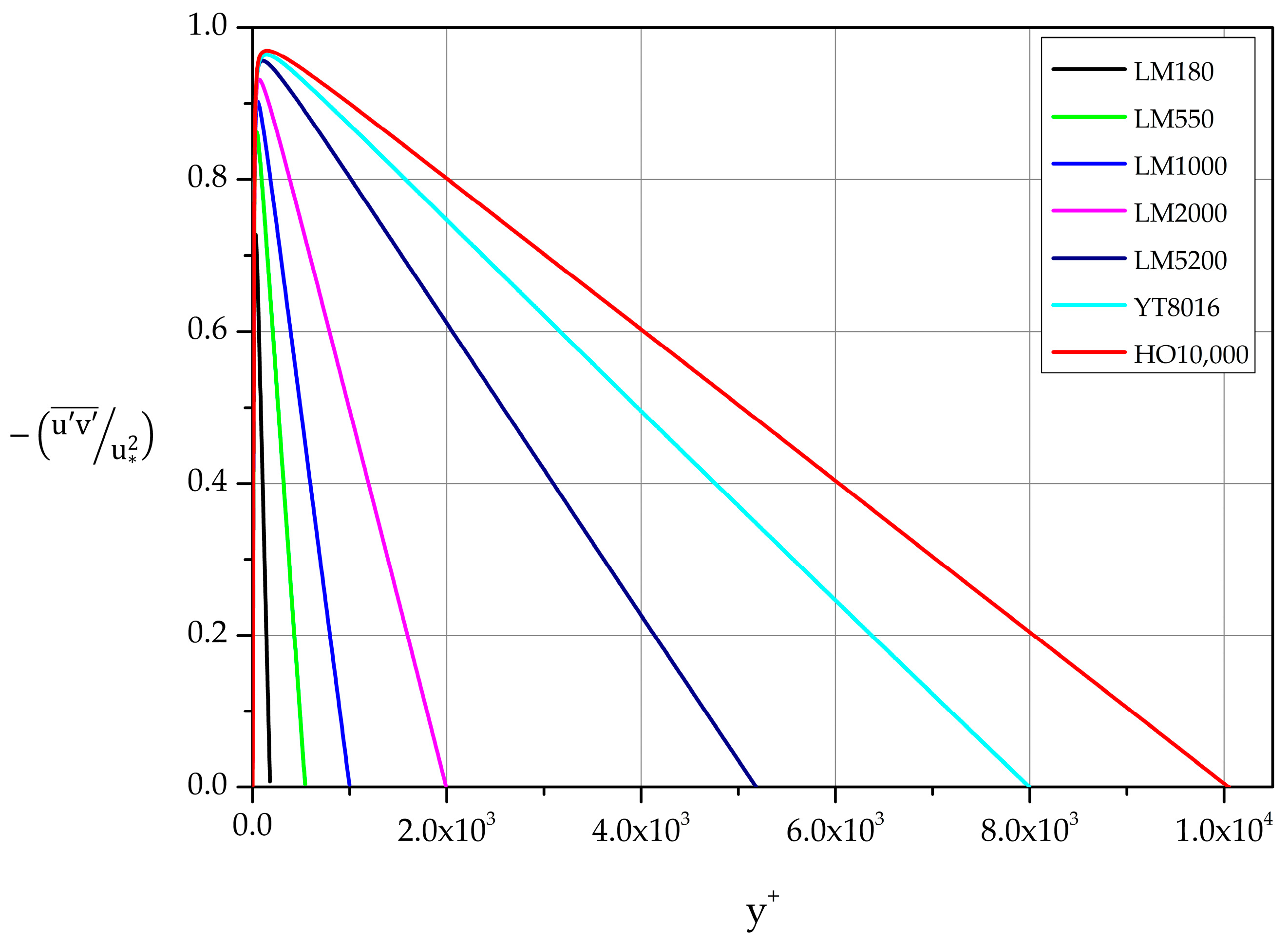
3.3.5. Reynolds Shear Stress
Profiles of the normalized covariance of streamwise and wall-normal fluctuations are shown in Figure 17 and Figure 18. They are strongly influenced by Reynolds number. For equal to 8016 and 10,000 a clear plateau is formed. Specifically,
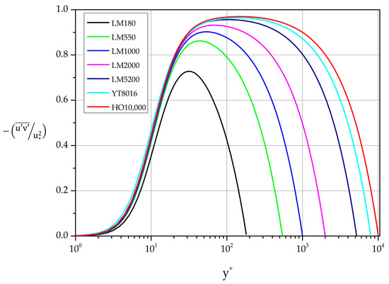
Figure 17.
Normalized covariance profiles of streamwise and wall-normal fluctuations in law of the wall variables.
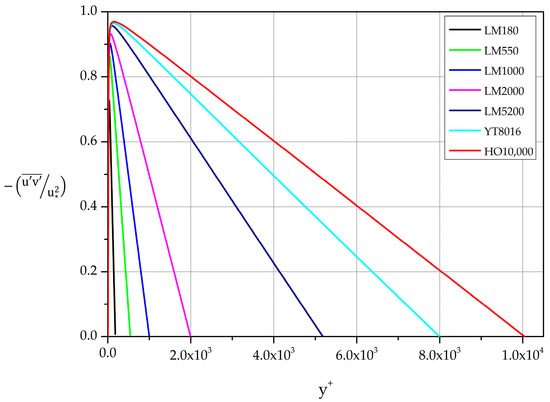
Figure 18.
Normalized covariance profiles of the streamwise and wall-normal fluctuations in law of the wall variables.
at 8016: 0.963 in the interval [100–200]
at 10,000: 0.969 in the interval [100–250]
The maxima of the curves in the range 550 10,000 follow the relation:
obtained by least-squares fit, while the location of the varies with according to the following relation:
for the same range of .
For large values of the derivative of the mean velocity is small compared to the Reynolds stress term in Equation (5). Consequently, we expect
i.e., the Reynolds shear stress varies linearly with distance from the wall in the region further than the layer closest to the wall [40]. This behavior is captured very accurately by the DNS data, as shown in Figure 18.
4. The AL84 Model
In this section the most important aspects of the AL84 model are outlined. The reader is referred to [6] for detailed description of the model construction and to reference [7] for a discussion on the accuracy of the AL84 model predictions for ZPG-TBL flows over a flat plate.
In the AL84 model the nondimensionalized mean velocity profile (MVP) is approximated by superposing two functions and , i.e.,
where
κ is the von Kármán constant and Π Coles’ [41] parameter.
Considering the channel cross-section as a whole, the flow rate per unit width of the channel is given by or, in terms of inner law variables, where . This integral is calculated as the sum of two terms, i.e., where
In the case of fully developed channel flow the boundary layer thickness is equal to the half-channel “height” and in wall-law variables . Analytical evaluation of the two integrals leads to the following expressions:
and
The average velocity at a channel cross-section is then given as and taking again into account the symmetry of the channel flow, the following is true:
In turn, the Darcy–Weisbach friction factor defined as can be calculated analytically based on Equation (35). The same information can be expressed in terms of the skin-friction coefficient .
We note that for pressure-driven channel flow, Equation (5) allows us to evaluate the Reynolds shear stress based on the AL84 model by inserting the derivative of the mean velocity with respect to (evaluated analytically based on Equations (30) and (31)) into Equation (5). This topic is discussed further in Section 4.3.
The authors believe that the model can be extended to compressible turbulent flows with minor but appropriate modifications using Favre averaging [42,43,44].
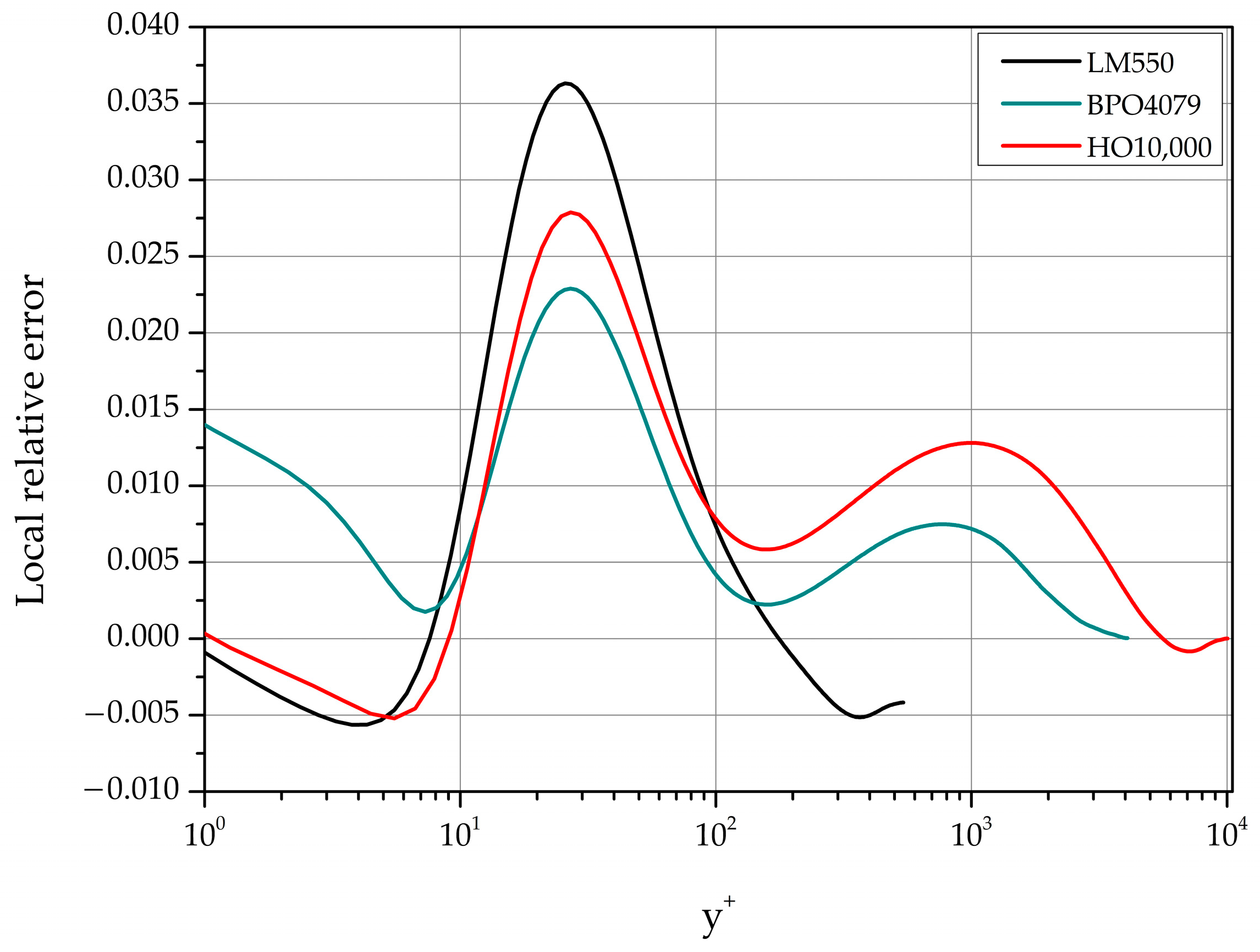
4.1. Global Absolute Error and Local Relative Error in AL84 Predictions
As explained in Reference [6], the values κ = 0.41 and the additive constant in the MVP logarithmic law = 5.0 (see Equation (14)) are incorporated in Equations (30) and (31) while the third parameter in AL84, Π, is free to vary with Reynolds number. Estimates of Π obtained from the DNS datasets analyzed are listed in Table 9.
Table 9.
Estimates of Coles’ parameter Π for channel flow.
The AL84 model performance is evaluated with these parameter values. The error at a distance from the lower channel wall is defined as e [g( Π)].
Representative local relative error profiles are shown in Figure 19 for three cases (low, moderate, and high) 550, 4079 and 10,000.
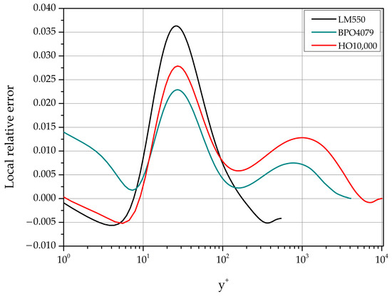
Figure 19.
Profiles of relative error in computed with AL84.
The maximum local relative error is located approximately at as shown in Table 10. In the range 2000 10,000 it is less than 3‰.
Table 10.
Maximum local relative error in AL84-based
The global statistics of the absolute error in the MVP approximation are summarized in Table 11.
Table 11.
Statistics of absolute error in the lower half of the channel 0 .
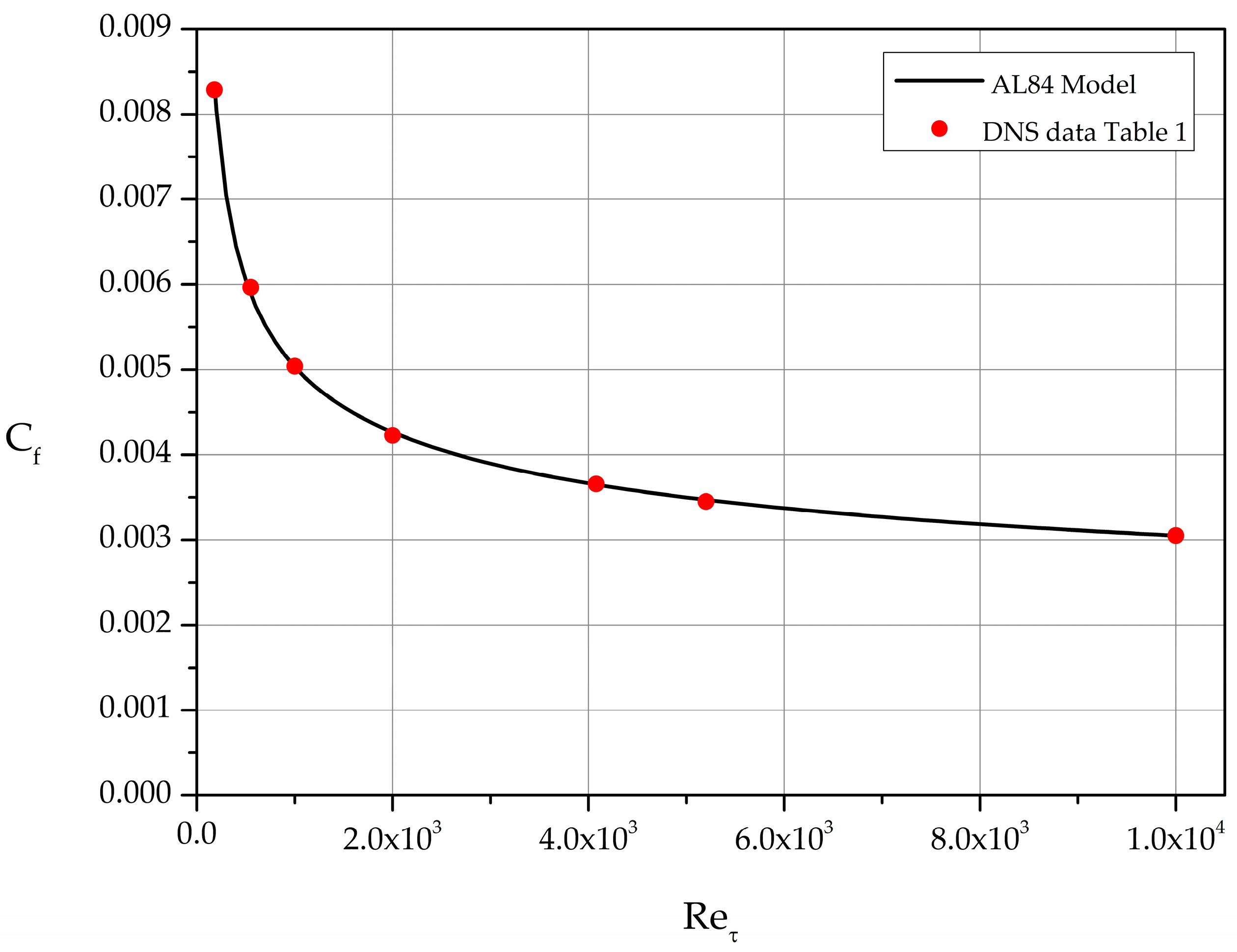
4.2. Cf Based on AL84
Comparing AL84-based results with those based solely on DNS we find that the agreement is excellent. The analytically computed curve passes exactly through the filled circles representing the values calculated directly from the datasets of Table 1 (see Figure 20).
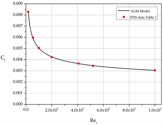
Figure 20.
Skin friction coefficient Cf. Comparison of AL84 model predictions with Cf computed for the DNS datasets of Table 1.
4.3. Reynolds Shear Stress ()
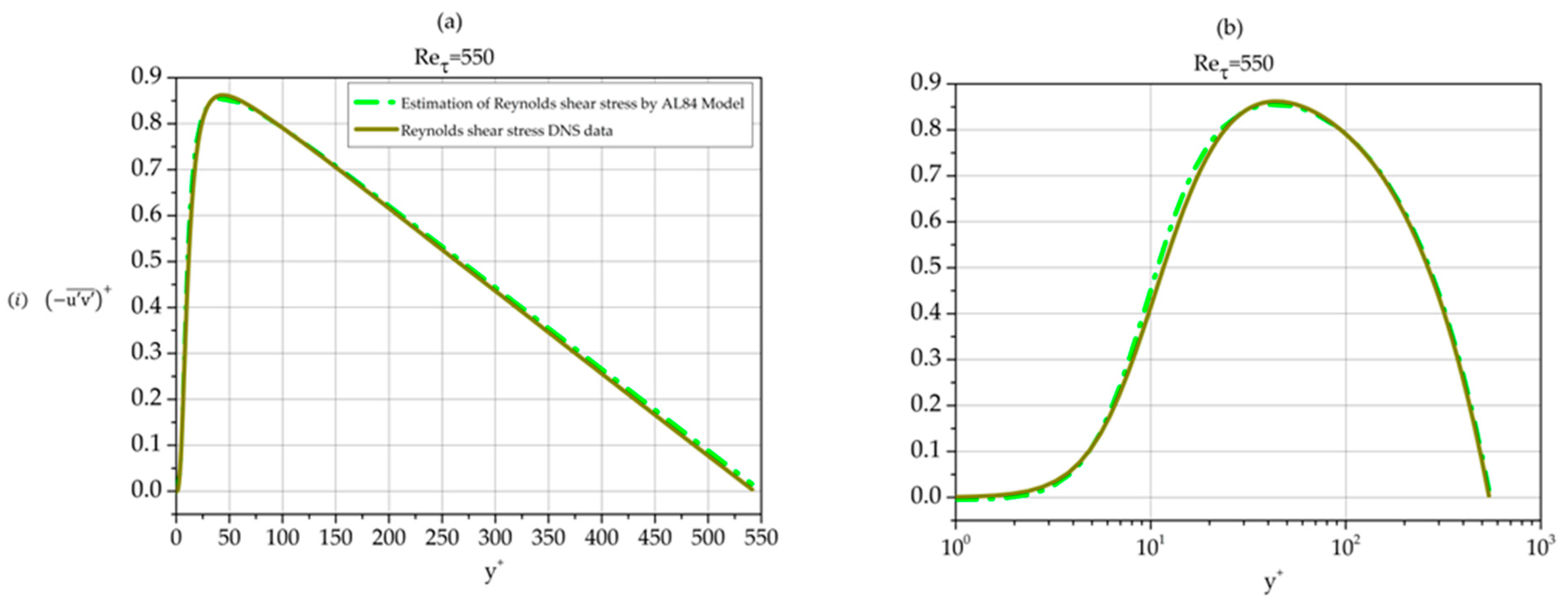
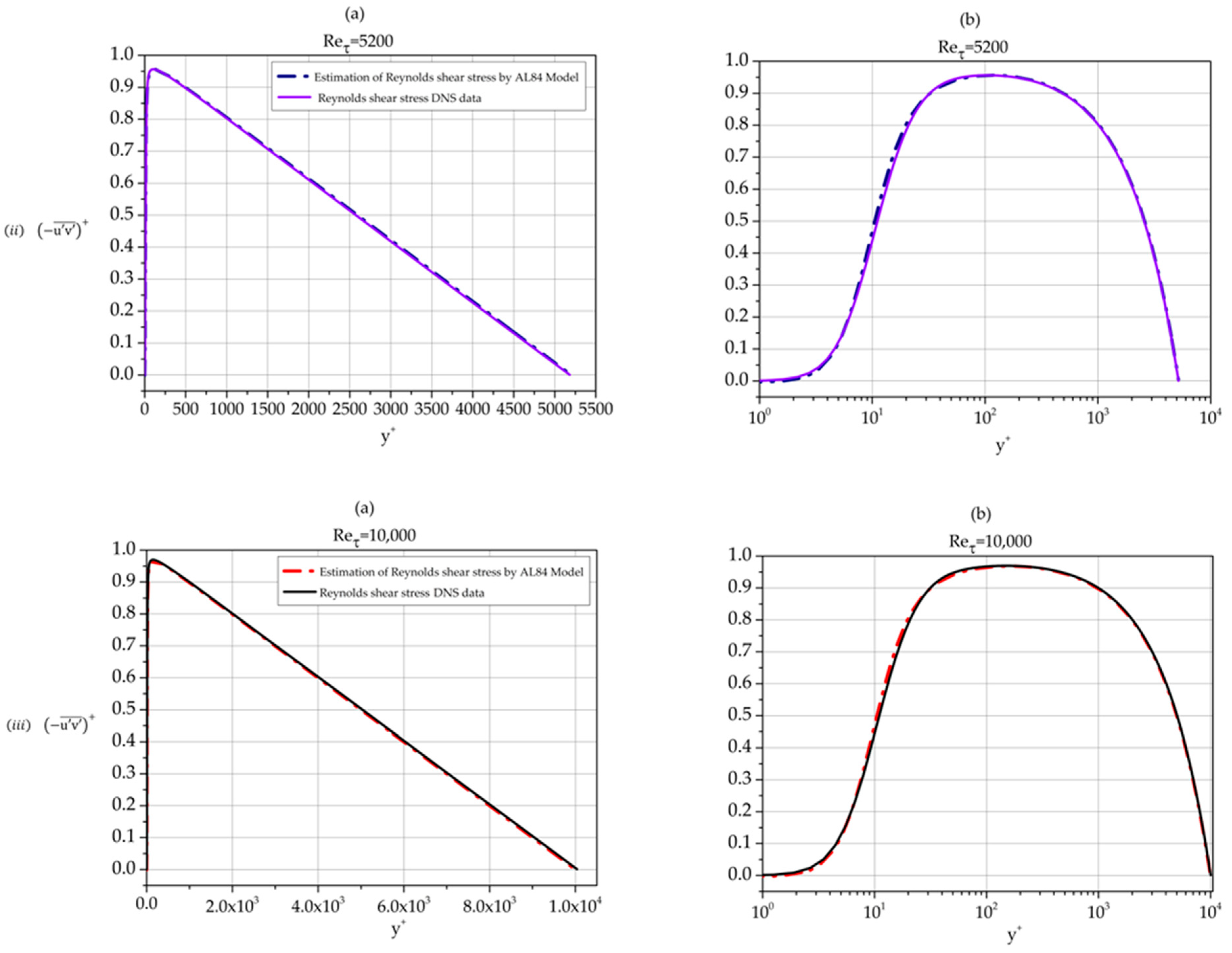
Using Equation (5), the covariance of fluctuations and as function of the distance from the wall can be calculated providing us with an AL84-based analytic approximation of the Reynolds shear stress profile. Such profiles are shown in Figure 21 together with DNS Reynolds shear stress data per se for three Reynolds numbers.
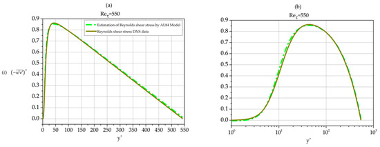
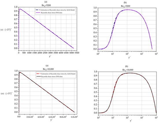
Figure 21.
Normalized Reynolds shear stress profiles. Comparison of AL84-based calculation with DNS data per se. (i) Reτ = 550; (ii) Reτ = 5200; and (iii) Reτ = 10,000. (a) linear–linear plots; (b) semi-log plots.
The approximation is excellent in all three cases. We note that the approximation is best for the moderate Reynolds number 5200 while the agreement between AL84 prediction and DNS data for 10,000 is better than the one for the low Reynolds number case 550.
5. Conclusions
In the first part of the paper, we concentrated on high accuracy DNS datasets in the range 180 10,000. We have identified logarithmic regions in the mean velocity profiles and the corresponding values of the von Kármán constant for each Reynolds number based on the diagnostic function Ξ. Von Kármán constant estimates based on the DNS data range from κ 0.429 for 550 2000 to κ 0.388 for 4179 10,000. Similarly, based on the diagnostic function Γ, we identified the intervals where the power law approximates well the MVP and determined the corresponding exponent as function of the Reynolds number ranges from 1/6 to 1/9.
For the higher order statistics, we have determined the logarithmic regions in the variance profiles of streamwise and spanwise fluctuations and the corresponding values of the Townsend–Perry constants. We have listed logarithmic regions beyond the one expected by the Townsend’s attached eddy hypothesis. In the region 150 450 the variance of the wall-normal fluctuations takes the value 1.30 for 8016 and 10,000. The peak values of the , , , have been approximated as functions of with logarithmic dependence. In contradistinction, the normalized Reynolds shear stress attains a constant value (approximately 0.96) in the interval 100 250 for higher than 8000.
In the second part of the paper, a data-driven model (AL84), developed for ZPG-TBL, is calibrated for pressure-driven channel flow. It is shown that AL84 describes very accurately the mean velocity profile as well as the Reynolds shear stress profile for pressure-driven channel flow. In the framework of AL84 the skin friction coefficient is expressed analytically as function of and, in various comparisons, it is in excellent agreement with DNS data least-squares fits.
The AL84-Model accuracy can be further improved, and its range of applicability can be extended as higher Reynolds number DNS data become available. We expect that the accuracy of the AL84 model will be further enhanced since it incorporates the logarithmic law in the overlap region of the boundary layer which is expected to be approached asymptotically as .
We conclude that, in addition to its pertinence to theoretical developments and in providing guidance in searching for the asymptotic structure of turbulent boundary layers the AL84 model is useful in the development of turbulence models valid very close to solid walls [43,45] as well as in the imposition of boundary conditions near solid surfaces via the wall functions methodology. Furthermore, due to its explicit form, the AL84 model is ideally suited for the imposition of initial conditions in the numerical integration of the parabolized Navier–Stokes equations and Prandtl’s equations for turbulent boundary layers.
Author Contributions
Conceptualization, A.L.; methodology, A.L.; software, A.P.; validation, A.P.; data curation, A.P; writing—original draft, A.L.; visualization, A.P.; supervision, A.L.; funding acquisition, A.L. All authors have read and agreed to the published version of the manuscript.
Funding
This research project was supported by the Hellenic Foundation for Research and Innovation (H.F.R.I.) under the “2nd Call for H.F.R.I. Research Projects to support Faculty Members & Researchers” (Project Number: 4584).
Data Availability Statement
Data are contained within the article.
Conflicts of Interest
The authors declare no conflicts of interest.
References
- Lee, M.; Moser, R.D. Direct numerical simulation of turbulent channel flow up to Reτ = 5200. J. Fluid Mech. 2015, 774, 395–415. [Google Scholar] [CrossRef]
- Bernardini, M.; Pirozzoli, S.; Orlandi, P. Velocity statistics in turbulent channel flow up to Reτ = 4000. J. Fluid Mech. 2014, 742, 171–191. [Google Scholar] [CrossRef]
- Lozano-Durán, A.; Jiménez, J. Effect of the computational domain on direct simulations of turbulent channels up to Reτ = 4200. Phys. Fluids 2014, 26, 011702. [Google Scholar] [CrossRef]
- Yamamoto, Y.; Tsuji, Y. Numerical evidence of logarithmic regions in channel flow at Reτ = 8000. Phys. Rev. Fluids 2018, 3, 012602. [Google Scholar] [CrossRef]
- Hoyas, S.; Oberlack, M.; Alcántara-Ávila, F.; Kraheberger, S.V.; Laux, J. Wall turbulence at high friction Reynolds numbers. Phys. Rev. Fluids 2022, 7, 014602. [Google Scholar] [CrossRef]
- Liakopoulos, A. Explicit representations of the complete velocity profile in a turbulent boundary layer. AIAA J. 1984, 22, 844–846. [Google Scholar] [CrossRef]
- Liakopoulos, A.; Palasis, A. On the Composite Velocity Profile in Zero Pressure Gradient Turbulent Boundary Layer: Comparison with DNS Datasets. Fluids 2023, 8, 260. [Google Scholar] [CrossRef]
- Liakopoulos, A. Fluid Mechanics, 2nd ed.; Tziolas Publications: Thessaloniki, Greece, 2019; ISBN 978-960-418-774-4. (In Greek) [Google Scholar]
- Dean, R.B. Reynolds number dependence of skin friction and other bulk flow variables in two-dimensional rectangular duct flow. J. Fluids Eng. 1978, 100, 215–223. [Google Scholar] [CrossRef]
- Zanoun, E.S.; Nagib, H.; Durst, F. Refined Cf relation for turbulent channels and consequences for high-Re experiments. Fluid Dyn. Res. 2009, 41, 021405. [Google Scholar] [CrossRef]
- Di Nucci, C.; Absi, R. Comparison of Mean Properties of Turbulent Pipe and Channel Flows at Low-to-Moderate Reynolds Numbers. Fluids 2023, 8, 97. [Google Scholar] [CrossRef]
- Millikan, C.B. A Critical discussion of turbulent flows in channels and circular tubes. In Proceedings of the Fifth Internation Congress of Applied Mechanics, Cambridge, MA, USA, 12–16 September 1938. [Google Scholar]
- Landau, L.D.; Lifshitz, E.M. Fluid Mechanics: Course of Theoretical Physics, 2nd ed.; Pergamon Press: Oxford, UK, 1987; Volume 6, ISBN 0-08-033933-6. [Google Scholar]
- Zagarola, M.V.; Smits, A.J. Mean-flow scaling of turbulent pipe flow. J. Fluid Mech. 1998, 373, 33–79. [Google Scholar] [CrossRef]
- McKeon, B.J.; Zagarola, M.V.; Smits, A.J. A new friction factor relationship for fully developed pipe flow. J. Fluid Mech. 2005, 538, 429–443. [Google Scholar] [CrossRef]
- Fiorini, T. Turbulent Pipe Flow-High Resolution Measurements in CICLoPE. Dissertation Thesis, Alma Mater Studiorum Università di Bologna, Forli, Italy, 2017. Available online: http://amsdottorato.unibo.it/8158/1/Fiorini_Tommaso_tesi.pdf (accessed on 4 May 2017).
- Marusic, I.; Monty, J.P.; Hultmark, M.; Smits, A.J. On the logarithmic region in wall turbulence. J. Fluid Mech. 2013, 716, R3. [Google Scholar] [CrossRef]
- Smits, A.J.; McKeon, B.J.; Marusic, I. High-Reynolds number wall turbulence. Annu. Rev. Fluid Mech. 2011, 43, 353–375. [Google Scholar] [CrossRef]
- Oberlack, M. Asymptotic Expansion, Symmetry Groups, and Invariant Solutions of Laminar and Turbulent Wall—Bounded Flows. ZAMM—Zeitschrift für Angewandte Mathematik und Mechanik. J. Appl. Math. Mech. 2000, 80, 791–800. [Google Scholar] [CrossRef]
- Hultmark, M.; Vallikivi, M.; Bailey, S.C.C.; Smits, A.J. Turbulent pipe flow at extreme Reynolds numbers. Phys. Rev. Lett. 2012, 108, 094501. [Google Scholar] [CrossRef] [PubMed]
- Schultz, M.P.; Flack, K.A. Reynolds-number scaling of turbulent channel flow. Phys. Fluids 2013, 25, 025104. [Google Scholar] [CrossRef]
- Palasis, A. Turbulent Boundary Layers: Analysis of DNS Data. Diploma Thesis, Department of Civil Engineering, University of Thessaly, Thessaly, Greece, 31 August 2021. (In Greek). [Google Scholar]
- Barenblatt, G.I.; Chorin, A.J.; Prostokishin, V.M. Scaling laws for fully developed turbulent flow in pipes. Appl. Mech. Rev. 1997, 50, 413–429. [Google Scholar] [CrossRef]
- Barenblatt, G.I.; Chorin, A.J.; Hald, O.H.; Prostokishin, V.M. Structure of the zero-pressure-gradient turbulent boundary layer. Proc. Natl. Acad. Sci. USA 1997, 94, 7817–7819. [Google Scholar] [CrossRef] [PubMed]
- Barenblatt, G.I.; Chorin, A.J.; Prostokishin, V.M. On the problem of turbulent flows in pipes at very large Reynolds numbers. Physics-Uspekhi 2015, 58, 199. [Google Scholar] [CrossRef]
- Zanoun, E.S.; Durst, F.; Nagib, H. Evaluating the law of the wall in two-dimensional fully developed turbulent channel flows. Phys. Fluids 2003, 15, 3079–3089. [Google Scholar] [CrossRef]
- Afzal, N.; Seena, A.; Bushra, A. Friction factor power law with equivalent log law, of a turbulent fully developed flow, in a fully smooth pipe. Z. Für Angew. Math. Und Phys. 2023, 74, 144. [Google Scholar] [CrossRef]
- Monkewitz, P.A.; Nagib, H.M. The hunt for the Kármán ‘constant’ revisited. J. Fluid Mech. 2023, 967, A15. [Google Scholar] [CrossRef]
- Chen, X.; Sreenivasan, K.R. Reynolds number asymptotics of wall-turbulence fluctuations. J. Fluid Mech. 2023, 976, A21. [Google Scholar] [CrossRef]
- Yao, J.; Rezaeiravesh, S.; Schlatter, P.; Hussain, F. Direct numerical simulations of turbulent pipe flow up to Reτ ≈ 5200. J. Fluid Mech. 2023, 956, A18. [Google Scholar] [CrossRef]
- Marusic, I.; Monty, J.P. Attached eddy model of wall turbulence. Annu. Rev. Fluid Mech. 2019, 51, 49–74. [Google Scholar] [CrossRef]
- Laval, J.P.; Vassilicos, J.C.; Foucaut, J.M.; Stanislas, M. Comparison of turbulence profiles in high-Reynolds-number turbulent boundary layers and validation of a predictive model. J. Fluid Mech. 2017, 814, R2. [Google Scholar] [CrossRef]
- Vassilicos, J.C.; Laval, J.P.; Foucaut, J.M.; Stanislas, M. The streamwise turbulence intensity in the intermediate layer of turbulent pipe flow. J. Fluid Mech. 2015, 774, 324–341. [Google Scholar] [CrossRef]
- Meneveau, C.; Marusic, I. Generalized logarithmic law for high-order moments in turbulent boundary layers. J. Fluid Mech. 2013, 719, R1. [Google Scholar] [CrossRef]
- Monty, J.P.; Chong, M.S. Turbulent channel flow: Comparison of streamwise velocity data from experiments and direct numerical simulation. J. Fluid Mech. 2009, 633, 461–474. [Google Scholar] [CrossRef]
- Townsend, A.A.R. The Structure of Turbulent Shear Flow, 2nd ed.; Cambridge University Press: Cambridge, UK, 1976; ISBN 9780521298193. [Google Scholar]
- Chesnokov, Y.G. Influence of the reynolds number on the plane-channel turbulent flow of a fluid. Tech. Phys. 2010, 55, 1741–1747. [Google Scholar] [CrossRef]
- Chesnokov, Y.G. Influence of the Reynolds Number on the Distribution of Turbulent Pulsation Kinetic Energy over a Channel’s Cross Section. Tech. Phys. 2019, 64, 790–795. [Google Scholar] [CrossRef]
- Hoyas, S.; Jiménez, J. Reynolds number effects on the Reynolds-stress budgets in turbulent channels. Phys. Fluids 2008, 20, 101511. [Google Scholar] [CrossRef]
- Landahl, M.T.; Mollo-Christensen, E. Turbulence and Random Processes in Fluid Mechanics, 2nd ed.; Cambridge University Press: Cambridge, UK; New York, NY, USA, 1992; ISBN 978-0521422130. [Google Scholar]
- Coles, D. The law of the wake in the turbulent boundary layer. J. Fluid Mech. 1956, 1, 191–226. [Google Scholar] [CrossRef]
- Yu, M.; Xu, C.X.; Pirozzoli, S. Genuine compressibility effects in wall-bounded turbulence. Phys. Rev. Fluids 2019, 4, 123402. [Google Scholar] [CrossRef]
- De Vanna, F.; Baldan, G.; Picano, F.; Benini, E. On the coupling between wall-modeled LES and immersed boundary method towards applicative compressible flow simulations. Comput. Fluids 2023, 266, 106058. [Google Scholar] [CrossRef]
- Bernardini, M.; Pirozzoli, S. Inner/outer layer interactions in turbulent boundary layers: A refined measure for the large-scale amplitude modulation mechanism. Phys. Fluids 2011, 23, 061701. [Google Scholar] [CrossRef]
- Liakopoulos, A. Computation of high speed turbulent boundary-layer flows using the k–ϵ turbulence model. Int. J. Numer. Methods Fluids 1985, 5, 81–97. [Google Scholar] [CrossRef]

Disclaimer/Publisher’s Note: The statements, opinions and data contained in all publications are solely those of the individual author(s) and contributor(s) and not of MDPI and/or the editor(s). MDPI and/or the editor(s) disclaim responsibility for any injury to people or property resulting from any ideas, methods, instructions or products referred to in the content. |
© 2024 by the authors. Licensee MDPI, Basel, Switzerland. This article is an open access article distributed under the terms and conditions of the Creative Commons Attribution (CC BY) license (https://creativecommons.org/licenses/by/4.0/).