Article

Methods for Parameter Estimation in Wine Fermentation Models

by
Robert Coleman
1,2,*,
James Nelson
1 and
Roger Boulton
1
1
Department of Viticulture and Enology, University of California, Davis, CA 95616, USA
2
Department of Viticulture and Enology, Washington State University, Richland, WA 99164, USA
*
Author to whom correspondence should be addressed.
Fermentation 2024, 10(8), 386; https://doi.org/10.3390/fermentation10080386
Submission received: 19 June 2024 / Revised: 20 July 2024 / Accepted: 24 July 2024 / Published: 27 July 2024
(This article belongs to the Special Issue Modeling, Control and Optimization of Wine Fermentation)

Abstract

:
The estimation of parameters in a wine fermentation model provides the opportunity to predict the rate and concentration outcomes, to strategically intervene to change the conditions, and to forecast the rates of heat and carbon dioxide release. The chosen parameters of the fermentation model are the initial assimilable nitrogen concentration and yeast properties (lag time, viability constant, and specific maintenance rate). This work evaluates six methods for parameter estimation: Bard, Bayesian Optimization, Particle Swarm Optimization, Differential Evolution, Genetic Evolution, and a modified Direct Grid Search technique. The benefits and drawbacks of the parameter computational methods are discussed, as well as a comparison of numerical integration methods (Euler, Runge–Kutta, backward differential formula (BDF), and Adams/BDF). A test set of density-time data for five white and five red commercial wine fermentations across vintage, grape cultivar, fermentation temperature, inoculated yeast strain, and fermentor size was used to evaluate the parameter estimation methods. A Canonical Variate Analysis shows that the estimation methods are not significantly different from each other while, in the parameter space, each of the fermentations were significantly different from each other.

1. Introduction

The need for monitoring, modeling, and controlling wine fermentations is of great economic importance and has been discussed in previous works [1,2,3,4]. Additionally, fermentation (sugar and yeast growth) models have been reviewed and evaluated to meet this need in both research and industry [3,5]. These models consist of sets of nonlinear ordinary differential equations (ODEs) requiring the use of numerical integration and parameter estimation/optimization. Equally, the solutions of the ODEs are not unique; however, as the model equations are based on the fundamental properties of yeast growth, sugar consumption, viability, and nitrogen uptake, the desired solution is determined by parameters bound to ranges of positive values which are supported by published values for Saccharomyces cerevisiae [6,7,8].
A variety of parameter estimation methods have previously been applied to fermentation models: Bard [9], Bayesian Optimization [10], Particle Swarm Optimization [11,12], Differential Evolution [11], Genetic Algorithm [11], and a modified Direct Grid Search technique [13]. These methods fall into general parameter estimation technique categories: gradient search (Bard), sequential design (Bayesian Optimization), bio-inspired or metaheuristic (Particle Swarm Optimization, Differential Evolution, Genetic Algorithm), and brute force (modified Direct Grid Search). Each method and family have their advantages and disadvantages: the ability to find global minima, computer memory space, computational speed, and ease of cloud-based and/or parallelization of computer operation.
With the exception of the Bard method, the integration of the fermentation model ODEs requires a separate (external to parameter estimation) integration method to compute the resulting predicted sugar consumption concentrations. The Euler method, with a uniform time step of an hour, was previously used with the Boulton fermentation model [9]. Alternative higher-order integration formulas, such as the Runge–Kutta, backward differential formula (BDF), and Adams/BDF, sometimes offer superior stability and accuracy. These methods are easily implemented and available through the Python SciPy library [14].
This work will evaluate these alternative estimation methods, as well as provide an initial optimization of the Euler step function when it is applied to the analysis of fermentation patterns. The parameter estimation methods will be compared based on their ability to fit the Boulton model [5,9] against 10 commercial fermentations ranging across vintage, grape cultivar, fermentation temperature, starter yeast, and fermentation volume.

2. Materials and Methods

2.1. Fermentations

Ten commercial fermentations were chosen for this analysis from the 2018, 2019, and 2020 harvest seasons (Treasury Wine Estates, Saint Helena). The fermentations were selected to include an extensive representation varying in vintage, grape cultivar, fermentation temperature, starter yeast, and fermentor size. The attributes of the fermentations are listed in Table 1, and the °Brixtime courses are plotted in Figure 1. The complete datasets for the ten fermentations, including time, temperature, and °Brix, are published in the Supplementary Materials (Table S1).

2.2. Fermentation Model

The density form of the Boulton model was used to evaluate the ten commercial fermentations; this is described in detail elsewhere [5]. The model consists of eight ODEs that are solved using a numerical integration method (i.e., Euler). Four enological parameters (lag time (h), initial nitrogen (mg/L), specific maintenance rate (1/h), and viability constant (L/g/h)) are optimized/fitted against available measurements from the fermentation: sugar consumption time course data (°Brix versus time in hours for this work), fermentation temperature (isothermal for this work), and initial yeast inoculum (g/L). The optimized parameter estimates are returned to the model and integrated to provide the ‘predicted’ fermentation sugar consumption curve (generally known as the “Brix curve”). It should be noted that the Boulton model includes a parameter for ethanol inhibition; however, in this work, this parameter was held constant at 0.035 based on the previous and extensive use of the model and the insensitivity of this parameter’s impact on the final prediction outcome.

2.3. Parameter Estimation Methods

Six parameter estimation methods were compared: Bard (B), Bayesian Optimization with a Sequential Monte Carlo sampler (BO-SMC), Particle Swarm Optimization (PSO), Differential Evolution (DE), Genetic Algorithm (GA), and a modified Direct Grid Search (MDGS). The Bard method, using the Davidon–Fletcher–Powell [15] approach of derivative estimation, is run as a standalone executable software program originally compiled in Fortran [16,17]. The MDGS method runs as Python-based code for this analysis [13]. The remaining methods are run in Python from available statistical packages or online published code: BO-SMC from the ‘PyMC’ library [18], PSO from online code [19], DE from the ‘limfit’ package [20], and GA from the ‘genetic algorithm’ package [21].
As needed per the method type, the methods were provided with an initial guess of the four parameters required by the Boulton model. Additionally, they were all given bounds or extents of the enological parameters based on the fundamental knowledge and experimentation of said parameters (see Supplementary Material—Table S2). The use and value of fundamental parameters was the main reason why machine learning or Artificial Intelligence optimization approaches were not needed in this work.
The Bard method is unique in this set of tested methods as it uses a gradient-based technique for parameter estimation. It is therefore prone to finding local minima or failing to converge based on initial guesses. To overcome this problem, a simple grid search was employed to seed the Bard method with initial guesses of low, middle, and high values based on the given bounds of each parameter. This resulted in running the method 34 = 81 times while evaluating for the best overall fit. The best fit for all methods was determined by minimizing the residuals between the predicted and actual measurements using the residual sum of squares (RSS).
The parameter estimation methods were not optimized for their runtime performance as the goal of this work was to compare the accuracy and precision of methods, not computational performance. The method-, library-, or package-specific options are provided in the Supplementary Materials (Table S3).

2.4. Numerical Integration Methods

The numerical integration methods employed for each of the parameter estimation methods (except for the Bard method) include Euler and those found in the SciPy library: RK45, RK23, DOP853, Radau, BDF, and LSODA [14]. Unlike Euler, these numerical integration methods in the SciPy library are adaptive; therefore, a separate analysis of Euler was performed to provide an initial optimization of step size.
Euler step sizes of 1, 2, 5, 15, 30, 60, 120, and 300 min were tested using the fermentation ID ‘450’ with average parameter estimates from the DE optimization method. The 1 min step size was used as a reference to cross-plot against the remaining larger step sizes. Additionally, the root mean square error (RMSE), mean absolute error (MAE), and percent relative absolute error (%RAE) were calculated against the 1 min step size.
The cross comparison of the numerical integration methods was formulated using a 1 h (60 min) Euler step size against the remaining SciPy methods. The RMSE, MAE, and %RAE were calculated for the predicted sugar consumption curves of fermentation ID ‘450’ as an example. The complete set of fermentation results are summarized in the Supplementary Materials (Table S4).

2.5. Comparison of Parameter Estimation Methods

The measured sugar consumption curves were fitted by each parameter estimation method with the means, standard deviations, and RMSE calculated. To determine statistical significance, one-way MANOVAs were individually carried out on the factors ‘parameter estimation methods’ and ‘Fermentation ID’ (fermentations). Canonical Variate Analysis (CVA) was completed to provide further statistical insight. Comparison analyses were carried out in R [22] and RStudio [23] with the ‘candisc’ package [24].

3. Results

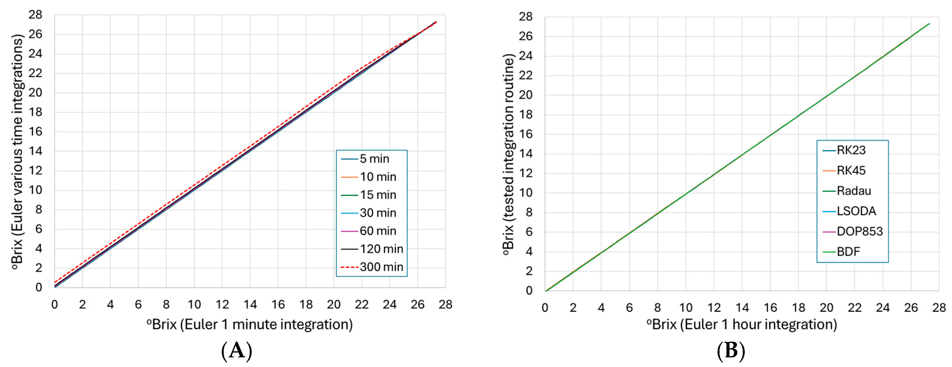
3.1. Analysis of Euler Integration Step Size

To assess the error caused by varying interval step sizes in the Euler integration method, a small uniform step size of 1 min was selected as a benchmark. The resulting paired values (°Brix of 1 min step size versus incrementing step sizes) were evaluated on a cross plot shown in Figure 2A. Step sizes from 5 to 120 min showed no visual change in the 1-to-1 linearity through the x = y line. At a step size of 300 min, the result showed a deviation of the x = y line, indicating a significant truncation error in the integration. To further validate this visual indicator, RMSE, MAE, and %RAE were calculated for each step size against the 1 min step size (Table 2). The %RAE showed a 5.61% error in the 300 min step size; therefore, if a 5% error cutoff is used, one can use up to at least 120 min with acceptable outcomes. Previous unpublished works by the authors have indicated that a 1 h step size has the benefit of minimal error and desirable computational efficiency.

3.2. Analysis of Alternate Integration Methods

To evaluate the performance of alternate numeric integration methods found in the SciPy library, a cross plot of the Euler integration with a step size of 1 h was graphed against the various alternative methods (Figure 2B). Visually, there appears to be no deviation in the methods from the x = y line. Further statistical analysis (Table 3) indicates that the methods’ %RAE were ~1% or less; therefore, it was concluded that any of the numerical integration methods are suitable for the Boulton model for these commercial fermentations. Any subsequent analysis in this work utilized the Euler method with a 1 h integration step size due to its ease of implementation and the convenience of producing whole number hourly outputs.

3.3. Analysis of Parameter Estimation Methods

The RMSE analysis summarized in Table 4 indicates that the magnitude of error between parameter estimation methods was less than the magnitude of error between fermentations. The discrepancy between fermentations was anticipated due to the noise in the °Brix–time course measurements in a commercial winery setting. This noise is visually apparent in Figure 1, with fermentation ID ‘486’ being especially noted at the end of the fermentation. Conversely, the relatively consistent error between parameter estimation methods within a single fermentation provides us with confidence that the methods are fitting the curves similarly.
A more detailed analysis of the methods and the resulting parameter estimates is shown in the means and %RSD in Table 5. Although the RMSE of each fermentation is of similar magnitude, the parameter estimates vary between methods, indicating multiple solutions or optimization minima for the model fitting. This was to be expected given the inherent nature of and criteria used by each parameter estimation method to search for the minimal residual error.
To determine if the parameter estimation methods were significantly different in their estimates, a MANOVA was performed with the parameter estimation method as the factor (p ≤ 0.05). The resulting MANOVA (Supplementary Material—Table S5) was insignificant; therefore, the null hypothesis that the estimates provided by parameter estimation methods are equal across fermentations could not be rejected. This indicates that the parameter estimation methods are using the Boulton model parameters in a similar way to fit the measured fermentation curves.
Given the similarity in the resulting parameter estimates, a review of the means table (Table 5) shows that the DE method often had the lowest relative standard deviation, indicating that it was the method with the highest precision. Additionally, the DE routine had the lowest RMSE or one of the lowest RMSEs in each fermentation, thus indicating its higher accuracy.

3.4. Analysis of Fermentations

The difference in the rates and patterns between the fermentations are apparent in Figure 1. A MANOVA with ‘Fermentation ID’ as the factor (Supplementary Material—Table S6) was significant (p ≤ 0.05), therefore indicating that the parameter estimates of the fermentations were significantly different. Thus, the MANOVA model was used in the CVA and graphed in Figure 3. The first two dimensions of these CVA diagrams (Figure 3A,B) account for 92.4% of the variance ratio within this dataset. The horizontal separation to the right hemisphere is associated with longer lag times in the white fermentations, primarily due to their cooler temperature conditions. The warmer red fermentations and those with higher levels of initial yeast assimilable nitrogen occupy the left hemisphere. The vertical separation is due to the higher maintenance rates and higher viability constants in the lower hemisphere and higher initial assimilable nitrogen in the upper hemisphere. It is interesting to note that the fermentations with higher initial nitrogen levels are also associated in this space with those with lower maintenance rates and viability constants, the two parameters that distinguish the tailing pattern of slow and incomplete fermentations. This pattern has been observed in the more extensive model analysis of commercial fermentations [25], where the enhancement of growth and growth rate by higher assimilable nitrogen levels does not always carry through into more active non-growing cells and higher cell viability.
Regardless of the parameter estimation routines considered, the separation of these ten fermentations based on their parameter values (Figure 3A,B) indicates that the density version of the model (°Brix consumption) [3] can describe their dynamic nature effectively across volume, cultivar, yeast strain, inoculum level, fermentation temperature, and initial composition. This model is unique in its description of non-growing yeast activity and cell viability in the second stage of the fermentations, and this description is confirmed by the success of its application to the fermentation patterns and the parameter estimation in this diverse set of wine fermentations.

4. Discussion

While several alternative parameter estimation methods exist, the large batch-to-batch variation observed in wine fermentations can make online parameter estimation challenging. In general, parameter estimation techniques for nonlinear systems can be separated into gradient methods, sequential design, bio-inspired algorithms, and computational/brute force. In gradient methods, such as Bard, the gradient of the objective function is calculated at each evaluation [16]. The benefit of gradient methods is that the standard deviation for each parameter can be approximated from the Hessian matrix at the last iteration. The standard deviation provides a confidence interval for the solution of each parameter. The performance of gradient methods is dependent on whether the initial guess is close to the global solution. In its application to wine fermentation, there is typically not enough information to select good initial guesses, sometimes requiring multiple iterations to find the global solution.
In bio-inspired algorithms such as PSO, GA, and DE, only lower and upper bounds are provided, making these algorithms attractive for automated parameter estimation across concurrent fermentations; however, these algorithms typically suffer from long computation times. While long computation times are not generally a problem for a single fermentation, at the winery scale, long computation times make cloud implementation more complex as tasks must be queued and executed asynchronously instead of being performed on demand.
In Bayesian estimation methods such as BO-SMC, the system model, measurement model, state noise, and measurement noise are determined a priori [26]. When estimating the unknown parameters, it is necessary to account for the state and measurement noises, which are often computationally intensive and a source of convergence difficulties [26].
Brute force methods such as MDGS are typically limited in the range and number of parameters; however, the computations can be performed in parallel across processors. The results in this work show that all parameter estimation methods converged to similar solutions; therefore, a method should be selected for its ability to handle large batch-to-batch variation and its ease of implementation.
Machine learning has also been used to develop models and predictions of biological processes where the underlying mechanics are unknown [27,28,29,30]; however, the coefficients and biases generally have no relationship or meaning concerning the underlying process, making the interpretation of results less meaningful. For this reason, these approaches were not considered in this work.
The lack of significant differences between the parameter estimation methods and integration routines suggest that the focus should be on improving density measurements (i.e., density sensors, methods, and placement), as well as improving first principle model descriptions of non-growing cells’ activity and their decline. Given the slow rates of change in wine fermentations, the speed of the parameter estimation method is generally not a limitation. What is important is that the parameter estimation method should be robust and require little or no human intervention to adjust the bounds or initial guesses. In turn, the selection of a parameter estimation method becomes a choice of the user’s ultimate need: robust/no human intervention, memory space, and/or processor time or computing efficiency.

5. Conclusions

All the parameter estimation methods considered produced satisfactory parameter values. There was no significant difference between the methods in the parameter space of a diverse fermentation dataset. In contrast, each fermentation was significantly different from the others in the parameter space.

Supplementary Materials

The following supporting information can be downloaded at: https://www.mdpi.com/article/10.3390/fermentation10080386/s1, Table S1: Ten commercial fermentations °Brix, temperature and time data; Table S2: Parameter bounds; Table S3: Method-, library-, or package-specific options; Table S4: Numerical integration comparison across methods and fermentations; Table S5: MANOVA for estimated parameters and parameter optimization methods; Table S6: MANOVA for estimated parameters and ten commercial fermentations.

Author Contributions

Conceptualization, R.C., J.N. and R.B.; methodology, R.C., J.N. and R.B.; software, R.C., J.N. and R.B.; validation, R.C., J.N. and R.B.; formal analysis, R.C., J.N. and R.B.; investigation, R.C., J.N. and R.B.; data curation, R.C.; writing—original draft preparation, R.C.; writing—review and editing, R.C., J.N. and R.B.; visualization, R.C.; supervision, R.B. All authors have read and agreed to the published version of the manuscript.

Funding

The Stephen Sinclair Scott Endowment (R.B.) and Rodgers University Fellowship in Electrical and Computer Engineering (J.N.).

Institutional Review Board Statement

Not applicable.

Informed Consent Statement

Not applicable.

Data Availability Statement

Data are available upon request.

Acknowledgments

Treasury Wine Estates, Saint Helena, CA.

Conflicts of Interest

The authors declare no conflicts of interest.

References

  1. Knoesen, A.; Boutlon, R. A Brief History of the Modeling, Control and Optimization of Wine. Fermentation, 2024; in submission. [Google Scholar]
  2. Boulton, R.B.; Singleton, V.L.; Bisson, L.F.; Kunkee, R.E. Principles and Practices of Winemaking; Chapman & Hall: New York, NY, USA; Springer: Boston, MA, USA, 1996; ISBN 0-412-06411-1. [Google Scholar] [CrossRef]
  3. Marín, M.R. Alcoholic Fermentation Modelling: Current State and Perspectives. Am. J. Enol. Vitic. 1999, 50, 166–178. [Google Scholar] [CrossRef]
  4. Bisson, L.F.; Butzke, C.E. Diagnosis and Rectification of Stuck and Sluggish Fermentations. Am. J. Enol. Vitic. 2000, 51, 168–177. [Google Scholar] [CrossRef]
  5. Nelson, J.; Boulton, R. Models for Wine Fermentation and Their Suitability for Commercial Applications. Fermentation 2024, 10, 269. [Google Scholar] [CrossRef]
  6. Pirt, S.J. Principles of Microbe and Cell Cultivation; Wiley: New York, NY, USA, 1975; ISBN 0470690380, 9780470690383. [Google Scholar]
  7. Aiba, S.; Humphrey, A.E.; Millis, N.F. Biochemical Engineering, 2nd ed.; Academic Press: New York, NY, USA, 1973; ISBN 0-12-045052-6.1. [Google Scholar]
  8. Bailey, J.E. Biochemical Engineering Fundamentals; McGraw Hill: New York, NY, USA, 1977; ISBN 0-07-003210-6. [Google Scholar]
  9. Boulton, R. The Prediction of Fermentation Behavior by a Kinetic Model. Am. J. Enol. Vitic. 1980, 31, 40–45. [Google Scholar] [CrossRef]
  10. Coleman, M.C.; Fish, R.; Block, D.E. Temperature-Dependent Kinetic Model for Nitrogen-Limited Wine Fermentations. Appl. Environ. Microbiol. 2007, 73, 5875–5884. [Google Scholar] [CrossRef] [PubMed]
  11. Coleman, R.E.; Boulton, R.B. Alternative Estimation Routines for Modeling and Prediction of Commerical Wine Fermentations. In Proceedings of the 72nd American Society of Enology and Viticulture National Conference, Virtual, 24 June 2021. [Google Scholar]
  12. AWRI. Fermentation Simulator. Available online: https://www.awri.com.au/industry_support/winemaking_resources/wine_fermentation/awri-ferment-simulator/ (accessed on 18 May 2024).
  13. Nelson, J.N. The Digitization of Wine Fermentation. Ph.D. Thesis, University of California Davis, Davis, CA, USA, 2023. [Google Scholar]
  14. Virtanen, P.; Gommers, R.; Oliphant, T.E.; Haberland, M.; Reddy, T.; Cournapeau, D.; Burovski, E.; Peterson, P.; Weckesser, W.; Bright, J.; et al. Scipy 1.0: Fundamental Algorithms for Scientific Computing in Python. Nat. Methods 2020, 17, 261–272. [Google Scholar] [CrossRef] [PubMed]
  15. Fletcher, R.; Powell, M.J.D. A Rapidly Convergent Descent Method for Minimization. Comput. J. 1963, 6, 163–168. [Google Scholar] [CrossRef]
  16. Bard, Y. Comparison of Gradient Methods for the Solution of Nonlinear Parameter Estimation Problems. SIAM J. Numer. Anal. 1970, 7, 157–186. [Google Scholar] [CrossRef]
  17. Bard, Y. Nonlinear Parameter Estimation; Academic Press: New York, NY, USA, 1974; ISBN 0-12-078250-2. [Google Scholar]
  18. Abril-Pla, O.; Andreani, V.; Carroll, C.; Dong, L.; Fonnesbeck, C.J.; Kochurov, M.; Kumar, R.; Lao, J.; Luhmann, C.C.; Martin, O.A.; et al. Pymc: A Modern, and Comprehensive Probabilistic Programming Framework in Python. PeerJ Comput. Sci. 2023, 9, e1516. [Google Scholar] [CrossRef] [PubMed]
  19. Rahmadya. Particle Swarm. Available online: https://rahmadya.com/2020/05/31/particle-swarm-optimization-in-jupyter-notebook/ (accessed on 18 May 2024).
  20. Newville, M.; Stensitzki, T.; Allen, D.B.; Ingargiola, A. Lmfit: Non-Linear Least-Square Minimization and Curve-Fitting for Python (0.8.0). Zendo. 2014. Available online: https://zenodo.org/records/10998841 (accessed on 11 February 2024).
  21. Python Package Index—Pypi. Python Software Foundation. Available online: https://pypi.org/ (accessed on 12 February 2024).
  22. R Core Team. R: A Language and Environment for Statistical Computing; R Foundation for Statistical Computing: Vienna, Austria, 2023; Available online: https://www.R-project.org/ (accessed on 1 December 2023).
  23. RStudio Team. Rstudio: Integrated Development Environment for R; RStudio, PBC: Boston, MA, USA, 2023; Available online: http://www.rstudio.com/ (accessed on 1 December 2023).
  24. Friendly, M.; Fox, J. Candisc: Visualization Generalized Canonical Correlation Analysis. R. Package Version 0.9.0. 2024. Available online: https://CRAN.R-project.org/package=heplots (accessed on 6 November 2021).
  25. Nelson, J.; Coleman, R.; Gravesen, P.; Silacci, M.; Velasquez, A.; Marinell, K. Analysis of a Commercial Red Wine Fermentation Dataset with a Wine Kinetic Model. Fermentation, 2024; in submission. [Google Scholar]
  26. Shyam, M.M.; Naik, N.; Gemson, R.M.O.; Ananthasayanam, M.R. Introduction to the Kalman Filter and Tuning Its Statistics for near Optimal Estimates and Cramer Rao Bound. arXiv 2015, arXiv:1503.04313. [Google Scholar] [CrossRef]
  27. Zheng, J.; Ma, L.; Wu, Y.; Ye, L.; Shen, F. Nonlinear Dynamic Soft Sensor Development with a Supervised Hybrid Cnn-Lstm Network for Industrial Processes. ACS Omega 2022, 7, 16653–16664. [Google Scholar] [CrossRef] [PubMed]
  28. Gu, X.; Wang, S. Bayesian Takagi–Sugeno–Kang Fuzzy Model and Its Joint Learning of Structure Identification and Parameter Estimation. IEEE Trans Ind. Inform. 2018, 14, 5327–5337. [Google Scholar] [CrossRef]
  29. Moya Almeida, V.; Diezma Iglesias, B.; Correa Hernando, E.C. Artificial Neural Networks and Gompertz Functions for Modelling and Prediction of Solvents Produced by the S. Cerevisiae Safale S04 Yeast. Fermentation 2021, 7, 217. [Google Scholar] [CrossRef]
  30. Florea, A.; Sipos, A.; Stoisor, M.-C. Applying Ai Tools for Modeling, Predicting and Managing the White Wine Fermentation Process. Fermentation 2022, 8, 137. [Google Scholar] [CrossRef]
Figure 1. Brix–time plots of ten commercial fermentations. Time at 0 h is the point of yeast inoculation.
Fermentation 10 00386 g001
Figure 2. Cross plots of numerical integration methods using fermentation ID ‘450’ and the average parameter estimates optimized by the Differential Evolution method. (A) Integrated °Brix values at a Euler step size of 1 min versus Euler step sizes of 5, 10, 15, 30, 60, 120, or 300 min; (B) Comparison of °Brix at a 1 h (60 min) Euler step size versus the integration methods from the SciPy library. There was no observed difference in the Euler step sizes from 5 to 120 min; also, there was no observed difference in the 6 integration methods compared to a 60 min Euler.
Fermentation 10 00386 g002
Figure 3. The CVA of parameter estimations effects’ on the ten fermentations: (A) Loadings plot of parameter estimates; (B) Score plots of the 10 fermentations.
Fermentation 10 00386 g003
Table 1. Attributes of the ten commercial fermentations.
IDVintageCultivarInoculum (g/L)Temperature (°C) 1YeastVolume
(kL)
417A2018Chardonnay0.25818.95VL19.16
417B2019Riesling0.24313.85VL15.43
4502020Cabernet Sauvignon0.24725.85BDX11.30
4572020Cabernet Sauvignon0.24229.15BO21311.53
4862020Syrah0.32127.25M29.82
4892020Cabernet Sauvignon0.24327.95FX1013.57
5712019Sauvignon blanc0.24013.35VL34.54
8232020Sauvignon blanc 0.27014.25VL34.38
8262020Pinot noir0.21124.65RC2122.55
8292019Muscat0.26513.65VL34.11
1 An average temperature (isothermal) was used in the parameter optimization analysis. The temperature data are available in the Supplementary Materials (Table S1).
Table 2. Statistical analysis of incrementing step sizes on the Euler integration method.
Euler Integration Step Size (minutes)
510153060120300
RSME0.0060.0140.0220.0460.0950.1950.513
MAE0.0060.0140.0210.0440.0910.1860.489
%RAE0.070.160.250.151.052.165.61
Table 3. Statistical analysis of alternative integration methods versus a 1 h Euler step size.
Numerical Integration Method
RK23RK45RadauLSODADOP853BDF
RSME0.1020.0660.0920.0970.0940.096
MAE0.0970.0570.0880.0930.0900.092
%RAE1.130.661.021.081.051.07
Table 4. Root mean squared error by method for each fermentation.
ID: 417A417B450457486489571823826829
Root Mean Squared Error (RMSE)
B0.4810.0790.4460.3140.5160.2680.0770.2400.3380.104
BO-SMC0.4990.1670.4870.3240.5150.3120.0900.2520.3380.140
DE0.4770.1120.4560.3140.5100.3030.0820.2410.3260.137
GA0.4790.1290.4850.3280.5120.3060.0900.2430.3300.144
PSO0.4800.1290.4690.3180.5230.3090.1150.2600.3610.161
MDGS0.4870.1510.5000.3500.5550.3630.1310.2700.3730.181
mean0.4840.1280.4740.3250.5220.3100.0980.2510.3440.145
Table 5. Means table with percent relative standard deviation (%RSD) for parameter estimates by method for each fermentation ID.
Lag Time (hours)
ID:417A417B450457486489571823826829
MethodMean ± %RSD
B41.7 ± 12.568.0 ± 1.913.1 ± 3.727.9 ± 3.920.9 ± 2.412.9 ± 5.062.6 ± 1.663.4 ± 5.216.8 ± 6.446.9 ± 2.2
BO-SMC35.2 ± 0.363.2 ± 2.015.3 ± 8.725.6 ± 1.518.5 ± 0.910.8 ± 3.662.9 ± 2.258.1 ± 0.57.6 ± 9.950.3 ± 0.0
DE35.7 ± 0.072.0 ± 0.011.3 ± 0.025.3 ± 0.018.8 ± 0.09.8 ± 0.065.2 ± 0.063.3 ± 0.06.5 ± 0.050.5 ± 0.3
GA33.7 ± 8.169.2 ± 3.614.9 ± 19.726.8 ± 4.218.7 ± 2.79.3 ± 4.764.2 ± 3.861.0 ± 2.66.4 ± 14.752.8 ± 1.9
PSO36.4 ± 3.070.2 ± 4.410.6 ± 10.925.8 ± 3.120.1 ± 0.910.3 ± 8.769.3 ± 6.764.5 ± 10.24.6 ± 87.351.8 ± 6.6
MDGS36.3 ± 10.868.1 ± 3.013.3 ± 24.425.9 ± 6.319.8 ± 3.710.5 ± 23.464.9 ± 4.756.4 ± 3.77.4 ± 38.549.9 ± 10.9
Initial Nitrogen (mg/L)
ID:417A417B450457486489571823826829
MethodMean ± %RSD
B131 ± 9.3158 ± 1.0126 ± 0.2209 ± 4.5320 ± 0.6214 ± 2.4164 ± 1.3145 ± 2.4238 ± 3.4189 ± 0.7
BO-SMC144 ± 0.5136 ± 1.2149 ± 4.3230 ± 2.2327 ± 0.7243 ± 1.9156 ± 1.9135 ± 0.3305 ± 2.9182 ± 0.0
DE145 ± 0.0150 ± 0.0132 ± 0.0226 ± 0.0333 ± 0.0233 ± 0.0161 ± 0.1141 ± 0.0294 ± 0.0182 ± 0.3
GA139 ± 5.1143 ± 3.3148 ± 8.7244 ± 6.3332 ± 2.2230 ± 1.4158 ± 3.8137 ± 2.3291 ± 3.4188 ± 1.2
PSO143 ± 1.5145 ± 4.3133 ± 0.4232 ± 4.8350 ± 0.0235 ± 1.9169 ± 6.0143 ± 7.1282 ± 7.8185 ± 6.2
MDGS150 ± 5.8145 ± 1.9139 ± 6.3235 ± 9.3322 ± 3.5227 ± 7.7161 ± 5.3136 ± 4.4293 ± 6.6184 ± 4.6
Specific Maintenance Rate (1/h)
ID:417A417B450457486489571823826829
MethodMean ± %RSD
B0.169 ± 13.70.129 ± 2.00.300 ± 0.60.224 ± 8.80.081 ± 1.90.200 ± 4.90.144 ± 2.70.143 ± 6.00.126 ± 7.10.121 ± 1.7
BO-SMC0.175 ± 1.10.159 ± 2.00.256 ± 6.40.217 ± 4.20.084 ± 2.30.180 ± 4.40.154 ± 3.50.153 ± 0.40.101 ± 8.30.124 ± 0.1
DE0.171 ± 0.00.133 ± 0.10.300 ± 0.00.221 ± 0.00.079 ± 0.00.196 ± 0.00.146 ± 0.40.143 ± 0.00.111 ± 0.00.124 ± 0.6
GA0.183 ± 8.00.147 ± 5.70.261 ± 11.30.192 ± 12.70.079 ± 6.90.198 ± 2.10.151 ± 7.80.150 ± 3.90.115 ± 8.80.116 ± 2.4
PSO0.176 ± 2.90.144 ± 9.00.300 ± 0.00.210 ± 9.60.067 ± 1.80.194 ± 1.70.134 ± 12.20.140 ± 10.70.123 ± 19.20.122 ± 13.2
MDGS0.162 ± 10.10.141 ± 4.00.281 ± 7.30.207 ± 19.20.091 ± 16.90.209 ± 17.30.142 ± 11.00.149 ± 9.10.114 ± 17.80.120 ± 9.9
Viability Constant (L/g/h)
ID:417A417B450457486489571823826829
MethodMean ± %RSD
B20.2 ± 3.229.3 ± 2.927.9 ± 0.419.3 ± 2.622.4 ± 1.118.5 ± 1.918.3 ± 2.923.7 ± 4.725.8 ± 2.015.8 ± 1.8
BO-SMC17.4 ± 0.325.0 ± 2.426.4 ± 0.217.9 ± 0.221.4 ± 0.617.1 ± 0.318.3 ± 2.023.8 ± 0.720.0 ± 1.816.6 ± 0.1
DE17.3 ± 0.029.3 ± 0.126.5 ± 0.017.9 ± 0.021.7 ± 0.017.0 ± 0.018.8 ± 0.923.8 ± 0.019.6 ± 0.016.5 ± 0.6
GA17.2 ± 0.425.6 ± 4.426.3 ± 0.418.0 ± 1.821.8 ± 1.517.2 ± 0.918.6 ± 6.723.3 ± 2.419.4 ± 1.517.0 ± 1.6
PSO17.0 ± 1.826.0 ± 12.226.4 ± 0.718.0 ± 1.322.4 ± 1.816.8 ± 2.120.8 ± 9.924.8 ± 2.219.7 ± 2.616.6 ± 9.1
MDGS17.5 ± 3.528.8 ± 3.826.6 ± 2.318.2 ± 3.920.7 ± 8.716.8 ± 5.021.6 ± 9.924.5 ± 11.719.4 ± 3.117.9 ± 6.3
Disclaimer/Publisher’s Note: The statements, opinions and data contained in all publications are solely those of the individual author(s) and contributor(s) and not of MDPI and/or the editor(s). MDPI and/or the editor(s) disclaim responsibility for any injury to people or property resulting from any ideas, methods, instructions or products referred to in the content.

