Article

Selection of Spectral Parameters and Optimization of Estimation Models for Soil Total Nitrogen Content during Fertilization Period in Apple Orchards

1
College of Resources and Environment, Shandong Agricultural University, Tai’an 271018, China
2
Shandong Yuanhong Survey Planning and Design Co., Ltd., Jinan 250014, China
3
Jinan Survey and Mapping Research Institute, Jinan 250101, China
*
Authors to whom correspondence should be addressed.
These authors contributed equally to this work.
Horticulturae 2024, 10(4), 358; https://doi.org/10.3390/horticulturae10040358
Submission received: 11 March 2024 / Revised: 31 March 2024 / Accepted: 2 April 2024 / Published: 4 April 2024

Abstract

:
The rapid and accurate diagnosis of nitrogen content in apple orchard soil is of great significance for the rational application of nitrogen fertilizer in orchards to improve apple yield and quality. An apple orchard in Shuangquan Town, Changqing District, Jinan City, Shandong Province, was taken as the experimental area. The optimal method for extracting spectral characteristic bands and screening spectral characteristic indices (SCIs) of soil total nitrogen (TN) for independent and comprehensive fertilization periods was explored. Independent and comprehensive soil TN content estimation models were constructed and optimized for each and the entire fertilization period, respectively. The results show that compared with the correlation coefficient method, stepwise multiple linear regression (SMLR) performs better in extracting hyperspectral characteristic bands of soil TN content. It helps to achieve a higher modeling accuracy, smaller root mean square error (RMSE), and is more conducive to avoiding the influence of multicollinearity of model variables. The sensitive areas of soil TN content in the SCI do not undergo significant changes due to different fertilization periods. Among them, the ratio spectral indices (RSIs) are in the range of 800–900 nm, 1900–1950 nm, and 2200–2300 nm, while the sensitive areas of the difference spectral index (DI) and Normalized difference spectral index (NDSI) are in the range of 1900–1950 nm and 2200–2300 nm. The combination of SCI and characteristic bands significantly improves the prediction accuracy of soil TN estimation models. The independent and comprehensive estimation models for each fertilization period based on the BP (back propagation) neural network optimized by the Mind Evolution Algorithm (MEA-BPNN) can achieve a more stable and accurate estimation of soil TN. Finally, using soil spectral characteristic bands selected through continuum removal (CR) transformation and SMLR, combined with SCI, the model based on the MEA-BPNN (CR-SCI-MEA-BPNN) has the best prediction performance. The modeling determination coefficients R2 for each fertilization period reached 0.94, 0.95, 0.92, and 0.94, respectively, with RMSE of 0.0032, 0.0024, 0.0035, and 0.0027. The R2 and RMSE of the modeling and validation set of the entire fertilization period comprehensive model are 0.899, 0.0038, and 0.89, 0.0041, respectively. The results of this article provide technical support for promoting the timely monitoring of soil TN content and guiding rational fertilization in apple orchards.

1. Introduction

Apple is one of the four major fruits in the world, cultivated in over 80 countries worldwide. China is the world’s largest producer and consumer of apples. According to the 2022 China Apple Industry Report released by the China Apple Industry Association, the national planting area in 2022 was 2 million hectares, with a total production of 45.9734 million tons, which accounted for 58.3% of the global total production [1]. Nitrogen is an essential nutrient for maintaining the growth of apple trees [2], and plays an irreplaceable role in organ development, material metabolism, fruit quality, and yield [3,4,5,6,7]. Soil nitrogen is the main source of nutrients for fruit trees, and its content is the basis for orchard fertilization and an important indicator for evaluating and managing orchard quality [6]. Due to the challenge of estimating the nitrogen content of orchard soil in advance, fruit farmers often apply too much or too little nitrogen in their application of nitrogen fertilizer in orchards. This leads to the abnormal growth of fruit trees, susceptibility to diseases, and soil and groundwater pollution [8]. Therefore, knowing how to diagnose the soil nitrogen in apple orchards quickly and accurately is of great significance for the timely monitoring and scientific management of reasonable nitrogen application to improve yield and quality [2,3,4].
At present, in the monitoring of soil nitrogen in apple orchards, the laboratory Kjeldahl nitrogen determination method is commonly used to determine the soil total nitrogen (TN) content. Although it can be highly accurate, the experimental steps are cumbersome, especially the drawbacks of sampling causing significant damage to soil and roots [9], which greatly limits its application in practice. The emergence of hyperspectral remote sensing technology provides a new way for non-destructive estimation of soil nutrients, which has advantages such as being fast, accurate, non-destructive, and pollution-free. It is widely used in the estimation and inversion of soil physicochemical properties [10,11]. Hyperspectral inversion has achieved good research results in soil iron oxides [12], organic carbon [13,14], organic matter [10,15,16], and soil moisture content [17], providing a reference for the rapid monitoring of soil nitrogen in orchards.
In recent years, scholars at home and abroad have conducted extensive research on spectral estimation techniques for soil TN content and found that the spectral corresponding characteristics of soil TN content are mainly concentrated in the visible near-infrared region [18,19,20]. Multiple modeling methods have been attempted to prove the feasibility of quantitative inversion of soil TN spectra [21,22,23]. Niu et al. constructed a hyperspectral estimation model for TN content in Shajiang black soil and found that the accuracy of the SVM model was slightly higher than that of the indices model, but both models could facilitate the rapid estimation of TN content in Shajiang black soil [24]. The spectral estimation technology of soil nutrients has achieved some preliminary results in the research in apple orchards [25,26], navel orange orchards [27], and rubber orchards [28]. Liu et al. constructed an estimation model for soil organic matter content in apple orchards using the random forest method, and the R2 of the modeling sample set reached 0.88 [29]. Tang et al. extracted hyperspectral features of rubber plantation soil using the successive projection algorithm (SPA) and established a partial least squares regression (PLSR) model for soil TN content [30]. Liu et al. used the competitive adaptive reweighting algorithm (CARS), SPA, and CARS-SPA algorithm to select the characteristic bands of soil TN spectrum. The SVM model established using the characteristic wavelengths selected by the CARS method had the best performance [31]. Overall, most spectral inversion methods for nitrogen content in orchard soil currently used conventional spectral transformation and correlation analysis to screen characteristic bands, and based on this, commonly used regression models were constructed. There is a lack of in-depth exploration of soil spectral information, which affects the predictive performance of the models. And there is a lack of systematic analysis and screening of data processing methods. In addition, existing research often randomly selected a certain point in the year for sample collection, and the model lacked a duration test, resulting in low practicality of the model.
The purpose of this study is as follows: (i) Screen the optimal soil spectra characteristic band extraction method for soil TN during each fertilization period; (ii) select the most suitable soil TN spectral characteristic index (SCI); (iii) construct and optimize independent and comprehensive soil TN estimation models for each fertilization period and the entire fertilization period, respectively. The layout of this article is as follows: firstly, collect and transform the soil spectral reflectance for each fertilization stage; then, conduct in-depth research step by step according to the order of the three objectives mentioned above.

2. Materials and Methods

2.1. Data Acquisition

2.1.1. Overview of Experimental Orchard

The experimental orchard is located at the foot of a hill in Shuangquan Town, Changqing District, Jinan City, Shandong Province, China, with an area of approximately 33 hm2 (116.7426–116.7507° E, 36.3139–36.3216° N). It is located at the northwest foot of Mountain Taishan, and the soil type is brown soil. The apple tree spacing is 1.5 m, the row spacing is 4.5 m, the number of plants per 667 m2 is about 100, the crown width is 1–1.5 m, and the overall canopy closure of the orchard is about 0.6. Apple varieties include Gala and Fuji, with an age of about 5 years. During the 4 stages of apple growth: young fruit (in early May, young fruit formation with slower growth), swelling (in mid-June, fruit volume rapidly increases, the flesh thickens, and the skin color lightens), quality (in mid-July, fruit volume is basically fixed, and the color and taste are formed), and postpartum (in early October, after fruit picking, the roots grow at its peak before winter) period, nitrogen fertilizer is applied using drip irrigation, respectively.

2.1.2. Soil Sample Collection and Analysis

The experimental orchard was divided into modeling and validation areas, with 100 and 40 sampling points evenly distributed, respectively, and a fruit tree was selected as the center of each sampling point. Soil samples were collected 10 days before each of the 4 fertilization dates. To ensure the collection of soil as close as possible to the capillary roots and reduce damage to fruit trees during sampling, a soil drill was used to collect mixed soil samples from 0 to 30 cm below the soil surface at a distance of 30 cm horizontally from the apple tree roots [31]. Sand, gravel, and animal and plant residues were removed from the collected soil samples. Soil samples were placed in a dry and ventilated place for natural air drying. During the airdrying process, the samples were kept clean and not contaminated with each other. Then, the samples were ground through a 60-mesh sieve and mixed evenly before being divided into two parts using the quartering method. One sample was used to determine the soil TN content using the micro Kjeldahl nitrogen determination method (Table 1). Another one was placed in a completely black container (diameter 10 cm, depth 2 cm, default infinite depth) for obtaining soil spectral data.

2.1.3. Soil Spectral Collection

The collection of soil spectral data was carried out outdoors in an open and unobstructed area with artificial control of the surrounding environment, using natural sunlight as the light source. The ASD Fieldspec3 ground object spectrometer was adopted, with a spectral range of 350–2500 nm and a resampling interval of 1 nm for data output. A total of 2151 bands of reflectance were collected. To ensure the solar altitude angle, measurements were taken from 10:00 to 14:00. When measuring, the dish filled with the soil sample to be tested was placed on black rubber with a field of view angle of 25° and a distance of 15 cm from the soil sample. To reduce the influence of soil spectral anisotropy [32], each soil sample was rotated at 90° three times during measurement, and a total of 20 spectral curves were collected in each direction. After arithmetic averaging, the reflectance spectrum of the sample was obtained. During the measurement process, a white board with a reflectivity of 1 was used for calibration in a timely manner [33].

2.1.4. Spectral Data Preprocessing

On the basis of breakpoint correction, edge noise removal, and SG smoothing, the original soil spectral reflectance (R) was transformed into eight forms: reciprocal (1/R), logarithmic (LogR), square root ( R ), first-order derivative [(R)′], reciprocal first-order derivative [(1/R)′], logarithmic first-order derivative [(LogR)′], square root first-order derivative [( R )′], and continuum removal (CR). The transformation result data were used together with the original spectrum as modeling and analysis data.

2.2. Modeling Parameter Screening

2.2.1. Characteristic Band Screening

  • Correlation coefficient method
Correlation analysis band by band was performed between the TN content of the sample soil and the original soil reflectance, as well as various transformations. The bands at the extreme or sudden change point of the correlation coefficient were selected as the characteristic bands [34]. The commonly used Pearson coefficient was selected as the correlation coefficient, and the calculation formula is as follows:
r i = n = 1 N ( R n i R i ¯ ) ( T N n T N ¯ ) n = 1 N ( R n i R i ¯ ) 2 n = 1 N T N n T N ¯
where ri represents the correlation coefficient between soil TN content and input spectrum and i is the band number; R is the input spectrum; Rni represents the input value of the nth sample at the i-th band; R i ¯ represents the mean of the input spectral values of all soil samples in the i-th band; TNn is the soil TN content of the nth soil sample; T N ¯ is the average TN content of all soil samples.
2.
Stepwise multiple linear regression (SMLR)
The spectral data of the original soil reflectance and its various transformation forms in the range of 400–2450 nm were taken as the input spectrum, and the SMLR method was used to screen the characteristic bands of soil TN content. The basic operation steps were divided into two steps: first, variables that have not been tested as significant based on a certain level of significance were eliminated; second, new variables were introduced into the regression model [35]. The representation of the filtering model is as follows:
T N = a 0 + n = 1 N a i R i
where TN represents the soil TN content, a0 and ai are the constant terms and coefficients of the regression model, N is the number of filtered bands, and Ri is the input spectral value of the wavelength at the i-th modeling band.

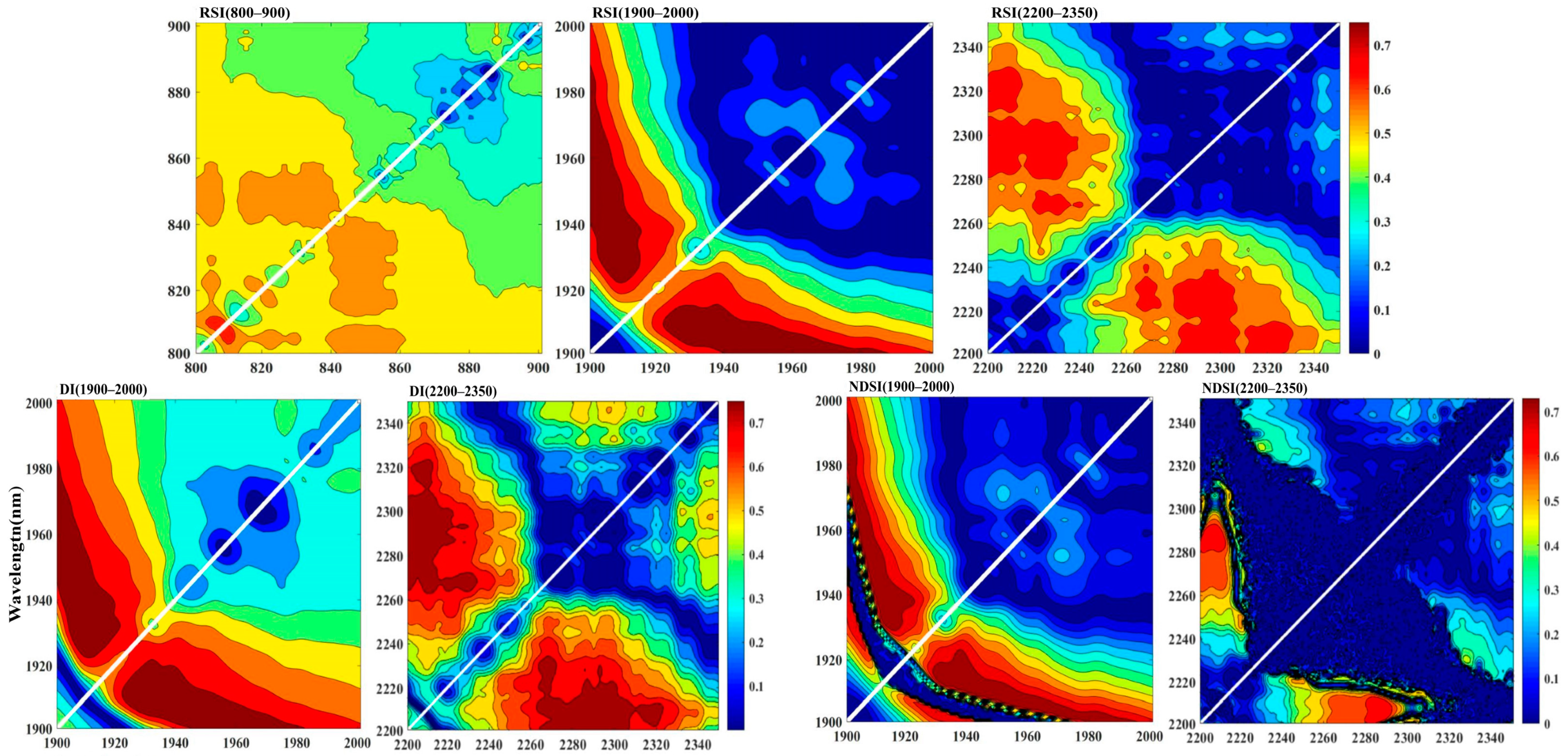
2.2.2. Spectral Characteristic Index (SCI) Screening

In the range of 400–2450 nm, SCIs were calculated for the original soil spectra of each fertilization period band by band [36], and different spectral index matrices were obtained for the entire band range; SCI included the ratio spectral index (RSI), difference spectral index (DI), and Normalized difference spectral index (NDSI). A correlation coefficient matrix was obtained through performing correlation analysis with soil TN content and analyzed by using contour maps [37]. Then, the SCIs for the sensitive areas of soil TN content was analyzed, the combination of SCI with high correlation with soil TN were screened and determined.
The formulas for RSI, DI, and NDSI are as follows:
R S I ( R 1 , R 2 ) = R 1 / R 2 ,
D I ( R 1 , R 2 ) = R 1 R 2 ,
N D S I ( R 1 , R 2 ) = ( R 1 + R 2 ) / ( R 1 R 2 ) ,
where R1 and R2 represent the spectral reflectance of any two bands in the sample spectrum.

2.3. Modeling Methods

Firstly, R and its 8 transformations during each fertilization period were used as input spectra, respectively, and the soil TN characteristic bands were extracted based on correlation coefficient method and SMLR method, respectively. Afterwards, the modeling effects of univariate regression and MLR, as well as the MEA-BPNN method (Back propagation neural network optimized by Mind Evolution Algorithm) were compared. Subsequently, the optimal characteristic bands extraction method was selected based on the model’s coefficient of determination (R2) and root mean square error (RMSE). Then, using band by band analysis techniques and correlation analysis methods, the sensitive areas of soil TN spectral index were determined, and SCIs with high correlation with soil TN were screened out. Finally, based on SCIs and characteristic bands combinations, MLR and MEA-BPNN methods were used to construct and optimize independent and comprehensive soil TN content estimation models for each fertilization period, and the optimal models were validated. The above steps were implemented using MATLAB (version: 2016b) software.

2.3.1. Regression Analysis

Univariate regression is used for regression analysis that includes only one independent variable and one dependent variable [38]. MLR is the most common method for the quantitative relationship analysis between multiple variables [39]. The calculation method is as follows:
T N = T N 1 T N 2 T N 3 T N n , R = R 11 R 12 R 13 R 1 m R 21 R 22 R 23 R 2 m R 31 R 32 R 33 R 3 m R n 1 R n 2 R n 3 R n m ,
where TN is the TN content value of the soil sample and R is the spectral characteristic band matrix of the soil sample; TNi refers to the TN content of the i-th soil sample; Rij (i = 1, 2, 3… n; j = 1, 2, 3… m) represents the reflectance value of the i-th sample at the j-th characteristic band; n is the soil sample capacity, i.e., the number of samples; and m is the number of characteristic bands.
Assuming that the soil TN value can be expressed linearly by Ri (i = 1, 2, 3…, m), the linear form is as follows:
TN = a0 + a1R1 + … + amRm + l , converted into a matrix representation as: TN = TA + E,
T = 1 R 11 R 12 R 1 m 1 R 31 R 22 R 2 m 1 R 31 R 32 R 3 m 1 R n 1 R n 2 R n m , A = a 0 a 1 a 2 a m , E = l 1 l 2 l 3 l n ,
where matrix A is the regression coefficient of the model, which is generally solved by partial least squares method, that is, A = ( R T R ) 1 R T T N , and the predicted value of the model is T N * = T ( R T R ) 1 R T T N .

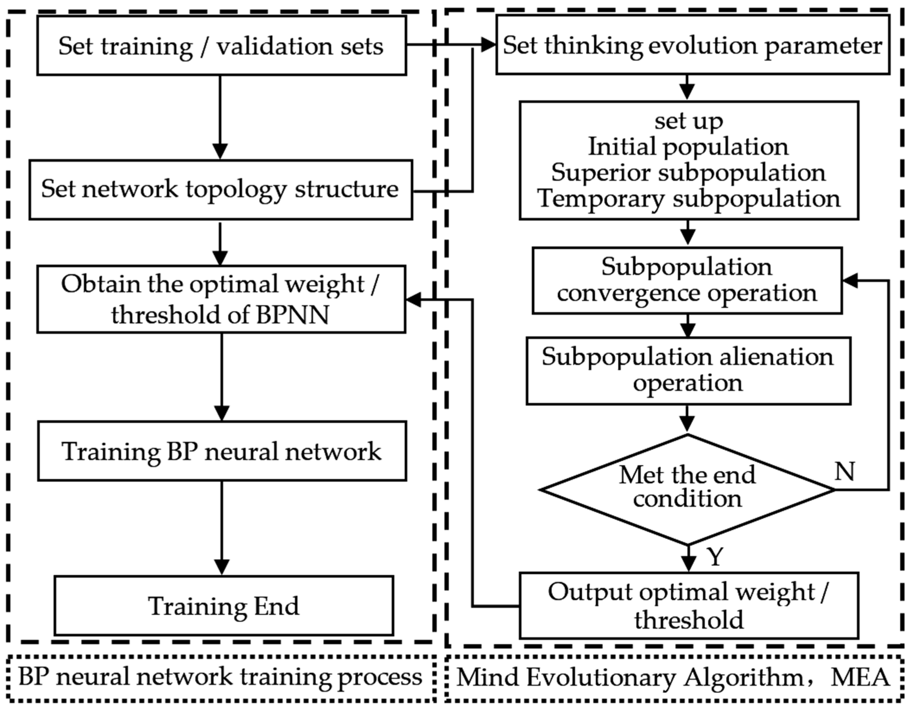
2.3.2. Optimization of BP (Back Propagation) Neural Network Based on Mind Evolution Algorithm (MEA-BPNN)

BP (back propagation) neural network was proposed by Rnmelhart and Hinton in the mid-1980s as a multi-layer feedforward neural network information processing system that simulates human brain function. The two key points in the BP neural network algorithm are the initial weights and thresholds of the network, which play a decisive role in the computational speed and prediction accuracy of the model. Knowing how to quickly and accurately determine the appropriate weights and thresholds is the most critical issue in BP neural network inversion [40,41]. Evolutionary Computation (EC) can be used to solve complex combinatorial optimization problems, but early evolutionary algorithms have problems such as premature convergence and slow convergence when optimizing BP neural networks. The MEA overcomes the drawback of EC [42] and has significant advantages in finding global optimal solutions. Therefore, this study selected the MEA algorithm to optimize the BP neural network estimation model for soil TN content in order to achieve better prediction results.
The MEA is a new type of algorithm optimized on the basis of genetic algorithm. It simulates the evolutionary process of human thinking, and through operations such as “convergence” and “dissimilation” operators, continuously iterates to minimize the error between predicted values and expected values. Figure 1 shows the design process of a BP neural network based on MEA optimization. The basic idea is to first map the solution space to the encoding space based on the topology of the BP neural network after obtaining soil sample data, that is, each encoding corresponds to an individual; then, select the scoring functions of individuals and populations, and continuously iterate and analyze them using the MEA algorithm; finally output the optimal initial weights and thresholds, and use this to train the BP neural network.

3. Results

3.1. Selected Soil TN Characteristic Bands and Their Modeling Effects

The screening results based on correlation coefficients show that in each fertilization period, the characteristic bands of the same transformation at different stages are different but their positions are similar, and the distance between bands does not exceed 10 nm. The characteristic bands of different transformation forms during the same fertilization period are not entirely the same, with the characteristic band positions of 1/R, LogR, and R being the same as that of R; the characteristic bands of all first-order derivative transformations are located similarly, while the characteristic bands of CR are mainly concentrated around 600–900 nm and 2220 nm. For the entire fertilization period, the characteristic band positions of R and 1/R, LogR, and R are basically consistent, which are all around 666 nm. The characteristic band positions of each first-order derivative and CR have changed, but most of them are concentrated around 562, 808, 1429, 1924, and 2223 nm.
The characteristic band screening results based on SMLR show that there is only one sensitive band for R, 1/R, LogR, and R in each fertilization period, which is consistent with the correlation analysis and is close to the results of the entire fertilization period. The bands are 663 nm, 666 nm, 666 nm, and 664 nm, respectively. The number of characteristic bands selected by the first derivative and CR transformation during each fertilization period ranges from 8 to 12, while the number of characteristic bands selected during the entire fertilization period increases from 1 to a maximum of 15, with a few cross bands between different transformations. This is consistent with the results of the correlation analysis method. At the same time, most of the characteristic bands selected based on SMLR for the entire fertilization period include bands selected by the correlation coefficient method or their nearby position bands, but all first-order derivatives and CR transformations have not been selected into the 666 nm band. Based on the screening results of various transformation forms, the bands 562 nm, 706 nm, 808 nm, 1933 nm, and 2345 nm are significantly affected by soil TN content.

3.1.1. Modeling Analysis Based on Univariate Regression

Using the selected characteristic bands as independent variables, univariate regression analysis on soil TN for each fertilization period, including univariate linear, polynomial, and exponential function regression was performed. The results are shown in Table 2. It can be seen that although the univariate regression model based on a single characteristic band is simple and convenient, the overall accuracy is relatively low. Except for the postpartum period (with a maximum R2 of 0.479), the accuracy R2 of the models for other fertilization periods is lower than 0.3, indicating poor modeling performance.
In the same fertilization period, from the perspective of fitting equations, regardless of the transformation form, for univariate regression analysis, the fitting effect of the third-order polynomial model is better than other univariate linear models and exponential models, and the modeling accuracy is slightly higher. From the perspective of spectral transformation forms, the model established based on R has slightly higher accuracy, followed by LogR and 1/R. Among all the univariate regression models, the third-order polynomial model with R is the best for all four fertilization periods. The young fruit stage corresponds to the 663 nm wavelength band, and the modeling determination coefficient R2 = 0.19; the swelling period corresponds to the 666 nm wavelength band, and R2 = 0.264; the quality period corresponds to the 666 nm wavelength band, and R2 = 0.246; and the postpartum period corresponds to the 664 nm wavelength band, with R2 = 0.479. However, overall, compared with R, the accuracy difference between univariate regression models based on 1/R, LogR, and R is very small, and all of them are relatively low. The results indicate that all three transformations have little significance in extracting effective information from soil spectra. Therefore, in the subsequent research on spectral estimation of soil TN content, univariate linear regression analysis may not be necessary.

3.1.2. Modeling Analysis Based on Multiple Regression

  • Modeling effect of characteristic bands based on correlation analysis screening
Based on the correlation coefficient method, the characteristic bands of R and its eight transformations were screened, and multiple sensitive bands could be selected. Therefore, the MLR method was used for modeling and fitting analysis. The results are shown in Table 3. The coefficient of determination R2 of each model is above 0.7. Among them, ( R )′ has the best fitting effect in the young and swollen fruit stages; the model determination coefficient R2 and root mean square error RMSE are 0.74, 0.75, and 0.0047, respectively, in which R2 are 0.55 and 0.49 higher than the univariate regression. CR has the best fitting effect during the quality period, where R2 = 0.78, RMSE = 0.0038, and R2 has a maximum increase of 0.53; (LogR)′ has the best fitting effect during the postpartum period, with R2 = 0.77, RMSE = 0.0039, and R2 increasing by a maximum of 0.37.
Using data from the 40 sampling points in the validation area for each fertilization period, the four selected models with acceptable accuracy were tested. The validation accuracy was evaluated using two indicators: R2 and RMSE, and a 1:1 histogram was created (Figure 2).
It can be seen that, except for the fruit swelling period (R2 = 0.803) and the postpartum period (R2 = 0.779), the validation accuracy of the other period models is less than 0.75.
2.
Modeling effect of characteristic bands based on SMLR screening
Using the characteristic bands screened based on SMLR, MLR fitting was performed on the soil TN content for each fertilization period. The results are shown in Table 4.
From Table 4, it can be seen that based on the principle of maximum R2, models with better soil TN estimation for each fertilization period were selected. Among them, the optimal models for each fertilization period are the MLR models based on CR transformation, with R2 reaching 0.82, 0.84, 0.85, and 0.82, and RMSE being 0.0039, 0.0037, 0.0031, and 0.0034, respectively. Compared with the model established based on correlation analysis screening method, the modeling accuracy increased by 0.095, 0.099, 0.067, and 0.068, respectively, and the RMSE decreased by about 0.001. Secondly, the MLR model based on (LogR)′ performed well, with R2 of 0.81, 0.81, 0.80, and 0.80, and RMSE of 0.0040, 0.0041, 0.0036, and 0.0036, respectively. The maximum variance inflation factor (Max VIF) of all the selected model variables above is less than 10, avoiding the influence of multicollinearity of model variables. To further test the stability and reliability of the model prediction, the four selected models were tested using data from 40 sampling points in the validation area during each fertilization period, and a 1:1 histogram was created (Figure 3). As shown in the figure, except for the quality period (R2 = 0.702), the modeling accuracy of the other three models is higher than 0.8, indicating good validation results.

3.1.3. Modeling and Analysis Based on MEA-BPNN

The characteristic bands selected through the correlation coefficient method and SMLR analysis in R and its various transformation forms were used as input spectra, and the MEA-BPNN was used for modeling. The results are shown in Table 5.
Similar to the MLR method, the model based on SMLR method for screening variables has better performance, with modeling accuracy of over 0.8 except for the young fruit stage (R)′ (R2 = 0.78). Based on the performance of the models in the comprehensive modeling and validation sets, the selected models for each period are all MEA-BPNN models based on CR, with R2 of 0.87, 0.86, 0.86, and 0.88, and RMSE of 0.0043, 0.0033, 0.0043, and 0.0038, respectively. Compared with the model established by MLR method, the accuracy increased by 0.054, 0.021, 0.012, and 0.058, respectively, and the validation accuracy is 0.87, 0.89, 0.84, and 0.87, respectively. In summary, it can be seen that the SMLR method is more effective in screening sensitive bands, and this method will be used for characteristic band screening in future research.

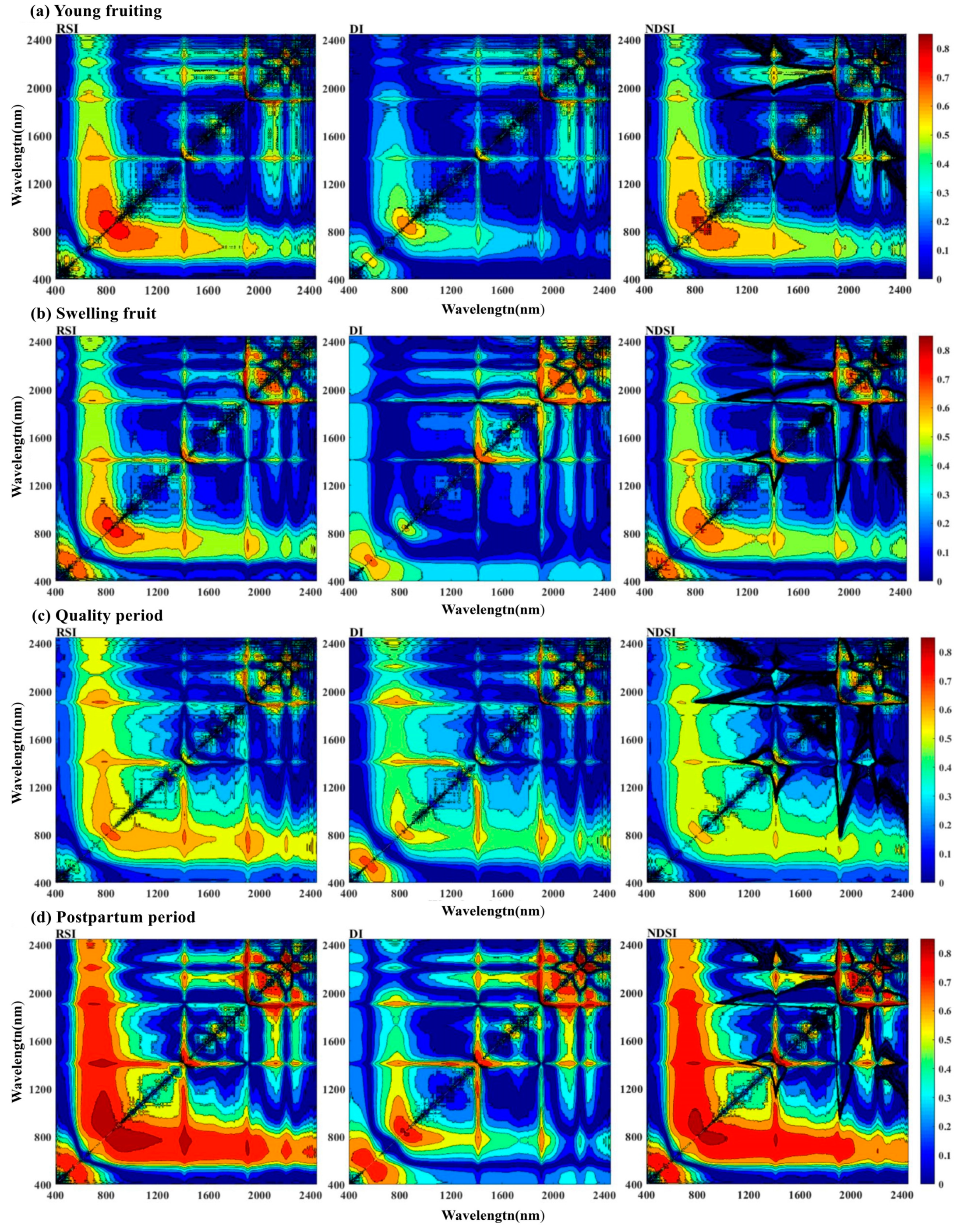
3.2. SCI Screening Results

3.2.1. Independent Soil SCIs for Each Fertilization Period

Figure 4 shows the Isoline map of the correlation coefficient between soil SCI and TN content during each fertilization period. It can be seen that the form of contour maps for each fertilization period is not significantly different, with only slight differences in correlation size. Among them, RSI is the most stable, and the sensitive areas of soil TN are the same in the four fertilization periods, all located in the range of 800–900 nm, 1900–1950 nm, and 2200–2300 nm bands. Under DI and NDSI, the sensitive regions of soil TN during the four fertilization periods are all located in the range of 1900–1950 nm and 2200–2300 nm bands. However, the correlation coefficient of soil TN varies over time in the wavelength range of 800–900 nm, and the quality period performance is poor. The absolute value of the correlation coefficient R is less than 0.6. Therefore, this region will not be considered in the subsequent screening of sensitive differences and normalized spectral indices.
To avoid the multicollinearity effect between variables caused by close band distance, an SCI band combination with the highest correlation was selected for each fertilization period in different sensitive areas of the spectral index (Table 6). It can be seen that the combination bands of each SCI are not within the screening range of the spectral characteristic bands mentioned above, so calculating spectral indices based solely on characteristic bands cannot fully explore spectral information.
The combination bands of various soil spectral characteristic indices during each fertilization period have little interval, and the sensitive areas are mainly concentrated in the range of 800–900 nm, 1900–1950 nm, and 2200–2300 nm bands. Among them, the correlation between characteristic parameters is higher in the range of 1900–1950 nm. To reduce data redundancy, only these three regions are used as screening areas for spectral characteristic parameters in conducting large-scale data analysis during the entire fertilization period.

3.2.2. Comprehensive Soil SCI during the Entire Fertilization Period

Based on the sensitive areas of SCI during each fertilization period, the screening of comprehensive soil SCI for the entire fertilization period of the orchard was conducted. A band combination with the highest correlation was selected in different sensitive areas of the spectral indices. The results are shown in Table 7. Correlation coefficient contour analysis between SCI and TN during the entire fertilization period was performed (Figure 5). It can be seen that 1904 nm and 1949 nm perform well in both RSI and DI, consistent with the results of each period, indicating that this band range has advantages in SCI screening.

3.3. Estimation Model Based on SCI and Characteristic Band Combination

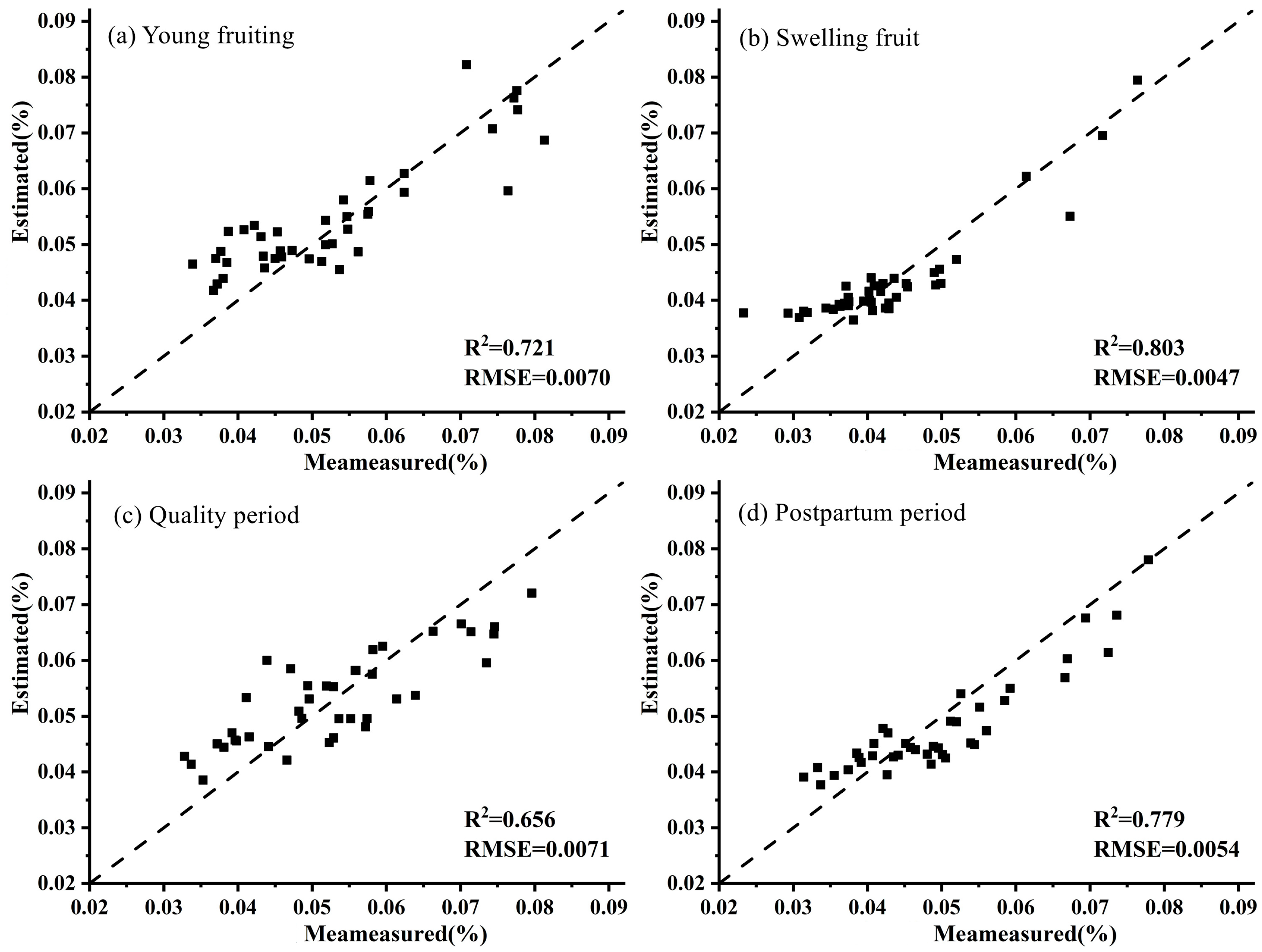
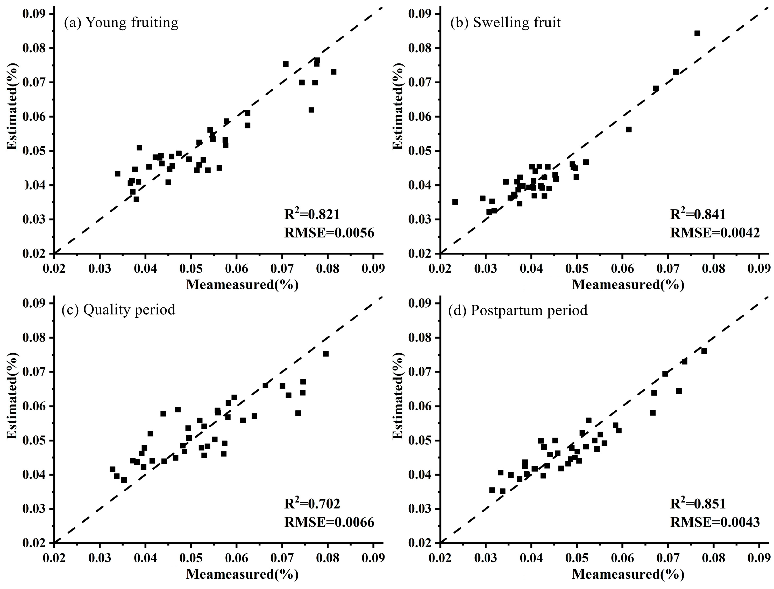
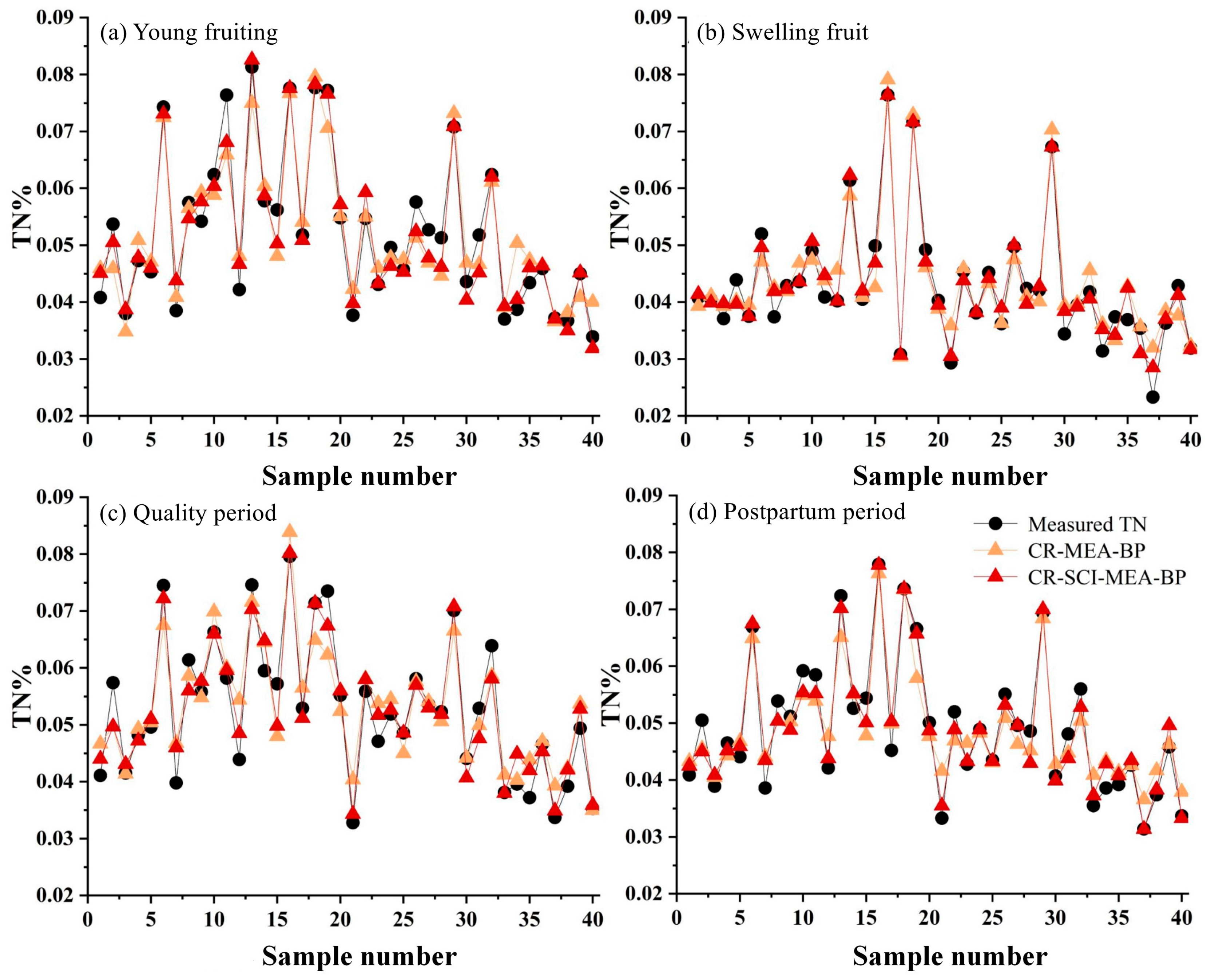
3.3.1. Independent Estimation Models for Each Fertilization Period

The seven SCIs (three RSIs, three DIs, and two NDSIs) were used together with the SMLR selected characteristic bands as independent variables, and the soil TN content in each period was used as the training target. MLR and MEA-BPNN were used for modeling, respectively. The results are shown in Table 8.
Overall, regardless of the modeling method, the addition of SCI has improved the modeling accuracy. Among them, the two models constructed based on CR transformation have slightly higher modeling and validation accuracy than the other transformation methods. Therefore, it can be proven that this transformation form has advantages in spectral processing. Compared with the two modeling methods, the MEA-BPNN model still maintains its modeling advantages, with better performance in R2 and RMSE than the MLR model, and some models have modeling accuracy greater than 0.9.
Based on the comprehensive performance of each fertilization period model, the optimal models were selected based on the CR-MEA-BP method, with R2 of 0.94, 0.95, 0.92, and 0.94, and RMSE of 0.0032, 0.0024, 0.0035, and 0.0027, respectively. Compared with MLR, the modeling accuracy increased by 0.068, 0.089, 0.054, and 0.066, respectively, and the validation accuracy was 0.92, 0.93, 0.91, and 0.93, respectively.
In each fertilization period, the optimized model with SCI correction and its original model were used to predict soil TN, and the prediction curves of SCI-MEA-BPNN and MEA-BPNN were obtained for each fertilization period (Figure 6). It can be seen that the model prediction curve with the addition of SCI is more consistent with the measured value curve, and the prediction effect is better. The overall trend of the MEA-BP predicted value curve without SCI input is consistent with the measured value curve, but the degree of conformity is slightly poor. It has a good prediction effect on samples with gentle changes, and a large prediction error at extreme points. This demonstrates the positive effect of adding SCI to the construction of soil TN content prediction models.

3.3.2. Comprehensive Estimation Model for the Entire Fertilization Period

Based on the soil TN content, original spectral reflectance, and various transformation forms of 400 sample data from 100 sampling points during four fertilization periods in the modeling area, the SMLR method was used to extract characteristic bands, and together with the seven extracted SCIs, a unified soil TN estimation model for the orchard’s entire fertilization period was constructed. And a total of 160 sample data from 40 sampling points during four fertilization periods in the validation area were used for validation.
The MLR and MEA-BPNN modeling results of the soil TN content based on the original soil spectrum and its first derivative transformation during the entire fertilization period of the orchard are shown in Table 9.
It can be seen that the addition of SCI has less advantages in the estimation model of the entire fertilization period than in the small sample size estimation model of each period. The modeling accuracy of each model based on the first derivative transformation and the CR transformation after adding the index is relatively small, and the validation accuracy is not significantly different from before. However, the prediction performance of the model based on the original spectral reflectance is significantly improved after adding an index. This indicates that the SCI has a better correction effect on linear models with fewer variables and lower modeling accuracy.
Unlike the results of soil TN estimation models for different fertilization periods, the advantage of the CR method in the study of soil TN content MLR models for the entire fertilization period is not significant, while the modeling effect of ( R )′ and (LogR)′ is better. According to the size of R2, it can be seen that the addition of SCI has a more positive effect on the MEA-BPNN. For instance, The accuracy of modeling and validation increases more compared to MLR models. The performance of each spectral transformation is basically consistent with the results of soil TN content estimation modeling in each fertilization period. The CR-SCI-MEA-BP model has the best prediction performance, with R2 and RMSE of 0.899, 0.0038, and 0.89, 0.0041, respectively, in the modeling and validation sets.

4. Discussion

In this article, the extraction method of hyperspectral parameters for TN content in apple orchard soil was explored and its estimation model was optimized. The results show that SMLR is effective and has significant advantages in extracting hyperspectral characteristic bands of soil TN content; moreover, the combination of SCI and characteristic bands, and the use of the MEA-BPNN method for independent and comprehensive estimation of soil TN content during each fertilization period and entire fertilization period, have the best modeling effect.

4.1. Collection and Preprocessing of Hyperspectral Data on TN in Orchard Soil

The soil spectrum is the result of the joint action of various components in the soil, and the relationship between soil spectral reflectance and various nutrients in the soil is extremely complex [9,11]. Most apple orchards are located in mountainous and hilly areas, which are affected by factors such as geography, climate, and soil texture. The soil nitrogen content is low, the spectral signal is weak, and it is easy to be disturbed or masked, making it difficult to obtain effective spectral information [31]. For this reason, previous studies have mostly collected spectra of ground and sieved samples under strictly controlled indoor conditions, resulting in a higher modeling accuracy of the measured spectra. This approach is far from orchards and extends the estimation time, which is not suitable for the real-time management needs of modern orchards [29,32]. However, field measurements are greatly influenced by the weather and surrounding environmental conditions, which can lead to the inability to guarantee the accuracy of the model [43]. Especially, modern orchards generally adopt ecological planting methods such as intercropping or grass planting [44], where light is often obstructed by fruit trees and other plants, and it is not suitable to directly collect soil spectra. Therefore, this article adopts the method of manually controlling the surrounding outdoor environment and using natural sunlight as a light source to collect spectral data. In this way, spectral collection has taken a step closer from indoors to orchard fields, providing a beneficial exploration for future spectral collection in complex orchard environments. At the same time, in order to assist with orchard fertilization management, soil samples were collected 10 days before the fertilization day. This is beneficial for understanding the soil nutrient situation after the previous fertilization period and providing guidance for the next fertilization period.
Performing (1/R), (LogR), ( R ), and their first derivative transformations on the original spectral reflectance R can further reduce the noise effects caused by non-target factors such as lighting conditions, soil particle size, and air moisture in spectral measurements; highlight effective information in the spectrum; improve the sensitivity of characteristic bands [28]; and explore the optimal spectral transformation form [45]. CR, also known as envelope division, can effectively enhance the spectral characteristics of the region of interest [46,47,48]. The results of this study also demonstrated that CR is beneficial for extracting characteristic spectral information and effectively improving the response ability of spectral data to soil TN. Through modeling and prediction performance analysis, it was found that various first-order derivative transformations and CR transformations of reflectance can improve the prediction accuracy of the corresponding fertilization period estimation model, which has positive significance for the spectral estimation research of soil TN. However, the prediction performance of the 1/R, LogR, and R models is not ideal. In addition, the characteristic bands selected by various transformations are different, and the estimation models for soil TN content during different fertilization periods also differ.

4.2. Extraction of Characteristic Bands and Selection of SCI

Due to the varying degrees of influence of different spectral bands on the soil TN content, in order to establish the optimal model, it is necessary to filter out the bands that have little impact on the soil TN content and leave behind the most suitable characteristic bands for modeling [11,43,45]. This article compares the screening effects of the correlation coefficient method and SMLR based on R and its eight transformations.
The results indicate that the correlation coefficient method can determine the characteristic band range of soil TN to some extent, providing a basis for the selection of characteristic bands. Choosing the band at the extreme point of the correlation coefficient as the input variable to construct the model has the advantages of simplicity, clarity, and strong operability. However, the selection of bands located at the extreme points of the correlation coefficient is subjective and cannot estimate the interrelationships between bands at the extreme points, thus ultimately failing to achieve ideal model prediction results [49].
SMLR is a good variable screening method, and a large number of studies have shown that all independent variables retained after stepwise regression analysis have a significant impact on the dependent variable [26,50]. In SMLR, this article refers to the correlation between variables and the variance inflation factor (VIF), and selects variables included in the equation that pass the 0.05 significance level test and have a maximum variance inflation factor of no more than 10 as the characteristic bands of soil TN [51]. In this way, the problem of multicollinearity between bands that are closely spaced within the same regression equation is avoided, and the modeling effect is improved. The results of this article indicate that compared with the correlation coefficient method, using the SMLR method to screen characteristic bands can avoid collinearity issues caused by band spacing while considering spectral characteristic information [35]. Although the selected bands are not located at the extreme points of the correlation coefficient, the predictive performance and stability of the model are slightly better than the previous screening method. It should be noted that there is a significant difference between the characteristic bands selected based on SMLR and the corresponding correlation coefficient characteristic bands during each fertilization period. Except for the characteristic bands transformed by the first derivative of the original reflectance, the positions of the other transformed characteristic bands are mostly far apart. It is difficult to screen the same spectral band for multiple spectral transformations during different fertilization periods. Therefore, this paper established an estimation model and validated it for evaluation in order to select a more suitable extraction method for characteristic bands. Compared with the correlation coefficient method, the model established based on the characteristic bands selected by the SMLR method can achieve higher modeling accuracy and smaller RMSE under the same spectral transformation. Moreover, it is easier to select models with a maximum variance inflation factor of less than 10, thus avoiding the influence of multicollinearity of model variables.
It can be seen that regardless of which characteristic band selection method is used, the modeling effect of the MEA-BPNN is superior to the MLR method, and the modeling accuracy has been improved, but the RMSE of some models has only slightly improved. The SMLR method performs better in screening sensitive bands and exhibits greater advantages. It has good practicality in constructing and predicting both linear and nonlinear models. Therefore, in the study of spectral estimation of soil TN content during the entire fertilization period, this article did not further construct a sensitive band model based on correlation analysis. Instead, the significant bands selected by SMLR and the SCI selected were mainly used as input spectra for the study.
In terms of SCI, research on models in different periods has found that the addition of SCI has a positive effect on the prediction accuracy of various types of models [36]. Overall, the addition of SCI can improve the prediction accuracy of the model, reduce RMSE, and make the estimation model more stable [37]. Therefore, this article determines the strategy for modeling using the combination of SCI and characteristic bands.

4.3. About Modeling Methods

Regression analysis is a common statistical analysis method used to determine the quantitative relationship between two or more variables [52] and is widely used in the quantitative estimation of soil nutrients [53].
The results of this article show that the modeling effect of univariate regression is not satisfactory. This indicates that even if a certain band has a high correlation with soil TN, it cannot cover all the effective information. Relying solely on a single band for the spectral estimation of soil TN in apple orchards is not ideal. However, simple univariate regression models can still be used to evaluate the significance and value of various transformations in extracting effective spectral information.
The use of MLR for the quantitative estimation of soil TN content is simple. Compared to univariate regression models, the MLR models have higher modeling accuracy [50]. When there is a strong linear relationship between soil TN and characteristic bands, the modeling effect is better, but the selection of characteristic bands requires higher requirements. There should be no strong collinearity between bands, and the number of bands should not exceed the number of modeling samples. This can be solved by the SMLR filtering of characteristic bands [33]. Overall, the linear regression model is relatively simple, computationally small, and has strong operability. The predictive effect of the model is acceptable, and it can achieve a rough prediction of soil TN content in the orchard.
The BP neural network can handle nonlinear relationships between variables well and has great advantages in the spectral prediction of soil physical and chemical properties [54,55,56]. The MEA overcomes the shortcomings of EC such as premature convergence and slow convergence speed [42], solves complex combinatorial optimization problems, and facilitates the search for global optimal solutions, ultimately minimizing the error between the predicted and expected values. The modeling results of this article indicate that the model based on MEA-BPNN has higher accuracy and stability and can more accurately estimate soil TN content. The disadvantage is that the model is relatively complex and computationally intensive. This can utilize computers to achieve automated calculations and improve the practicality of the model. Among the estimation models for each fertilization period and the entire fertilization period, the model based on CR-SCI-MEA-BPNN has the best prediction performance. It should be pointed out that there are currently not many studies on the hyperspectral inversion of total nitrogen in apple orchard soil, especially for different fertilization periods, which have not been reported yet [25,26,30]. Our research was conducted in a relatively small apple orchard in Shandong Province; due to differences in natural conditions and management practices among orchards in different regions, this may limit the generalizability of research results to other regions or orchards with different soil and climate conditions. Therefore, in the future, research on the application of orchards in different regions, climates, and soil conditions should be carried out.

5. Conclusions

This article collected the soil spectral reflectance of apple orchards during different fertilization periods. The original spectral reflectance (R) and its eight transformations, including (1/R), (LogR), ( R ) and their first derivative transformation, as well as CR, were used to extract the characteristic bands of soil TN using the correlation coefficient method and SMLR. The best characteristic band extraction method was selected by comparing and analyzing the modeling effects of linear regression and the MEA-BPNN method. Band by band analysis techniques and correlation analysis methods were used to select the SCI suitable for soil TN. Based on the selected SCI and characteristic band combinations, MLR and MEA-BPNN were used to construct and optimize independent and comprehensive soil TN content estimation models for each fertilization period and the entire fertilization period, respectively.
The results indicate that SMLR is effective and has significant advantages in extracting hyperspectral characteristic bands of soil TN content. Compared with the correlation coefficient method, under the same spectral transformation, the model based on SMLR filtering for characteristic bands can achieve a higher modeling accuracy and smaller RMSE. Moreover, it is easier to select models with a maximum VIF of less than 10 to avoid the influence of multicollinearity of model variables.
The sensitive areas of soil TN content in the SCI do not undergo significant changes due to different fertilization periods. Among them, the RSIs are in the range of 800–900 nm, 1900–1950 nm, and 2200–2300 nm, while the sensitive areas of the DI and NDSI are in the range of 1900–1950 nm and 2200–2300 nm.
The addition of SCI and characteristic band combination significantly improves the prediction accuracy of soil TN model. The independent and comprehensive soil TN content estimation models for each fertilization period based on MEA-BPNN can achieve stable and accurate soil TN estimation. Among the estimation models for each fertilization period and the entire fertilization period, the model based on CR-SCI-MEA-BPNN has the best prediction performance.

Author Contributions

Conceptualization, W.W. and Z.G.; methodology, W.W. and Z.G.; software, W.W., Z.G. and R.L.; validation, Z.G. and W.W.; formal analysis, Z.G. and W.W.; investigation, W.W., H.W. and R.L.; resources, W.W.; data curation, W.W., R.L. and Z.G.; writing—original draft preparation, W.W. and Z.G.; writing—review and editing, Z.G. and W.W.; visualization, W.W. and Z.G.; supervision, H.W.; project administration, R.L. and H.W.; funding acquisition, W.W. and R.L. All authors have read and agreed to the published version of the manuscript.

Funding

This research was funded by the Key R&D Program Project in Shandong Province (2018CXGC0209), and Natural Science Foundation of Shandong Province (ZR2021MD018).

Data Availability Statement

Data are contained within the article.

Acknowledgments

We thank the anonymous reviewers for their valuable comments and suggestions.

Conflicts of Interest

Wenqian Wang was employed by the company Shandong Yuanhong Survey Planning and Design Co., Ltd. The remaining authors declare that the research was conducted in the absence of any commercial or financial relationships that could be construed as a potential conflict of interest.

References

  1. Wang, Y. China’s apple production steadily ranks first in the world. Farmers Daily, 18 November 2023. [Google Scholar]
  2. Peng, F.T.; Jiang, Y.M.; Gu, M.R.; Shu, H.R. Advances in research on nitrogen nutrition of deciduous fruit crops. J. Fruit Sci. 2003, 20, 54–58. [Google Scholar]
  3. Gao, Y.M.; Tong, Y.A.; Lu, Y.L.; Wang, X.Y. Effects of soil available nutrients and long-term fertilization on yield of Fuji apple orchard of Weibei area in Shaanxi, China. Acta Hortic. Sin. 2013, 40, 613–622. [Google Scholar] [CrossRef]
  4. Zhang, Y.Z.; Cheng, C.G.; Zhao, D.Y.; Zhou, J.T.; Chen, Y.H.; Zhang, H.T.; Xie, B. Effects of nitrogen application levels on fruit Ca forms and quality of ‘Fuji’ apples. J. Plant Nutr. Fert. 2021, 27, 87–96. [Google Scholar]
  5. Li, Y.; Xiao, J.; Yan, Y.; Liu, W.; Cui, P.; Xu, C.; Nan, L.; Liu, X. Multivariate analysis and optimization of the relationship between soil nutrients and berry quality of vitis vinifera cv. cabernet franc vineyards in the eastern foothills of the Helan mountains, China. Horticulturae 2024, 10, 61. [Google Scholar] [CrossRef]
  6. Raese, J.T.; Drake, S.R.; Curry, E.A. Nitrogen fertilizer influences fruit quality, soil nutrients and cover crops, leaf color and nitrogen content, biennial bearing and cold hardiness of ‘Golden Delicious’. J. Plant Nutr. 2007, 30, 1585–1604. [Google Scholar] [CrossRef]
  7. Deng, J.; Feng, X.Q.; Wang, D.Y.; Lu, J.; Chong, H.T.; Shang, C.; Liu, K.; Huang, L.Y.; Tian, X.H.; Zhang, Y.B. Root morphological traits and distribution in direct-seeded rice under dense planting with reduced nitrogen. PLoS ONE 2020, 15, e0238362. [Google Scholar] [CrossRef]
  8. Zhang, J.H. Nitrgen imbalance in apple trees and its application in science and technology. Hortic. Seed. 2016, 35, 56–59. [Google Scholar] [CrossRef]
  9. Bai, Z.J.; Peng, J.; Luo, D.F.; Cai, H.H.; Ji, W.J.; Shi, Z.; Liu, W.Y.; Yin, C.Y. A mid-infrared spectral inversion model for total nitrogen content of farmland soil in southern Xinjiang. Spectrosc. Spect. Anal. 2022, 42, 2768–2773. [Google Scholar]
  10. Zhang, G.B.; Li, X.C.; Qi, F.Y.; Wu, B.; Cheng, S.H. Grey cluster estimating model of soil organic matter content based on hyperspectral data. J. Grey Syst. UK 2014, 26, 28–37. [Google Scholar]
  11. Peng, J.; Zhang, Y.Z.; Zhou, Q.; Pang, X.A.; Wu, W.M. The progress on the relationship physics-chemistry properties with spectrum characteristic of the soil. Chin. J. Soil. Sci. 2009, 40, 1204–1208. [Google Scholar] [CrossRef]
  12. Guo, Y.; Guo, Z.X.; Liu, J.; Yuan, Y.Z.; Sun, H.; Chai, M.; Bi, R.T. Hyperspectral inversion of paddy soil iron oxide in typical subtropical area with Pearl River Delta, China as illustration. J. Appl. Ecol. 2017, 28, 3675–3683. [Google Scholar]
  13. Vasques, G.M.; Grunwald, S.; Harris, W.G. Spectroscopic models of soil organic carbon in Florida. USA. J. Environ. Qual. 2010, 9, 23–934. [Google Scholar] [CrossRef]
  14. Liu, J.B.; Han, J.C.; Zhang, Y.; Wang, H.Y.; Kong, H.; Shi, L. Prediction of soil organic carbon with different parent materials development using visible-near infrared spectroscopy. Spectrochim. Acta A 2018, 204, 33–39. [Google Scholar] [CrossRef]
  15. Liao, Q.H.; Gu, X.H.; Li, C.J.; Chen, L.P.; Huang, W.J.; Du, S.Z.; Fu, Y.Y.; Wang, J.H. Estimation of fluvo-aquic soil organic matter content from hyperspectral reflectance based on continuous wavelet transformation. Trans. CSAE 2012, 28, 132–139. [Google Scholar]
  16. Lin, L.X.; Wang, Y.J.; Teng, J.Y.; Wang, X.C. Hyperspectral analysis of soil organic matter in coal mining regions using wavelets, correlations, and partial least squares regression. Environ. Monit. Assess 2016, 188, 1–11. [Google Scholar] [CrossRef]
  17. Divya, Y.; Gopinathan, P. Soil water content measurement using hyper-spectral remote sensing techniques—A case study from north-western part of Tamil Nadu, India. Remote Sens. Appl. Soc. Environ. 2019, 14, 1–7. [Google Scholar] [CrossRef]
  18. Yang, H.; Kuang, B.; Mouazen, A.M. Quantitative analysis of soil nitrogen and carbon at a farm scale using visible and Near Infrared spectroscopy coupled with wavelength reduction. Eur. J. Soil. Sci. 2012, 63, 410–420. [Google Scholar] [CrossRef]
  19. Xie, H.T.; Yang, X.M.; Drury, C.F.; Yang, J.Y.; Zhang, X.D. Predicting soil organic carbon and total nitrogen using Mid-and Near-infrared spectra for brookston clay loam soil in sourth-western Ontario, Canada. Can. J. Soil. Sci. 2011, 91, 53–63. [Google Scholar] [CrossRef]
  20. Zhang, J.J.; Tian, Y.C.; Yao, X.; Cao, W.X.; Ma, X.M.; Zhu, Y. Estimating model of soil total nitrogen content based on near-infrared spectroscopy analysis. Trans. CSAE 2012, 28, 183–188. [Google Scholar]
  21. Liu, X.Y.; Wang, L.; Chang, Q.R.; Wang, X.X.; Shang, Y. Prediction of total nitrogen and alkali hydrolysable nitrogen content in loess using hyperspectral data based on correlation analysis and partial least squares regression. Chin. J. Appl. Ecol. 2015, 26, 2107–2114. [Google Scholar]
  22. Li, Y.; Wang, R.H.; Guan, Y.L.; Jiang, H.L.; Wu, X.Q.; Peng, Q. Prediction analysis of soil total nitrogen content based on hyperspectral. Remote Sens. Technol. Appl. 2017, 32, 173–179. [Google Scholar]
  23. Jia, S.Y.; Li, H.Y.; Wang, Y.J.; Tong, R.Y.; Li, Q. Hyperspectral Imaging Analysis for the classification of soil types and the determination of soil total nitrogen. Sensors 2017, 17, 2252. [Google Scholar] [CrossRef]
  24. Niu, Z.; Shi, L.; Qiao, H.; Xu, X.; Wang, W.; Ma, X.; Zhang, J. Construction of a hyperspectral estimation model for total nitrogen content in Shajiang black soil. J. Plant Nutr. Soil. Sci. 2023, 186, 196–208. [Google Scholar] [CrossRef]
  25. Li, Z.; Zhang, G.C.; An, X.H.; Li, M.; Li, E.M.; Cheng, G.G. Estimation for available nitrogen content of apple orchard soil by near infrared spectroscopy and partial least squares regression. North. Hortic. 2018, 3, 113–119. [Google Scholar]
  26. Yu, X.; Liu, Q.; Wang, Y.B.; Liu, X.Y.; Liu, X. Evaluation of MLSR and PLSR for estimating soil element contents using visible/near-infrared spectroscopy in apple orchards on the Jiaodong peninsula. Catena 2016, 137, 340–349. [Google Scholar] [CrossRef]
  27. Liu, Y.D.; Xiong, S.S.; Chen, D.B. Estimation of the TN and SOM contents in soil from GAN NAN navel orange plant area by NIR diffuse spectroscopy. Spectrosc. Spect. Anal. 2013, 33, 2679–2682. [Google Scholar]
  28. Tang, R.N.; Li, X.W.; Li, C.; Jiang, K.X.; Hu, W.F.; Wu, J.J. Estimation of total nitrogen content in rubber plantation soil based on hyperspectral and fractional order derivative. Electronics 2022, 11, 1956. [Google Scholar] [CrossRef]
  29. Liu, T.L.; Zhu, X.C.; Bai, X.Y.; Peng, Y.F.; Li, M.X.; Tian, Z.Y.; Jiang, Y.M.; Yang, G.J. Hyperspectral estimation model construction and accuracy comparison of soil organic matter content. Smart Agric. 2020, 2, 129–138. [Google Scholar]
  30. Liu, Z.M.; Li, X.Q.; Chen, G.L.; Ding, H.P.; Xu, M.G.; Yang, C.X. Inversion of soil total nitrogen content in Yunnan Rubber plantation based on hyperspectral. Trop. Agric. Sci. Technol. 2023, 46, 35–41. [Google Scholar]
  31. Wang, W.Q.; Gao, M.X.; Lang, K.; Wang, J.F. Hyperspectral estimation of total nitrogen in apple orchard soil based on wavelet transform. J. Shandong Agric. Univ. 2021, 52, 845–852. [Google Scholar] [CrossRef]
  32. Chen, H.Y.; Zhao, G.X.; Li, X.C.; Zhu, X.C.; Sui, L.; Wang, Y.J. Hyper-spectral estimation of soil organic matter content based on wavelet transformation. Chin. J. Appl. Ecol. 2011, 22, 2935–2942. [Google Scholar]
  33. Wang, L.W.; Wei, Y.X. Estimating the total nitrogen and total phosphorus content of wetland soils using hyperspectral models. Acta Ecol. Sin. 2016, 36, 5116–5125. [Google Scholar]
  34. Qiu, H.; Chen, H.Y.; Xing, S.H.; Zhang, L.M.; Dong, X.Y. Soil organic matter estimation models based on Hyperion data. J. Fujian Agric. For. Univ. 2017, 46, 460–467. [Google Scholar]
  35. Li, X.J.; Wang, M.L.; Zhao, M.; Shi, Y.H.; Gao, Q. Vineyard drought monitoring model based on multiple stepwise regression analysis. Agric. Res. Arid. Areas 2022, 40, 249–254. [Google Scholar]
  36. Nie, X.J.; Zhao, X.H.; Ammara, G.; Hong, W.W.; Zhang, H.B. Inversion of coal-derived carbon content in mine soils based on hyperspectral index and machine learning. J. Chin. Coal Soc. 2023, 48, 2869–2880. [Google Scholar]
  37. Li, C.; Zhang, G.W.; Zhou, Z.G.; Zhao, W.Q.; Meng, Y.L.; Chen, B.L.; Wang, Y.H. Hyperspectral parameters and prediction model of soil moisture in coastal saline. Chin. J. Appl. Ecol. 2016, 27, 525–531. [Google Scholar]
  38. Liu, J.F.; Zhao, Z.Y.; Li, C.Y.; Gao, Y.; Zhao, X.; Jiang, W.G.; Gong, Z. Estimation of apple tree canopy SPAD based on UAV multispectral remote sensing. J. Drain. Irrig. Mach. Eng. 2024. Available online: https://link.cnki.net/urlid/32.1814.TH.20240115.1641.004 (accessed on 16 February 2024).
  39. Leng, J.F.; Gao, X.; Zhu, J.P. The application of multiple linear regression statistical prediction models Statistics and decision-making. Stat. Decis. 2016, 7, 82–85. [Google Scholar]
  40. Wen, X. Applying MATLAB to Implement Neural Networks; National Defense Industry Press: Beijing, China, 2015; p. 95. [Google Scholar]
  41. Liu, B.Y.; Zhang, J.H.; Geng, S.C.; Tao, J.J.; Feng, Y. Estimation of N2o emission flus from heterotrophic nitrification process in global forest soils based on BP neural network model. Chin. J. Ecol. 2022, 41, 209–217. [Google Scholar] [CrossRef]
  42. Sun, C.Y.; Xie, K.M.; Cheng, M.Q. Mind-evolution-based machine learning framework and new development. J. Taiyuan Univ. Technol. 1999, 43, 3–7. [Google Scholar]
  43. Liu, H.J.; Zhang, X.L.; Zheng, S.F.; Tang, N.; Hu, Y.L. Black soil organic matter prediction model based on field hyperspectral reflectance. Spectrosc. Spect. Anal. 2010, 30, 3355–3358. [Google Scholar]
  44. Bai, G.S.; Zou, C.Y.; Du, S.N. Effects of self-sown grass on soil moisture and tree growth in apple orchard on Weibei dry plateau. Trans. CSAE 2018, 34, 151–158. [Google Scholar] [CrossRef]
  45. Shen, Y.; Zhang, X.P.; Yang, X.M.; Liang, A.Z.; Shi, X.H.; Fan, R.Q. Effects of data pretreatment and spectrum bands on near infrared spectroscopy model of soil organic carbon in black soil. ACTA Pedol. Sin. 2010, 47, 1005–1012. [Google Scholar]
  46. Philippe, L.; Baret, F.; Feret, J.B.; José, M.N.; Jean, M. R-M. Estimation of soil clay and calcium carbonate using laboratory, field and airborne hyperspectral measurements. Remote Sens. Environ. 2007, 112, 825–835. [Google Scholar]
  47. Peng, J.; Chi, C.M.; Xiang, H.Y.; Teng, H.F.; Shi, Z. Inversion of soil salt content based on continuum-removal method. ACTA Pedo Sin. 2014, 51, 459–469. [Google Scholar]
  48. Xiang, H.Y.; Liu, W.Y.; Peng, J.; Wang, J.Q.; Chi, C.M.; Niu, J.L. Predicting organic matter content in paddy soil using method of continuum removal in southern Xinjiang, China. Soils 2016, 48, 389–394. [Google Scholar]
  49. Yang, D.H.; Li, Y.Q.; Dao, J.; Wang, J.X. Estimation of soil main nutrient content based on unmanned aerial vehicle multispectral and ground hyperspectral remote sensing. Jiangsu Agri. Sci. 2022, 50, 178–186. [Google Scholar] [CrossRef]
  50. Wei, L.S. Mathematical Statistics; Science Press: Beijing, China, 2024; p. 1. [Google Scholar]
  51. Xu, Y.; Shao, G.C.; Ding, M.M.; Zhang, E.Z.; He, J. Inversion model of soil total nitrogen content based on ridge regression. J. Drain. Irrig. Mach. Eng. 2022, 40, 1159–1166. [Google Scholar]
  52. Ren, H.; Guo, C.L.; Zhao, Z.P.; He, Q.M.; Chen, D.M. Current status of vision and its influencing factors among primary students in Meilan district of Haikou city. Pract. Prev. Med. 2020, 27, 54–56. [Google Scholar]
  53. Xu, Y.M.; Lin, Q.Z.; Huang, X.H.; Shen, Y.; Wang, L. Experimental study on total nitrogen concentration in soil by VNIR reflectance spectrum. Geogr. Geo. Inform. Sci. 2005, 21, 19–22. [Google Scholar]
  54. Lu, Z.H.; Liu, X.Y.; Chang, S.J.; Yang, S.L.; Zhao, W.W.; Yang, Y.; Liu, A.J. Hyperspectral inversion of the surface soil N/P ratio in a grassland mining area based on the BP neural network. Pratac. Sci. 2018, 35, 2127–2136. [Google Scholar]
  55. Zhao, J.H.; Zhang, C.Y.; Min, L.; Li, N.; Wang, Y. Retrieval for soil moisture in farmland using multi-source remote sensing data and feature selection with GA-BP neural network. Trans. CSAE 2021, 37, 112–120. [Google Scholar]
  56. Wang, S.D.; Shi, P.J.; Zhang, H.B.; Wang, X.C. Retrieval of soil total nitrogen content in reclaimed farmland of mining area based on hyperspectral imaging. Chin. J. Ecol. 2019, 38, 294–301. [Google Scholar]
Figure 1. BP (back propagation) neural network (BPNN) flowchart optimized based on Mind Evolutionary Algorithm (MEA).
Horticulturae 10 00358 g001
Figure 2. Comparison of measured and estimated values of soil TN content during different fertilization periods using model based on characteristic bands screened with correlation analysis. (a) young fruiting, (b) swelling fruit, (c) quality period, (d) postpartum period.
Horticulturae 10 00358 g002
Figure 3. Comparison of measured and estimated values of soil TN content during different fertilization periods using model based on characteristic bands screened with stepwise multiple linear regression. (a) young fruiting, (b) swelling fruit, (c) quality period, (d) postpartum period.
Horticulturae 10 00358 g003
Figure 4. Isoline maps of correlation coefficient between soil spectral characteristic index (SCI) and TN content for each fertilization period. (a) young fruiting, (b) swelling fruit, (c) quality period, (d) postpartum period. Note: RSI: ratio spectral index; DI: difference spectral index; NDSI: Normalized difference spectral index. The same below.
Horticulturae 10 00358 g004
Figure 5. Isoline maps of the correlation coefficient between soil spectral characteristic index (SCI) and soil TN content during the entire fertilization period.
Horticulturae 10 00358 g005
Figure 6. Comparison of measured and estimated values of soil TN content in different models during different fertilization periods. (a) young fruiting, (b) swelling fruit, (c) quality period, (d) postpartum period.
Horticulturae 10 00358 g006
Table 1. Descriptive statistical characteristics of soil TN content in each fertilization periods.
Study AreaSample SizeIndexSoil TN Content (%)
Young FruitSwellingQualityPostpartum
Modeling area100Max0.08400.07260.08820.0812
Min0.03530.02540.04060.0307
Mean0.05120.04270.05230.0482
Validation area40Max0.08130.07640.07960.0779
Min0.03390.02330.03280.0290
Mean0.05260.04280.05280.0491
Table 2. Univariate regression analysis of soil original reflectance and its transformation form with soil TN content in each fertilization period.
Sampling PeriodInput SpectrumRegression EquationR2RMSE
Young fruitingx = R663y = −0.2146x + 0.09540.1010.0087
y = −349.8x3 + 228.8x2 − 49.818x + 3.66040.1830.0083
y = 0.1095e3.755x0.0940.0091
x = 1/R663y = 0.0098x + 0.00330.1370.0086
y = 0.0251x3 − 0.3515x2 + 1.6407x − 2.50310.1860.0083
y = 0.022e0.171x0.1040.0090
x = LogR663y = −0.0461x − 0.02170.1070.0087
y = −3.0554x3 − 14.048x2 − 21.523x − 10.9380.1890.0083
y = 0.0142e0.804x0.0990.0089
x = R 663 y = −0.1991x + 0.14160.1040.0087
y = −263.37x3 + 368.04x2 − 171.39x + 26.6460.1900.0083
y = 0.2445e3.477x0.0970.0092
Swelling fruitx = R666y = −0.2376x + 0.09820.2380.0081
y = −34.815x3 + 28.138x2 − 7.6531x + 0.73740.2640.0080
y = 0.1394e5.166x0.2270.0082
x = 1/R666y = 0.013x − 0.01340.2510.0081
y = −0.0004x3 + 0.013x2 − 0.0782x + 0.16820.2640.0080
y = 0.0124e0.282x0.23760.0084
x = LogR666y = −0.0558x − 0.03870.2450.0081
y = −0.1746x3 − 0.5915x2 − 0.6622x − 0.20770.2640.0082
y = 0.0071e1.212x0.2330.0083
x = R 666 y = −0.2306x + 0.1540.2410.0081
y = −21.463x3 + 34.296x2 − 18.313x + 3.3040.2640.0082
y = 0.4688e5.01x0.2300.0084
Quality periodx = R666y = −0.3209x + 0.12030.2150.0081
y = 24.822x3 − 9.6462x2 + 0.4149x + 0.16020.2460.0080
y = 0.1721e5.679x0.2200.0081
x = 1/R666y = 0.0145x − 0.01660.2280.0081
y = −0.0054x3 + 0.0873x2 − 0.4458x + 0.78280.2450.0081
y = 0.0153e0.2568x0.2330.0081
x = LogR666y = −0.0686x − 0.05430.2220.0082
y = 0.438x3 + 2.2879x2 + 3.8672x + 2.17980.2460.0080
y = 0.0078e1.213x0.2270.0081
x = R 666 y = −0.2971x + 0.1890.2190.0081
y = 28.267x3 − 34.101x2 + 13.124x − 1.52150.2460.0080
y = 0.5798e5.255x0.2240.0082
Postpartum periodx = R664y = −0.4319x + 0.14180.3710.0074
y = −621.75x3 + 418.04x2 − 93.809x + 7.07120.4780.0071
y = 0.3988e9.803x0.42870.0072
x = 1/R664y = 0.0206x − 0.04710.3930.0074
y = 0.0473x3 − 0.635x2 + 2.8474x − 4.22250.4770.0071
y = 0.0056e0.4627x0.44320.0072
x = LogR664y = −0.0945x − 0.09640.3820.0074
y = −5.5455x3 − 24.909x2 − 37.326x − 18.6150.4780.0071
y = 0.0018e2.135x0.4360.0073
x = R 664 y = −0.4043x + 0.23640.3770.0075
y = −417.18x3 + 670.28x2 − 317.29x + 50.130.4790.0071
y = 3.377e9.156x0.4330.0072
Table 3. Multiple linear regression (MLR) results of soil TN based on characteristic bands screened with correlation analysis.
Sampling PeriodInput SpectrumRegression EquationR2RMSE
Young fruitingx = (R)′y = 0.1049 − 46.70x571 + 116.09x849 − 40.17x1425 − 6.29x19250.710.0049
x = (1/R)′y = 0.0409 − 9.17x809 − 3.46x849 + 5.57x1427 + 0.71x19140.730.0047
x = (LogR)′y = 0.0663 − 5.49x559 + 47.46x809 − 10.96x1426 + 0.27x19270.700.0050
x = ( R )′y = 0.0915 − 38.39x559 + 150.86x809 − 45.39x1425 − 2.49x19260.740.0047
x = CRy = −0.0424 − 0.49x664 − 2.39x694 + 2.77x878 + 0.22x22220.730.0048
Swelling fruitx = (R)′y = 0.0758 − 22.29x567 + 110.10x836 − 41.68x1430 − 8.42x19230.710.0043
x = (1/R)′y = 0.0274 − 6.50x803 − 8.53x837 + 5.07x1430 + 0.87x19160.710.0051
x = (LogR)′y = 0.0986 − 9.46x561 + 37.68x836 − 4.75x1430 + 0.33x19230.720.0049
x = ( R )′y = 0.0979 − 32.91x548 + 103.57x836 − 52.49x1429 − 8.73x19220.750.0047
x = CRy = 0.9725 + 0.07x499 − 5.77x692 + 4.57x840 + 0.29x22150.740.0047
Quality periodx = (R)′y = 0.0847 − 28.52x563 + 101.52x836 − 28.97x1428 − 15.3x19150.730.0042
x = (1/R)′y = 0.0451 − 4.82x800 − 2.84x827 + 4.87x1415 + 1.15x19150.720.0043
x = (LogR)′y = 0.0751 − 3.94x561 + 31.18x827 − 5.83x1428 − 5.42x19150.720.0043
x = ( R )′y = 0.1007 − 40.73x533 + 93.54x827 − 38.18x1428 − 17.50x19150.760.0040
x = CRy = 1.5867 − 1.2x640 − 3.63x699 + 2.77x849 + 0.57x22190.780.0038
Postpartum periodx = (R)′y = 0.0799 − 36.67x585 + 151.09x836 − 33.74x1428 − 13.57x19240.730.0044
x = (1/R)′y = 0.0345 − 6.06x817 − 7.12x837 + 6.76x1415 + 2.09x19140.740.0043
x = (LogR)′y = 0.0951 − 9.69x562 + 39.75x817 − 3.77x1428 − 7.73x19140.770.0039
x = ( R )′y = 0.1074 − 47.69x548 + 137.48x837 − 37.11x1428 − 13.51x19150.760.0040
x = CRy = 0.9601 + 2.73x662 − 0.81x678 + 1.89x863 + 0.79x22230.750.0041
Table 4. Multiple linear regression (MLR) fitting results of soil TN content based on stepwise multiple linear regression (SMLR) screening characteristic bands.
Sampling PeriodInput SpectrumVariables
Number
Regression EquationR2RMSEMax VIF
Young fruitingx = (R)′8y = 0.0848 − 66.35x570 + 82.79x679 + 79.45x808 + 1.66x845 + 10.11x1297 − 41.49x1423 − 14.43x1967 + 1.21x23750.770.00434.69
x = (1/R)′10y = 0.0396 + 0.83x541 + 0.72x574 − 2.75x678 − 3.90x706 − 6.14x808 + 3.34x1462 + 2.28x1589 + 3.37x1661 + 0.19x1780 − 0.30x23390.810.0048.29
x = (LogR)′11y = 0.0817 − 9.73x541 + 26.18x808 + 31.94x848 − 3.99x1462 − 8.08x1561 − 11.64x1696 − 1.36x1804 − 4.08x2046 − 0.46x2138 − 0.70x2366 − 0.34x24230.810.0047.55
x = ( R )′12y = 0.0874 − 36.52x541 + 164.14x808 − 13.20x975 + 21.72x1001 + 28.58x1281 − 58.75x1422 + 14.54x1588 + 1.73x2138 + 9.52x2236 + 3.41x2311 + 3.76x2342 − 1.04x24230.760.00446.85
x = CR10y = 1.5527 − 5.71x693 + 4.95x712 − 9.21x806 + 1.90x876 − 0.08x972 + 2.10x1092 + 3.72x1695 + 1.16x1830 − 0.52x2287 + 0.20x23510.820.00398.57
Swelling fruitx = (R)′8y = 0.0761 − 46.65x580 + 55.23x691 + 70.7x813 − 9.69x1009 + 23.2x1141 + 3.28x1374 − 65.84x1428 + 3.66x21530.730.00495.01
x = (1/R)′10y = 0.0373 + 0.75x554 + 2.18x583 − 3.45x680 − 2.6x691 − 4.5x701 − 4.78x812 − 1.88x1099 + 7.73x1185 − 1.59x2097 − 0.08x23010.790.00439.58
x = (LogR)′11y = 0.0852 − 5.08x554 − 9.97x560 + 14.49x703 + 27.24x777 + 3.26x1062 + 24.78x1192 − 2.8x1367 + 0.61x1627 − 4.98x1931 + 0.39x2301 − 0.19x24380.810.00407.17
x = ( R )′12y = 0.0837 − 27.62x565 − 37.51x580 + 105.86x719 + 27.28x775 + 26.34x901 + 7.42x1130 + 16.83x1292 − 18x1375 − 53.69x1418 + 17.26x1740 − 15.78x1931 + 0.06x22960.780.00446.57
x = CR10y = 3.3908 − 2.85x675 + 4.72x837 − 1.9x983 − 1.81x1008 + 2.58x1087 − 3.77x1352 + 0.5x1841 − 1.36x2092 + 1.17x2188 − 0.57x22930.840.00377.11
Quality periodx = (R)′8y = 0.0992 + 7.34x402 − 27.67x556 − 42.26x562 + 126.85x893 + 16.7x1000 + 23.34x10²⁰ + 9.85x1330 + 4.28x21470.660.00475.75
x = (1/R)′10y = 0.0519 + 0.05x428 − 0.05x435 + 0.53x511 − 7.06x816 − 6.96x826 + 0.37x864 + 0.37x2041 + 0.33x2184 − 0.47x2313 + 0.06x24500.740.00416.28
x = (LogR)′11y = 0.0836 − 7.04x555 − 6.22x590 + 15.12x677 + 20.32x826 + 10.25x864 + 15.25x1328 + 0.27x1752 − 1.6x2041 + 3.15x2179 − 1.08x2292 − 0.21x24500.800.00365.59
x = ( R )′12y = 0.1187 − 48.73x543 − 33.76x549 + 109.16x802 + 4.64x865 − 21.4x1547 + 61.57x1572 + 41.88x1579 − 8.63x1862 + 17.39x2130 − 3.69x2192 + 0.32x2240 − 1.43x22130.790.00378.31
x = CR10y = −20.7013 + 0.11x490 − 4.88x698 − 6.61x752 − 5.02x777 + 75.52x779 − 37.54x780 + 4.01x844 − 5.66x1322 + 1.39x1332 − 0.54x20660.850.00319.21
Postpartum periodx = (R)′8y = 0.0765 − 24.13x562 − 86.39x660 + 33.61x679 + 91.15x809 + 83.75x815 − 22.64x1922 − 3.92x2255 + 4.53x23470.790.00387.04
x = (1/R)′10y = 0.0351 + 0.15x476 + 1.41x551 − 6.48x679 − 7.35x837 − 7.37x1541 − 9.32x1575 + 3.78x1666 + 0.85x1676 + 1.24x1771 − 0.53x22690.810.00348.81
x = (LogR)′11y = 0.0994 − 11.48x541 + 28.76x829 + 23.56x836 + 6.79x1542 + 5.84x1772 − 0.71x2135 + 2.55x2198 + 1.42x2269 − 0.42x2316 + 0.84x2391 + 0.4x24010.800.00365.42
x = ( R )′12y = 0.1133 − 65.15x562 + 76.01x809 + 12.11x858 + 26.67x1044 + 30.36x1227 + 1.04x1550 − 14.9x1602 + 15.07x1676 − 27.51x1912 − 15.56x2070 + 7.35x2199 + 8.81x22690.790.00377.57
x = CR10y = 39.6808 − 3.47x676 − 41.67x773 + 2.92x858 − 1.78x974 + 4.26x1120 − 2.69x1732 + 2.71x1746 − 0.66x1841 + 0.85x1874 − 0.08x24370.820.00346.91
Table 5. Modeling and validation results of soil TN content estimation based on BP (back propagation) neural network optimized by Mind Evolution Algorithm (MEA-BPNN).
Sensitive Band ScreeningCorrelation AnalysisStepwise Multiple Linear Regression
Sampling PeriodInput SpectrumVariables NumberModelingValidationVariables
Number
ModelingValidation
R2RMSER2RMSER2RMSER2RMSE
Young fruiting(R)′50.75 0.0045 0.73 0.0068 80.78 0.0048 0.76 0.0065
(1/R)′50.75 0.0046 0.72 0.0070 100.83 0.0045 0.82 0.0056
(LogR)′50.73 0.0048 0.75 0.0066 110.86 0.0043 0.85 0.0052
( R )′50.77 0.0044 0.76 0.0065 120.83 0.0045 0.81 0.0058
CR50.74 0.0048 0.71 0.0072 100.87 0.0043 0.87 0.0047
Swelling fruit(R)′50.74 0.0042 0.68 0.0060 80.85 0.0042 0.84 0.0043
(1/R)′50.72 0.0045 0.66 0.0063 100.85 0.0041 0.84 0.0042
(LogR)′50.73 0.0042 0.71 0.0058 110.85 0.0037 0.87 0.0038
( R )′50.75 0.0041 0.76 0.0053 120.84 0.0037 0.87 0.0038
CR50.81 0.0040 0.79 0.0041 100.86 0.0033 0.89 0.0035
Quality period(R)′50.75 0.0041 0.68 0.0069 80.82 0.0048 0.69 0.0068
(1/R)′50.73 0.0042 0.66 0.0070 100.84 0.0046 0.81 0.0053
(LogR)′50.72 0.0043 0.60 0.0077 110.85 0.0046 0.82 0.0052
( R )′50.76 0.0040 0.65 0.0072 120.78 0.0051 0.74 0.0062
CR50.78 0.0038 0.66 0.0071 100.86 0.0043 0.84 0.0049
Postpartum period(R)′50.75 0.0042 0.70 0.0063 80.87 0.0043 0.85 0.0045
(1/R)′50.77 0.0055 0.69 0.0064 100.87 0.0043 0.86 0.0044
(LogR)′50.77 0.0056 0.70 0.0063 110.84 0.0046 0.83 0.0047
( R )′50.77 0.0055 0.71 0.0062 120.85 0.0050 0.80 0.0051
CR50.79 0.0053 0.75 0.0057 100.88 0.0038 0.87 0.0042
Table 6. Spectral characteristic index of each fertilization period.
Spectral Characteristic IndexFertilization Period
Young FruitingSwelling FruitQuality PeriodPostpartum Period
Band CombinationRBand CombinationRBand CombinationRBand CombinationR
RSI(R860, R870)0.84(R835, R844)0.80(R829, R814)0.78(R826, R842)0.89
(R1907, R1941)−0.80(R1905, R1936)−0.84(R1902, R1949)−0.80(R1909, R1926)−0.91
(R2203, R2283)−0.77(R2210, R2292)−0.82(R2203, R2216)−0.78(R2213, R2300)−0.89
DI(R1907, R1940)−0.80(R1906, R1935)−0.86(R1903, R1949)−0.81(R1909, R1926)−0.91
(R2208, R2285)−0.77(R2210, R2291)−0.82(R2215, R2303)−0.79(R2230, R2267)−0.91
NDSI(R1907, R1943)0.83(R1907, R1937)0.82(R1909, R1948)0.77(R1910, R1934)0.92
(R2202, R2283)0.80(R2209, R2286)0.83(R2163, R2218)0.78(R2211, R2285)0.89
Table 7. Spectral characteristic index of the entire fertilization period.
Spectral Characteristic IndexBand CombinationR
RSI(R808, R810)0.62
(R1904, R1949)−0.83
(R2221, R2300)−0.72
DI(R1904, R1949)−0.85
(R2210, R2286)0.79
NDSI(R1908, R1954)0.79
(R2210, R2286)0.68
Table 8. Estimation model for each fertilization period based on spectral characteristic index (SCI) and characteristic band combination.
ModelMultiple Linear RegressionMind Evolutionary Algorithm-BPNN
Sampling PeriodInput SpectrumVariables
Number
Modeling ValidationVariables
Number
Modeling Validation
R2RMSER2RMSER2RMSER2RMSE
Young fruiting(R)′150.830.00370.770.0064150.890.00440.880.0047
(1/R)′170.850.00360.800.0058170.880.00450.850.0045
(LogR)′180.860.00350.780.0062180.910.00400.880.0047
( R )′190.830.00380.740.0068190.920.00380.900.0040
CR170.870.00320.810.0058170.940.00320.920.0033
Swelling fruit(R)′150.810.00410.730.0056150.930.02900.920.0031
(1/R)′170.860.00350.790.0050170.920.00300.910.0032
(LogR)′180.830.00380.840.0043180.930.00270.910.0031
( R )′190.820.00390.780.0050190.920.00310.910.0031
CR170.860.00350.850.0042170.950.00240.930.0029
Quality period(R)′150.850.00310.680.0069150.870.00430.850.0045
(1/R)′170.850.00310.660.0071170.900.00390.880.0041
(LogR)′180.850.00300.680.0068180.880.00420.850.0045
( R )′190.860.00300.690.0068190.890.00400.880.0040
CR170.880.00280.710.0065170.920.00350.910.0037
Postpartum period(R)′150.820.00330.820.0048150.920.00330.890.0035
(1/R)′170.830.00320.810.0051170.920.00320.900.0034
(LogR)′180.830.00320.820.0049180.910.00350.870.0040
( R )′190.820.00340.790.0052190.900.00360.870.0041
CR170.870.00320.860.0043170.940.00270.930.0033
Table 9. Estimating and modeling results of soil TN content during the entire fertilization period.
ModelInput SpectrumVariables
Number
Modeling ValidationInput SpectrumVariables
Number
Modeling Validation
R2RMSER2RMSER2RMSER2RMSE
MLRR10.350.00810.230.012R + SCI80.7880.00450.6110.0079
(R)′150.8140.00420.7930.0057(R)′ + SCI220.8290.00400.7980.0057
(1/R)′70.8380.00390.7970.0057(1/R)′ + SCI140.8530.00380.8040.0056
(LogR)′120.8350.0040.7960.0057(LogR)′ + SCI190.8540.00370.8130.0055
( R )′140.8410.00390.8260.0053( R )′ + SCI210.8590.00350.8310.0049
CR100.8230.00410.8120.0055CR + SCI170.8380.00390.8280.0051
MEA-BP(R)′150.8260.00520.8140.0054(R)′ + SCI220.8650.00440.8570.0045
(1/R)′70.8440.00510.8260.0052(1/R)′ + SCI140.8690.00420.8610.0045
(LogR)′120.8450.0040.8220.004(LogR)′ + SCI190.8630.00450.8550.0046
( R )′140.8550.00390.8370.0051( R )′ + SCI210.8720.0040.8670.0046
CR100.8610.00380.8410.0041(CR)′ + SCI170.8990.00380.8900.0041
Disclaimer/Publisher’s Note: The statements, opinions and data contained in all publications are solely those of the individual author(s) and contributor(s) and not of MDPI and/or the editor(s). MDPI and/or the editor(s) disclaim responsibility for any injury to people or property resulting from any ideas, methods, instructions or products referred to in the content.

