Abstract
The theoretical equations of Zeeman energy levels, including the zero-field energies and the first- and second-order Zeeman coefficients, have been obtained in closed form for nine states of the ground term, considering the axial ligand-field splitting and the spin-orbit coupling. The equations are expressed as the functions of three independent parameters, , , and , where is the axial ligand-field splitting parameter, is the spin-orbit coupling parameter, and is the effective orbital reduction factor, including the admixing. The equations are useful in simulating magnetic properties (magnetic susceptibility and magnetization) of the complexes with ground terms, e.g., octahedral vanadium(III), octahedral low-spin manganese(III), octahedral low-spin chromium(II), and tetrahedral nickel(II) complexes.
1. Introduction
Magnetic properties of metal complexes with T ground term is difficult to be interpreted because of the spin-orbit coupling. Since the orbital angular momentum depends on the symmetry around the central metal ion, the distortion effect should be considered in addition to the spin-orbit coupling. This paper reports theoretical expression of Zeeman energy levels for distorted metal complexes with ground terms for the purpose of simulating the magnetic properties at high speed.
Concerning the T-term magnetism, Figgis successfully simulated the temperature dependence of the effective magnetic moment of the metal complexes with ground terms [1], considering both the axial distortion and the spin-orbit coupling. After that magnetic properties were well interpreted for metal complexes with [2], [3], and [4] ground terms. On the other hand, however, the secular matrices were to be solved each time to simulate the magnetic properties. Therefore, it takes more time to optimize multiple parameters. In addition, simulation can be freely performed only by those who can use programs to solve matrix equations, and simulation output can only be performed within the programmed range.
In order to solve the problem, magnetic susceptibility equation was successfully expressed in closed form for distorted metal complexes with the ground terms [5]. The closed-form expression is easily handled, and the extension to the dinuclear and higher nuclearity system is possible [5,6,7]. In fact, the first successful magnetic analysis of dinuclear octahedral high-spin cobalt(II) complexes with slightly distorted cobalt(II) ions was conducted using the closed-form expression [5]. Theoretical closed-form expression for magnetic properties has been reported for [8], [5], and [9] ground terms; however, the expression for the term had not been obtained yet. Therefore, in this study, magnetic susceptibility and magnetization equations were obtained for the term.
The magnetic susceptibility and magnetization equations for the ground term enable us to analyze magnetic data of metal complexes, including octahedral vanadium(III), octahedral low-spin manganese(III), octahedral low-spin chromium(II), and tetrahedral nickel(II) complexes, considering the spin-orbit coupling and the distortion around the central metal ion, without solving the secular matrix each time.
2. Results
2.1. Zero-Field Energies and Zeeman Coefficients
The term consists of nine states, which can be expressed as linear combinations of nine orthogonal basses. In general, there are two typical types of basis sets for multielectron systems. One is T-term-based, and the other is P-term-based, using the structural isomorphism of with [10]. In this study, the latter was chosen, and the basis set is as follows: [, , , , ] using the notation. The method for obtaining the wave functions were well described by Kahn [11] for the term, and the method is also useful for the term. Considering both the axial distortion and the spin-orbit coupling, the Hamiltonian can be written as for the basis set, where is the axial splitting parameter, is the spin-orbit coupling parameter, and is the effective orbital reduction factor. It is noted that the axial distortion includes both the tetragonal distortion and the trigonal distortion and that the effective orbital reduction factor includs the admixing of the excited term. The ground term can be described by the following nine wave functions, –, including the 13 coefficients, –, and the coefficients are obtained by solving a 9 × 9 secular matrix established on the basis of the Hamiltonian. The matrix can be reduced to three matrices A, B, and C as shown below. The matrices were basically led according to the method of Lines for the term [2], using the structural isomorphism of with [10]; however, the treatment of the orbital reduction factor was modified according to Kahn [11].
Matrix A
| 0 | ||
| 0 |
Matrix B
Matrix C
By solving the matrices, the coefficients, –, are expressed as the functions of v () as shown below.
Using the coefficients, –, the zero-field energies (), the first-order Zeeman coefficients ( and ), and the second-order Zeeman coefficients ( and ) are expressed as follows, where is the g-factor of the free-electron.
Using the above zero-field energy equations, the v () dependence of the nine levels are calculated as shown in Figure 1. When is zero, the term splits into three states: a singlet state (), a triplet state (, , ), and a quintet state (, , , , ). When is not zero, the term splits into three doublet states [(, ), (, ), and (, )] and three singlet states [, , and ]. When the value is positive, the state is the highest, but when the value is negative, the state is the lowest.
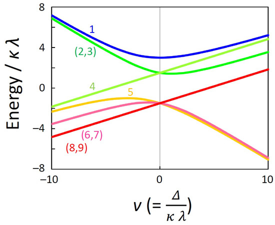
Figure 1.
Energy diagram of the nine states of the term ( = 100 cm−1, = 1).
2.2. Magnetic Susceptibility and Magnetization Equations
The temperature dependence of the magnetic susceptibility can be obtained by the Van Vleck formula [12], using the above energy equations and the Zeeman coefficients, where k represents the Boltzmann constatnt. This is a zero-field susuceptibility equation.
The field-dependent magnetic susceptibility equation can be expressed as follows, where represents the magnetic field. This equation is valid when the magnetic field is not so large.
The magnetization for the and directions, and , are expressed as follows, where represents the magnetic field.
The powder average of the magnetization is generally expressed by the following equation.
When the symmetry is axial (), the above equation can be expanded by calculating the integrals to obtain the following powder average equation.
Practically, the following equation, with Equation (82), is good enough to calculate the powder average of magnetization, if m is large enough.
2.3. Magnetic Simulation
Using the closed-form equations for zero-field energies and Zeeman coefficients, magnetic simulation is possible. Such simulation was performed for the -ground-term complexes [5,6,7], and is expected to be possible also for the -ground-term complexes if the equations derived in this study are used. Two of the examples are going to shown here. The first one is for a tetrahedral nickekel(II) complex, possessing ground term (Figure 2). Such simulation and analysis were conducted earlier [3], and the present simulation was consistent with the earlier ones. Since the nickel(II) ion has a electronic configuration, the has a negative value. In this simulation, the and were fixed to the often observed values. When the tetrahedral coordination geometry around nickel(II) ion is distorted, the v generally takes the negative values, but the simulation was also performed for the positive v values. With the variation of v, the curves systematically change. That is because the ground state is and unchanged.

Figure 2.
Theoretical T plot for tetrahedral nickel(II) complexes ( = −100 cm−1, = 0.9, v = −10, −5, 0, 5, and 10).
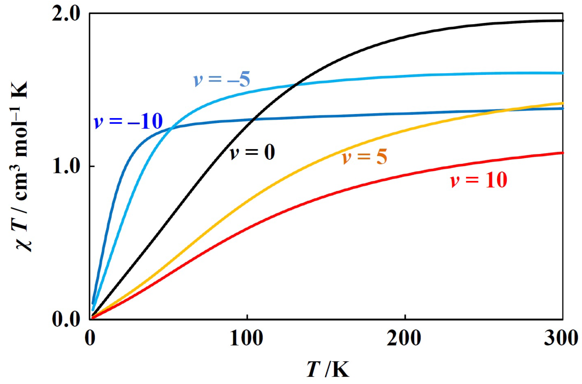
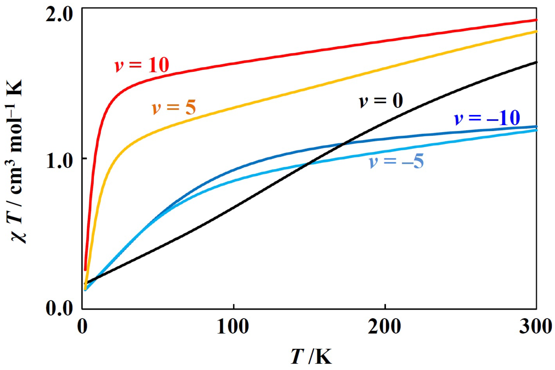
The other simulation example is for the positive case (Figure 3). This case corresponds to the octahedral vanadium(III) complexes with electronic configuraions and octahedral low-spin manganese(III) and octahedral low-spin chromium(II) complexes with electronic configurations. In these cases, takes positive values, since the metal ion has less than five d-electrons. With the variation of v, the curves drastically change. This is because the ground state changes from a doubly degenerate () state (v < 0) to a non-degenerate state (v > 0).
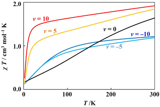
Figure 3.
Theoretical T plot for octahedral low-spin manganese(III) complexes ( = 100 cm−1, = 0.9, v = −10, −5, 0, 5, and 10).
3. Discussion
In order to obtain magnetic susceptibility and magnetization equations for the metal complexes with ground terms, the zero-field energies and Zeeman coefficients were obtained in closed form by solving the secular matrices. Fortunately, the resulting equations do not contain the imaginary part. Therefore, the equations can be easily handled, and anyone who wants to obtain Zeeman energy values and so on can calculate them without any specific programs. Using the equations, magnetic susceptibility and magnetization can be calculated simply by substituting the values of the parameters into the equations.
The metal complexes with ground terms include octahedral vanadium(III) complexes with electronic configurations, octahedral low-spin manganese(III) and chromium(II) complexes with electronic configurations, and tetrahedral nickel(II) complexes with electronic configurations. Although any new data were not analyzed in this study, the equations obtained in this study are expected to be useful in analyzing the magnetic data of the complexes, as well as the the expressions utilized in magnetic analyses [5,6,7].
The magnetic susceptibility and magnetization equations require three independent parameters, the axial splitting parameter, , the spin-orbit coupling parameter, , and the effective orbital reduction factor, . These three parameters are important in considering T-term magnetism. On the other hand, when the zero-field splitting is treated, the zero-field splitting parameter, D, is used. Since the normal zero-field splitting occurs as the result of the spin-spin interaction in the system, this interaction is different from the spin-orbit interaction. Therefore, the different parameter system was used in this study. Of course, [, , v ()] is also a good parameter set for the T-term magnetism.
4. Materials and Methods
The procedure of handling the wave functions of the term was well described by Kahn [11] to obtain zero-field energies and Zeeman coefficients. His method was basically used for the term in this study, obtaining zero-field energies and Zeeman coefficients. Therefore, the detailed method is described in reference [11]. The only difference is the definition of ”v”. That is, Kahn defined , while v was defined as in this study. Fortunately, there was no difficulty in solving the matrices in closed form. The code including the obtained equations was written on REALbasic software [13]. Calculations were conducted by MagSaki(3T1) ver.0.0.1 software developed using REALbasic software [13].
5. Conclusions
The zero-field energies and Zeeman coefficients were obtained in closed form for the distorted metal complexes with ground term. The magnetic susceptibility and magnetization equations were also obtained. Using the equations, magnetic susceptibility and magnetization can be calculated simply by substituting the values of the parameters into the equations. The equations are useful for -ground-term complexes, including octahedral vanadium(III), octahedral low-spin manganese(III), octahedral low-spin chromium(II), and tetrahedral nickel(II) complexes.
Funding
This research was funded by Japan society for the promotion of science (JSPS) KAKENHI grant number 15K05445.
Acknowledgments
Financial support by Yamagata University is acknowledged.
Conflicts of Interest
The author declares no conflict of interest.
References
- Figgis, B.N. The magnetic properties of transition metal ions in asymmetric ligand fields. Part 2.—Cubic field 3T2 terms. Trans. Faraday Soc. 1961, 57, 198–203. [Google Scholar] [CrossRef]
- Lines, M.E. Magnetic Properties of CoCl2 and NiCl2. Phys. Rev. 1963, 131, 546–555. [Google Scholar] [CrossRef]
- Figgis, B.N.; Lewis, J.; Mabbs, F.E.; Webb, G.A. The magnetic behaviour of cubic field 3T1g terms. J. Chem. Soc. A 1966, 1411–1421. [Google Scholar] [CrossRef]
- Figgis, B.N.; Lewis, J.; Mabbs, F.E.; Webb, G.A. The magnetic behaviour of cubic field 5T2g terms in lower symmetry. J. Chem. Soc. A 1967, 442–447. [Google Scholar] [CrossRef]
- Sakiyama, H.; Ito, R.; Kumagai, H.; Inoue, K.; Sakamoto, M.; Nishida, Y.; Yamasaki, M. Dinuclear Cobalt(II) Complexes of an Acyclic Phenol-Based Dinucleating Ligand with Four Methoxyethyl Chelating Arms—First Magnetic Analyses in an Axially Distorted Octahedral Field. Eur. J. Inorg. Chem. 2001, 2001, 2027–2032. [Google Scholar] [CrossRef]
- Sakiyama, H.; Adams, H.; Fenton, D.E.; Cummings, L.R.; McHugh, P.E.; Ōkawa, H. Magnetic analyses of isosceles tricobalt(II) complexes containing two types of octahedral high-spin cobalt(II) ions. Open J. Inorg. Chem. 2011, 1, 33–38. [Google Scholar] [CrossRef]
- Sakiyama, H.; Powell, A.K. Magnetic analysis of a tetranuclear octahedral high-spin cobalt(II) complex based on a newly derived magnetic susceptibility equation. Dalton Trans. 2014, 43, 14542–14545. [Google Scholar] [CrossRef] [PubMed]
- Mabbs, F.E.; Machin, D.J. Magnetism and Transition Metal Complexes; Chapman and Hall: London, UK, 1973; pp. 165–167. [Google Scholar]
- Sakiyama, H. Theoretical equations of Zeeman energy levels for distorted metal complexes with 5T2g ground terms. J. Math. Chem. 2018. [Google Scholar] [CrossRef]
- Griffith, J.S. The Theory of Transition-Metal Ions; Cambridge University Press: Cambridge, UK, 1961; pp. 340–374. [Google Scholar]
- Kahn, O. Molecular Magnetism; VCH: New York, NY, USA, 1993; pp. 38–43. [Google Scholar]
- Van Vleck, J.H. Theory of Electric and Magnetic Susceptibilities; Oxford University Press: Oxford, UK, 1932; pp. 181–202. [Google Scholar]
- REAL Software, Inc. 1996–2006. Available online: http://www.realsoftware.com/ (accessed on 25 February 2019).

© 2019 by the author. Licensee MDPI, Basel, Switzerland. This article is an open access article distributed under the terms and conditions of the Creative Commons Attribution (CC BY) license (http://creativecommons.org/licenses/by/4.0/).