Abstract
Hāpuku (Polyprion oxygeneios) is a promising candidate for aquaculture production in New Zealand. Methods for spawning, juvenile production, and growout to harvest entirely on land, where water quality, pathogens, environmental impacts, and genetic “pollution” can be tightly controlled, have been developed, and genetic improvement to optimise land-based production is the obvious next step. However, estimates of genetic parameters are required to design a rigorous, disciplined, and effective selective breeding program. By using existing data consisting of irregularly spaced repeated measurements of fork length and live body weight collected on wild-collected founders and two generations of captively reared progeny, we evaluated the species’ genetic potential for improvement in growth. We first tested a range of univariate random regression models to identify the best-fitting models for these data. Subsequently, using a bivariate model, we estimated variance components for growth trajectories of fork length and whole body weight. With one to six records available per fish, the best-fitting univariate models included only a fixed effect for contemporary groups and fixed and random genetic third-order Legendre polynomials. More complex models that included full-sib family and/or permanent environmental effects produced unacceptable constrained and/or non-positive-definite solutions. Both traits are moderately heritable at all stages of the growout phase (~0.4–0.5), and the genetic correlation patterns between daily breeding values estimated via the covariance function are different for length and weight. Genetic correlations for length between all pairs of age-specific breeding values are positive and strong (>0.7) and change gradually and smoothly with increasing temporal separation. For weight, these correlations deteriorate more rapidly with increasing time lags between measurements and become negative for some age pairings. We conclude that random regression analyses are a valuable tool for extracting genetic information from irregularly spaced repeated measurements of fish size, speculate that emerging technologies for high-throughput genotyping and phenotyping will add to the value of this approach in the near future, and reason that a breeding strategy that rigorously takes into account the potentially unfavourable genetic correlations between breeding values for weight at some ages will further adapt hāpuku to land-based systems and enhance the profitability commercial-scale production.
Keywords:
Polyprion; hāpuku; land-based aquaculture; genetic improvement; selective breeding; variance components; random regression; variance function Key Contribution:
These are the first and, to date, only genetic parameter estimates for hapuku; they demonstrate that growth in land-based systems is amenable to genetic improvement through selective breeding.
1. Introduction
Polyprion oxygeneios (Polyprionidae; Nelson, 1994 [1]), one of only two species in the genus, is generally known in New Zealand by its Māori name, hāpuku, or its common name, groper. The species is widely distributed in the southern hemisphere, occurring in southern Australia, southern Brazil, South Africa, Chile, and New Zealand at depths between 50 and 900 m [2,3,4], and has also been reported in the south-west Atlantic [5]. Hāpuku is a large, slow-growing species that can live for 60 years, reach up to 160 cm in total length, and weigh over 100 kg. Hāpuku reaches sexual maturity at around seven years of age [4,6], and growth is rapid during the first three years of life but slows considerably thereafter [7,8]. The species is highly valued by recreational and commercial fishers for its good flavour, flesh quality, and texture. However, catches in New Zealand are relatively low, with a total allowable commercial catch of ~1000–2000 metric tons annually under the New Zealand Fisheries quota management system [9,10].
There is global interest in Polyprion aquaculture [11,12,13], and hāpuku’s rapid early growth, high market value, and limited supply have attracted interest from the New Zealand aquaculture sector, which is striving to reach a government-set sales target of NZD 3 billion by 2035. Achieving this ambitious objective will require diversifying both the species farmed and the production systems used to grow them, with a focus on high-value species for domestic and export markets. While offshore sea cage farming is receiving a great deal of attention in New Zealand [14], the risks of escapees breeding with wild fish, the potential for detrimental environmental impacts from waste and damaged gear, and concerns over animal welfare, some countries are limiting or banning the practice in favour of closed pens and land-based production systems where biosecurity, pathogens, water quality, and waste products can be tightly controlled. To enable and de-risk the potential for land-based hāpuku production, New Zealand’s National Institute of Water and Atmospheric Research (NIWA) has, since 2002, pioneered reliable methods to condition and spawn captively reared broodstock, as well as land-based hatchery, juvenile, and growout methods (see [8] for a review).
To date, NIWA’s captive breeding and domestication program for hāpuku has generated over 100 G1 broodstock from wild-collected G0 parental stocks [8]. This, in conjunction with breakthroughs in spawning and larval-rearing techniques, provides a solid platform for genetically rigorous and disciplined selective breeding. From an economic perspective, growth rate and feed conversion efficiency are generally the highest priority traits for improvement in farmed fish species, at least initially [15]. Faster growth shortens the time to market and, in many fish species, leads to more efficient feed conversion [16,17,18,19,20,21], although there are notable exceptions [22].
Growth is a dynamically expressed quantitative trait [23] that varies temporally and responds to a range of environmental conditions such as temperature, water quality parameters, and feeding on a continuous time scale. Such traits are also often referred to as infinite-dimension traits that can be efficiently evaluated using mixed model random regression (RR) approaches to characterise their dynamics at the genetic level [24]. However, most fish breeding programs select for growth based on genetic variation in endpoint assessments, typically whole fish weight, filet yield and other production traits measured at harvest.
Furthermore, RR approaches can estimate the heritabilities and breeding values of growth traits at any age estimated via covariance functions and improve the accuracy of breeding values by exploiting more information [25,26]. Importantly, the random coefficients estimated using these models do not correspond directly to the genetic value for a specific phenotype, but rather the temporal pattern in predicted additive genetic value as a function of a continuous independent variable (typically age), and thus predict individual-level genetic trajectories of the trait(s) over time. In cultured fish, random regression analyses have been applied mostly to tilapia [27,28,29,30,31,32,33] but also to rainbow trout [34,35], Japanese flounder [36], and turbot [37]. These studies all conclude that this approach can be more efficient than measuring growth-related traits at specific ages. Furthermore, emerging technologies, in particular high-throughput phenomics, will soon be generating high-resolution time-series data for cultured fish amenable to random regression analysis (see [38] for a review).
The objective of this study is to explore the potential for implementing random regression models to estimate variance components and breeding values for growth traits in hāpuku raised in a land-based aquaculture system using pre-existing weight and length data collected at irregularly spaced points over an extended period during the initial phases of domestication of the species [39].
2. Materials and Methods
2.1. Experimental Population and Rearing Conditions
All fish rearing and data collection were conducted at the NIWA Northland Aquaculture Centre, Ruakākā, New Zealand (previously known as the Northland Marine Research Centre and Bream Bay Aquaculture Park when the data were collected).
We produced the experimental fish in three spawning seasons. Parents for the first two spawning seasons (2008 and 2010) were collected from the wild using hook and line from the east coast of northern New Zealand and from Cook Strait and spawned naturally in groups during their natural antipodal spring/summer spawning season (September–December). Parents for the 2013 spawning season were the captively reared progeny of the 2008 wild fish that had been raised in 20 to 70 m3 circular tanks with a nearly natural photoperiod and thermal regime (either two weeks or eight weeks advanced compared to ambient/natural). Sea water temperature ranged from a minimum of 10.0–12.5 °C prior to spawning to a maximum of 17–19 °C in summer. During spawning, broodstock was maintained at between 10 and 13.5 °C. Fertilised eggs were collected from the surface of the tanks by directing the outflow from the group spawning tank through a fine mesh screen suspended in an overflow box.
We incubated eggs and yolk-sac larvae in 400 L conical-bottomed tanks supplied with filtered, UV-disinfected, and oxygenated seawater at 14–19 °C. After the onset of exogenous feeding, we transferred larvae to circular nursery tanks (5 or 10 m3) and initially fed them enriched rotifers using a semi-static green water rearing protocol [40,41,42,43] followed by enriched Artemia. Following the transition to Artemia, water flows increased, and the addition of algae ceased. Rotifer and Artemia enrichments included Red Pepper (Bern Aqua, Olen Belgium) and Selco® S.presso (Inve, Dendermonde, Belgium).
At ~50 days post-hatch (dph), the feeding larvae were weaned onto commercial dry feed (O-range [Inve, Dendermonde, Belgium]). Weaned juveniles were then transferred to 10 m3 flow-through tanks under ambient photothermal conditions and fed continuously to satiation on O-range (Inve, Dendermonde, Belgium) and/or NovaME (Skretting, Boxmeer, The Netherlands) commercial diets. We implanted the fish with passive integrated transponder (PIT) tags at ~60 g and periodically split/transferred the groups to larger tanks (20 to 70 m3) as they grew larger to avoid over-crowding, but the spawning-event specific progeny groups were never graded or mixed. Consequently, all fish measured from the same tank on the same date had experienced the same environmental and feeding conditions for their entire lives and were treated as contemporary groups in the genetic analyses (see Section 3.5 below).
2.2. Data Collection
Individual fork length and whole-body weight (hereafter referred to simply as length and weight) were collected from each fish starting from tagging. Before we measured them, we anesthetised all fish using either 2-phenoxyethanol at 200–400 ppm or Aqui-S at 20–40 ppm. Weight measurements were to the nearest g for all fish, and length to the nearest mm for fish under 300 g, and to the nearest 0.5 mm thereafter. We measured fish several times throughout their lives, but due to wider operational requirements at the site and other contemporaneous projects, these measurements were irregularly spaced, and the number of measurements varied between groups.
2.3. Genotyping and Parentage Assignment
Genotyping and parentage assignment protocols have been published previously [39], but briefly, we extracted DNA from fin clips collected from parents and progeny and preserved in ≥70% ethanol. Fin clips were then sent to AgResearch (Mosgiel, New Zealand) for processing, genotyping, and parentage assignment.
The marker panel consisted of nine multiplexed microsatellite markers. The PCR annealing temperature was 56 °C with a MgCl2 concentration of 2.0 mM. The primer concentrations ranged from 0.1 µM to 0.6 µM (see Supplementary Table S1 for details). AgResearch analysed the amplification products using fluorescently labelled primers and an ABI3730 genetic analyser (Applied Biosystems, Foster City, CA, USA) They scored allele sizes using the GeneScan™ –500 LIZ® Size Standard and GeneMapper Software v.3.7 (both Applied Biosystems, Foster City, CA, USA).
AgResearch also reconstructed pedigrees using a proprietary pedigree analysis program (K.G. Dodds, pers. comm.) that compares the DNA profiles of the progeny against all combinations of parents within the spawning tank. The probabilities and limits of detection were calculated to assist in the parentage analysis. Over 95% of progeny could be assigned to a unique parental pair.
2.4. Data Quality Control and Editing
We used the R statistical computing software version 4.3 [44] for all data processing, statistical analyses, and plots.
The raw dataset consisted of 25,103 records on 5343 individual fish. After they were older than 600 days post-hatching (dph), many of these fish were used in experiments aimed at inducing sexual maturity and spawning that involved hormonal and photoperiod manipulation [45,46]. Furthermore, hāpuku reached the target harvest size in 12–18 months. Consequently, we dropped all records with dph > 600 from the dataset. In addition, exploratory analyses revealed that the weight and length records for many of the fish weighing less than 50 g and 150 mm in length showed no within-assessment variation and were not individual measurements, but contemporary group means. We, therefore, also removed records for these small fish. Finally, we removed all records for contemporary groups with 10 or fewer records because these records were from intermittent (and in some cases lethal) sub-sampling rather than full assessments and contemporary group means based on such small sample sizes are unreliable. After these edits, the final dataset consisted of 16,733 records on 5252 fish derived from 16 spawning events involving a total of 27 sires and 20 dams. These spawns generated 108 unique full-sib (FS) families (Table 1). We retained data from 79 of the original 129 contemporary groups/sampling events between 2009 and 2014 (Supplementary Table S2).

Table 1.
Summary of spawning/hatching events that produced the evaluated fish. The number of sires and dams represented in the group, number of full-sib (FS) families, and number of individual progeny produced. Because some sires and dams contributed to multiple spawning events, potentially even mating with the same partners, the sires, dams, and family totals are not column sums.
We used the R-package pedantics (https://github.com/cran/pedantics, accessed on 23 June 2024) to visualise the pedigree and summarise the relationships for the 5252 fish with phenotypic records and their wild (G0) parents without records. Figure 1 presents the individual-level pedigree. The vast majority of the measured fish were G1 progeny produced in the 2008 and 2010 spawns of G0 parents. Consequently, most of the information available is in the form of full and half-sib relationships within the G1 generation, although the data included some trans-generational relationships involving the G2 progeny produced in 2013. Supplementary Table S3 summarises the number of individuals in all relationship classes present in the pedigree.
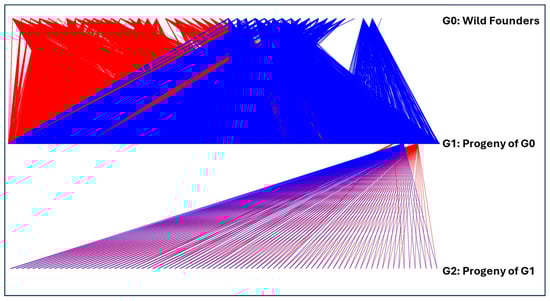
Figure 1.
Pedigree diagram of all fish used in the genetic analysis. Maternal links are red; paternal links are blue.
2.5. Model Development and Genetic Parameter Estimation
We tested a total of 48 univariate random regression models (24 for each of the two growth traits) using ASReml-R v 4.2 [47] and the asremlPlus R- package (https://CRAN.R-project.org/package=asremlPlus, accessed on 20 June 2024). All 48 models included fixed Legendre polynomials representing the population mean growth curve [35] and a categorical fixed effect of the contemporary group (assessment × tank) to account for systematic differences in group means caused by shared differences in rearing conditions. All models also included random direct additive genetic Legendre polynomials with structure from the pedigree-derived numerator relationship matrix. Beyond these effects, we systematically varied the inclusion of (1) random categorical full-sib family effects and (2) random permanent environmental effects, which we attempted to estimate as either diagonal covariance structures that assume the correlations among the polynomials are zero or as unstructured matrices to estimate these correlations. The full-sib family effect combines maternal (genetic), non-additive genetic, and common environmental effects. Permanent environmental effects account for the residual covariance between repeated measurements. Finally, we varied the order of both the fixed and random Legendre polynomials from zero to three, with the orders of all polynomials included in a single model being equal. The general form of these models is as follows:
in which is the vector of observations; is the vector of fixed effects; a is the vector of random coefficients for direct additive genetic effects; is the vector of random coefficients for full-sib families; is the vector of permanent environmental effects; ɛ is the vector of residual effects; and , , and are incidence matrices that associate individuals with specific levels of the fixed and random effects. This model is based on the following assumptions:
in which is the matrix of expectations for fixed and random effects; is the matrix of (co)variances; and are (co)variance matrices between random regression coefficients (of order equal to the order of the polynomial used) for direct additive genetic, full-sib family, and permanent environmental effects, respectively; is the additive genetic numerator relationship matrix; is an identity matrix; is the number of animals for which records are available; ⊗ is the Kronecker product between matrices; and is a matrix of residual variances. Not all models included all the random terms, and as mentioned above, we used two different structures for (diagonal and unstructured). The complete range of models evaluated is presented in Table 2 Supplementary File S1 provides example R scripts for fitting the various models.
Table 2.
Summary of the models evaluated. Columns represent the full range of possible fixed and random Legendre (Leg) polymonials. Rows represent specific models with the highest degree for each of the possible model terms. PE = permanent environmental effects; US = unstructured; DIAG = diagonal structure.
To compare the goodness of fit between models with different fixed effects (i.e., different orders of the fixed Legendre polynomials), we estimated the Aikeke information criterion (AIC) and Bayesian information criterion (BIC) for each model based on its full likelihood using the approach developed by Verbyla [48] and implemented as the infoCriteria() function in the asremlPlus package (https://CRAN.R-project.org/package=asremlPlus, accessed on 23 June 2024). Based on these criteria and on the constraints imposed on variance components by the ASReml-R solver caused by limitations in the dataset (see Section 3), we identified the preferred univariate model for each trait (lowest AIC and BIC; highest log-likelihood; no constrained or non-positive-definite components).
To more accurately estimate variance components and breeding values, we next fit a bivariate model using the same order Legendre polynomials as the preferred univariate models, again using ASReml-R v 4.2 [47]. After thus estimating the covariance matrices for the random Legendre polynomials, we estimated the genetic and phenotypic variances and heritabilities for weight and length at ranging from 50 to 400 at 10-day intervals based on the covariance function [49,50,51].
We used variations on R functions available at http://morotalab.org/UFV2019/day3/day3.html#9 (accessed on 10 June 2024) (Supplementary File S2) to transform the data to a −1 to 1 scale and calculate the normalised orthogonal Legendre polynomials according to the following expressions:
Standardised at i sampling points:
where max(dph) and min(dph) are the maximum and minimum values of in the dataset.
Legendre polynomials (Φ) of order 0–3 calculated for all values of as follows:
where is any of the (standardised) values at which the trait was measured, and is the order of the mth polynomial of order .
We estimated the additive genetic (co)variance between any pair of transformed dph values as follows:
where is the mth degree Legendre polynomial evaluated at dph = k. If the result is the genetic variance for dphi, and genetic covariances between dphi and dphj if .
Because the bivariate model we fit estimated a single residual variance component for each trait, we separately calculated the heritabilities (h2) for length and weight at each dph as follows:
We further estimated the genetic correlations between all pairs of as follows:
where i and j are indices for at all sampling points.
3. Results and Discussion
3.1. Mating Success and Parental Contributions
Figure 2 shows the numbers of progeny and the number of mates for each of the sires and dams that produced surviving progeny at tagging. The contributions of individual parents are highly heterogeneous (Figure 2a,b), with small numbers of sires and dams highly represented and the majority making lower genetic contributions to the progeny population. The number of mates per dam (Figure 2d) is more evenly distributed than mates per sire (Figure 2c), although a few dams mated with small numbers of sires. See Figure 1 for the pedigree.
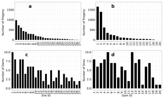
Figure 2.
Distribution of the numbers of progeny evaluated for each sire (a) and dam (b) and their numbers of mates (c,d).
While the observed level of variation in parental contributions and numbers of matings is less than ideal for a selective breeding program, it is manageable. The historical data we used for our analyses were generated using now outdated and expensive genotyping technology (nine multiplexed microsatellite markers and Sanger sequencing). Since these data were collected, higher throughput sequencing technologies have made it possible to characterise many more single nucleotide polymorphisms much more cost-effectively (see [52] for a recent review). These technologies include shotgun and targeted variations on genotyping-by-sequencing, low-coverage whole genome sequencing, and low-density SNP chips.
While developing alternative spawning strategies to balance parental contributions would be preferable, one potential approach for managing variable parental contributions in group mating species like hāpuku could be genotyping a large number of prospective selection candidates at an early stage using a low-cost genotyping approach to either reconstruct their pedigree or estimate all pairwise relationships using markers and using those data to assemble a smaller pool of selection candidates with more balanced contributions at tagging using, for example, optimal contributions approaches [53,54,55].
3.2. Phenotypic Data
A majority of the 5252 individual fish in the experimental population were measured between three and six times, but a substantial fraction was only measured once or twice (Figure 3). One of the advantages of random regression models is that they can make efficient use of repeated records data collected at irregular intervals with variable numbers of records for individuals. The historical data we analysed consisted of a limited and variable number of measurements on individuals, but we were nonetheless able to estimate genetic parameters (see below). Looking forward, however, as with genotyping, emerging high-throughput phenotyping methods, particularly those based on image analyses, are poised to revolutionise fish breeding programs. Several fish breeding programs have tested or implemented image-based phenotyping using out-of-water systems that drastically reduce the time required and costs of regular assessments, and in-water systems that collect dense time series data are under development (J. Bastiaansen, pers. comm.). Random regression approaches will undoubtedly be key to efficiently exploiting high-resolution time series data for genetic improvement.
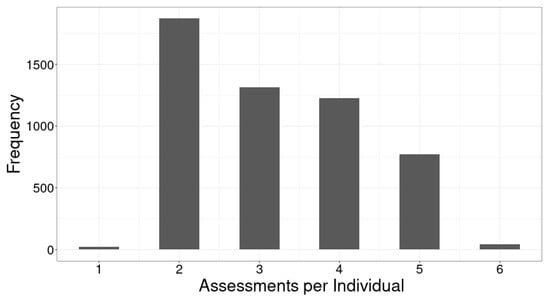
Figure 3.
Distribution of the number of assessments per individual.
Figure 4 presents the phenotypic growth trajectories for length (a) and weight (b) of the fish in the final dataset. Visually, the growth trajectory for weight is potentially slightly sigmoid/cubic, whereas the growth trajectory for length appears more quadratic. These overall patterns of growth suggest that relatively low-order polynomial regressions should be sufficient to model the genetic components of variation.

Figure 4.
Growth trajectories for body standard length (a, blue) and weight (b, black). Boxes represent contemporary groups; box widths are proportional to sample size (see Table 1 for values), and trend lines are third-order polynomials.
3.3. Genetic Model Selection
Table 3 summarises the various goodness of fit statistics for the 24 models we evaluated for each of the two traits. Model numbers and descriptions follow Table 4. “Constrained Boundary Effects” are variance components that the ASReml-R solver codes as “B” indicating that it prevented a solution falling outside the “boundary” of allowable values (e.g., negative variance components) by assigning them a small acceptable value and “Non Positive Definite Effects” are variance components the solver coded as “?”, indicating that the solution matrix is not positive-definite and, therefore, must be rejected. This is most likely due to inherent limitations of the data, specifically insufficient information to estimate some components and/or multicollinearity between them.
Table 3.
Estimated additive genetic (Vg) and residual (Vr) variances, genetic correlations (Rg), and percent of additive genetic variance explained by the component (AV%) for Legendre coefficients (standard error) from a univariate (Model #4) and bivariate model with third-order fixed and genetic Legendre polynomials for length (A) and weight (B).
Table 4.
Summary of model fitting parameters for the 24 models evaluated for length (A) and weight (B). DF = degrees of freedom for fixed effects and variance components; US = unstructured. DIAG = diagonal; PE = permanent environmental. The “Constrained Boundary Effects” column is the number of variance components that ASREML-R coded as “B”, and the “Non Positive Definite Effects” column is the number of variance components coded as “?” (see text for further explanation). The rows for the 6 best-fitting models (smallest AIC and BIC, largest log-likelihood) are in bold italic font.
The AIC and BIC presented are based on the full REML likelihood method [48], which is appropriate for comparing models with different fixed effects, such as different orders of the fixed polynomials. For both traits, the rows for the six best-fitting models (smallest AIC and BIC, largest log-likelihood) are shown in bold italic font (Models # 4, 8, 12, 16, 20, and 24). All of these models use third-order Legendre polynomials for the fixed and random regression effects (although the specifics of these effects vary between models). However, all of these models, except for Model # 4, must be rejected because at least some of the estimated (co)variances are constrained at the boundary and/or non-positive-definite. Based on this, we chose Model # 4, which uses third-order fixed and genetic Legendre polynomials as the best model for both traits and used a bivariate version of this model for the rest of our analyses.
While the RR approach was not able to fit all of the potential models without encountering data limitations that resulted in boundary constraints and/or non-positive-definite solutions (particularly models that included full-sib family and/or permanent environmental effects with polynomial orders > 0), it was able to fit simpler models with first- to third-order Legendre polynomials for fixed and direct additive genetic effects, producing estimates that aligned well with our expectations based on the overall shapes of the phenotypic growth curves (Figure 4). Excluding the potential non-additive genetic (full-sib families) and permanent environmental effects may overestimate the additive genetic (co)variances and heritabilities.
3.4. Genetic Parameter Estimates
Table 3 summarises the estimated genetic parameters for the Legendre coefficients for both traits based on both the third-order univariate and bivariate analyses. The first pattern to note is that the univariate and bivariate models produce similar genetic variance component estimates (Vg) for the polynomial coefficients for both traits, but the genetic variance estimates from the bivariate models are slightly smaller than those from the univariate models and have somewhat smaller standard errors (SE). This result is expected as the bivariate model accounts for the genetic correlations between the two traits, and the univariate models do not.
Most of the genetic variation (AV% for Vg) in the growth curves for both length and weight resides in the intercept term of the polynomials (L0), but the proportion of genetic variance explained by the linear term (L1) is larger for length than for weight (80.6 vs. 54.7%). The proportion of genetic variance accounted for by the quadratic term for length is nearly one-third that for weight (12.7 vs. 35.6%), and for both traits, the cubic terms account for even less variance (<10%). Furthermore, the intercept and linear terms show positive genetic correlations (Rg) that are moderate for length and very large for weight.
These results align well with our expectations based on the phenotypic growth curves (Figure 4), which are more linear for length than for weight. This implies that the growth curve for weight is more amenable to selection to change its shape because the higher-order polynomials that contribute to non-linearity are more genetically variable for weight than length.
Figure 5 plots the estimated genetic variances derived from the covariance functions for weight and length over the growout period analysed. For both traits, there is a consistent pattern of increasing genetic variance over time. Similarly, Figure 6 plots the estimated heritabilities for weight and length over the growout period. Both traits are moderately heritable, with the heritability for weight being slightly higher and more stable across the growout period than the heritability for length. These temporal patterns of genetic variation imply that selection on either length or weight at any age would be effective but do not address how selection at any specific age would affect other ages (see below).
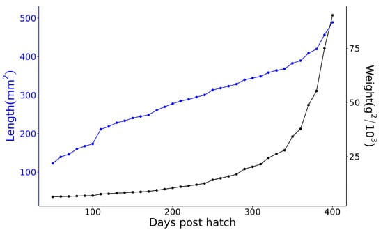
Figure 5.
Estimated genetic variance for length (blue) and weight (black) at 50–400 days post-hatch. Note that the scales for the two phenotypes differ dramatically.
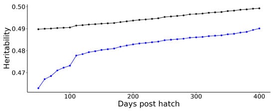
Figure 6.
Estimated heritability of length (blue) and weight (black) at 50–400 days post-hatch.
Figure 7 shows the daily breeding values for 200 randomly chosen fish. These plots illustrate two important patterns: (1) individual fish re-rank extensively over time, particularly after approximately 300 dph, and (2) the individual-level temporal patterns in breeding values show substantial variation in both their elevations and shapes, with weight showing more variation in shape than length. This is a visualisation of the differences in the AV% for the degree 0, 1, and 2 Legendre polynomials for the two traits (Table 3). Together, these two patterns suggest that selection at different ages could result in genetic improvement not only in the two growth traits at specific ages but also in the shape of the mean growth curve in the post-selection population. This has important on-farm implications, such as how to optimise feeding rates over time and how often groups of fish must be split to avoid excessive densities.
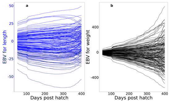
Figure 7.
Individual trajectories of EBVs for length (a) and weight (b) of 200 randomly selected individual fish.
Figure 8 presents the genetic correlations between all pairs of measurement dates from 50 to 400 days at 50-day intervals and reinforces these visual patterns quantitatively. For length (Figure 8a), the genetic correlations between all pairs of dph are positive and relatively strong (>0.7) and change gradually and smoothly with distance from the diagonal (i.e., increasing time separation between the two dph values). For weight (Figure 8b), the pattern is less regular. The correlations deteriorate more rapidly with distance from the diagonal and even become negative between some pairings of early (50, 100) and later (250–350) dph. This result differs from those of Zhao et al. [36] for turbot and of He et al. [27] for tilapia, all of whom found similar temporal patterns in time-lagged genetic correlations for weight and length and no evidence of negative correlations for either trait.
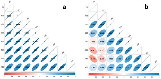
Figure 8.
Genetic correlations for length (a) and weight (b) at all pairings for dph ranging from 50 to 400 at 50-day intervals.
These temporal patterns in the genetic correlations indicate that while direct selection on length at any age will produce a reasonably large correlated response at all other ages, this is not the case for weight. Based on these estimates, the selection of weight early in the growth cycle will result in a negative response at 250–350 dph, the expected harvest time/size.
3.5. Synthesis and Prospectus
Taken as a whole, our analyses demonstrate that random regression models are a highly useful tool for estimating genetic parameters efficiently from even relatively sparse repeated records collected on multiple spawning cohorts at irregular intervals and that genetic improvement of growth in hāpuku farmed in land-based systems is likely to be highly effective. We could only fit simple models that ignored potential full-sib family (non-additive and maternal genetic) and permanent environmental variance components. Despite these limitations, our analyses support the hypothesis that the genetic variances and heritabilities (0.46–0.5) for length and weight are sufficient to support a response to selection at all stages of the growth cycle. It should be noted, however, that excluding the potential non-additive genetic and permanent environmental effects has likely led to some overestimation of the additive genetic (co)variances and heritabilities.
We also found substantial genetic variation in the shapes of temporal patterns in breeding values (i.e., the second- and third-degree polynomial coefficients; Table 3, Figure 7), particularly for weight. This indicates that it should be possible to select not only size at specific time points but also on the path by which fish achieve that size by directly selecting the breeding values of the higher-order Legendre regression coefficients.
In addition, random regression models allowed us to estimate the genetic correlations between measurements taken at different points in the growth cycle (Figure 8), a temporal analogue of the norm of reaction in genotype-by-environment interaction studies, and an important consideration for designing a disciplined and rigorous genetic improvement strategy. Interestingly, the patterns of these correlations differ markedly for the two traits. For both traits, time points separated by 50–100 days showed moderate to high genetic correlations, mostly > 0.9 for length and > 0.55 for weight. The high genetic correlations for length suggest that selecting length at any stage will produce favourable correlated responses at all stages. However, more caution will be required for selection on weight due to the more rapid decay of the genetic correlation with temporal distance and even negative genetic correlations between early and late measurements.
Finally, looking forward, although collecting repeated measurement data for cultured fish, such as the data we analysed, is currently costly, time-consuming, and stressful for the animals, this is changing rapidly. High-throughput, automated morphometric, health status, and deformity phenotyping using image analysis and other technologies are developing rapidly e.g., [56,57,58,59,60,61,62,63,64,65]). This emerging technology will undoubtedly become standard practice in the very near future, and in-cage and in-tank systems will likely produce irregularly spaced time-series data, making random regression methods an invaluable technique in fish breeders’ toolkits.
4. Conclusions
Random regression methods are seldom used but are powerful tools for estimating genetic parameters and breeding values using irregularly spaced repeated measurements of fish growth. These methods efficiently exploit all available information and make it possible to estimate key parameters for selective breeding at any age via covariance functions. In hāpuku (Polyprion oxygeneios), both length and weight are highly heritable at all phases of growout, but the genetic correlation structures between phases are different. All time-lagged genetic correlations are high and positive for length, but for weight, early and late growth is weakly or negatively correlated. Furthermore, genetic variation is second- and third-degree random regression coefficients that reveal genetic variation in the shape of growth trajectories. These methods make it possible to select the pattern of growth in addition to harvest weight in a disciplined and rigorous genetic improvement program based on repeated measurements. While acquiring such data is currently laborious and expensive, recent and near-future developments in high-throughput phenotyping, in particular automated imaging technologies, are potential game-changers that will make random regression analyses an increasingly important tool for fish breeders.
Supplementary Materials
The following supporting information can be downloaded at: https://www.mdpi.com/article/10.3390/fishes9100376/s1. Table S1: Microsatellite primers and concentrations; Table S2: Summary of contemporary groups included in the analyses; Table S3: Counts of occurrence of relationship coefficients in the A-matrix. Supplementary File S1. R code for ASReml-R analyses; Supplementary File S2. R functions for calculating standardized Legendre polynomials.
Author Contributions
Conceptualisation: J.E.S., S.P.W., A.F. and A.N.S.; Data curation, M.D.C. and G.I.; Formal analysis, M.D.C.; Funding acquisition, J.E.S., S.P.W., S.M.P. and A.F.; Investigation, M.D.C., J.E.S., S.P.W., D.M., Y.G., G.I. and A.N.S.; Methodology, M.D.C., J.E.S., S.P.W. and A.N.S.; Project administration, J.E.S., S.P.W., S.M.P., A.F. and A.N.S.; Resources, J.E.S., D.M., Y.G., G.I., S.M.P., A.F. and A.N.S.; Software, M.D.C.; Supervision, J.E.S., S.P.W., S.M.P. and A.F.; Visualisation, M.D.C.; Writing—original draft, M.D.C.; Writing—Review and editing, J.E.S. and A.N.S. All authors have read and agreed to the published version of the manuscript.
Funding
This research was funded by the New Zealand Ministry of Business Enterprise and Innovation (MBIE) Strategic Science Investment Contract C01X0705, “Increased aquaculture production through advanced broodstock development”.
Institutional Review Board Statement
The study was conducted in accordance with NIWA’s Code of Ethical Conduct and approved by NIWA’s Animal Ethics Committee (Approval no. AEC124, approval date: 11 November 2009) when animal manipulation was involved as per the NZ Animal Welfare Act 1999, and under the Farm License FW139 for activities associated with normal stock management.
Data Availability Statement
The data presented in this study are available at the request of the corresponding author, conditional on managerial approval. NIWA is a government-owned company that carries out scientific research for the benefit and economic growth of New Zealand by improving productivity and improving the sustainable use of natural resources.
Acknowledgments
We are grateful for the practical contribution of NIWA staff over the years to the long-term data collection and care of the animals. We also acknowledge and thank the various academic collaborators, in particular the University of Otago and the University of Auckland, for related projects that contributed to the dataset in this study.
Conflicts of Interest
The authors declare no conflicts of interest.
References
- Nelson, J.S. Fishes of the World, 3rd ed.; John Wiley & Sons, Inc.: New York, NY, USA, 1994; 600p. [Google Scholar]
- Paxton, J.R.; Hoese, D.F.; Allen, G.R.; Hanley, J.E. Pisces Petromyzontidae to Carangidae; Zoological Catalogue of Australia; Australian Biological Resources Survey: Canberra, Australia, 1989. [Google Scholar]
- Milessi, A.C.; Wysiecki, A.M.D.; Carvalho Filho, A.; Wiff, R. First report of the hapuku wreckfish Polyprion oxygeneios (Polyprionidae) in Argentinian waters. Lat. Am. J. Aquat. Res. 2021, 49, 354–358. [Google Scholar] [CrossRef]
- Francis, M.; Mulligan, K.; Davies, N.; Beentjes, M. Age and growth estimates for New Zealand hāpuku, Polyprion oxygeneios. Fish. Bull. 1999, 97, 227–242. [Google Scholar]
- Barreiros, J.P.; Machado, L.; Hostim-Silva, M.; Sazima, I.; Heemstra, P.C. First record of Polyprion oxygeneios (Perciformes: Polyprionidae) for the south-west Atlantic and a northernmost range extension. J. Fish Biol. 2004, 64, 1439–1441. [Google Scholar] [CrossRef][Green Version]
- Wakefield, C.B.; Newman, S.J.; Molony, B.W. Age-based demography and reproduction of hāpuku, Polyprion oxygeneios, from the south coast of Western Australia: Implications for management. ICES J. Mar. Sci. 2010, 67, 1164–1174. [Google Scholar] [CrossRef]
- Johnston, A. The southern Cook Strait groper fishery [Polyprion oxygeneios, New Zealand]. In Fisheries Technica Report; New Zealand Ministry of Agriculture and Fisheries: Wellington, New Zealand, 1983. [Google Scholar]
- Symonds, J.; Walker, S.; Pether, S.; Gublin, Y.; McQueen, D.; King, A.; Irvine, G.; Setiawan, A.; Forsythe, J.; Bruce, M. Developing yellowtail kingfish (Seriola lalandi) and hāpuku (Polyprion oxygeneios) for New Zealand aquaculture. N. Z. J. Mar. Freshw. Res. 2014, 48, 371–384. [Google Scholar] [CrossRef]
- Fisheries New Zealand. Fisheries Infosite. Available online: https://fs.fish.govt.nz/Page.aspx?pk=7&sc=HPB&ey=0 (accessed on 10 June 2024).
- Paul, L. A Description of the New Zealand Fisheries for the Two Groper Species, Hapuku (Polyprion oxygenezbs) and Bass (P. ameficanza); Ministry of Fisherie: Wellington, New Zealand, 2002.
- Papageorgiou, P. Marketing development for new Mediterranean aquaculture species: Enterprise strategies. Cah. Options Mediterr 1999, 47, 11–24. [Google Scholar]
- Mylonas, C.; Robles, R. DIVERSIFY: Enhancing the European aquaculture production by removing production bottlenecks of emerging species, producing new products and accessing new markets. Aquac. Eur. 2014, 39, 5–15. [Google Scholar]
- Quéméner, L.; Suquet, M.; Mero, D.; Gaignon, J.-L. Selection method of new candidates for finfish aquaculture: The case of the French Atlantic, the Channel and the North Sea coasts. Aquat. Living Resour. 2002, 15, 293–302. [Google Scholar] [CrossRef]
- Heasman, K.G.; Scott, N.; Ericson, J.A.; Taylor, D.I.; Buck, B.H. Extending New Zealand’s Marine Shellfish Aquaculture Into Exposed Environments—Adapting to Modern Anthropogenic Challenges. Front. Mar. Sci. 2020, 7, 565686. [Google Scholar] [CrossRef]
- Chavanne, H.; Janssen, K.; Hofherr, J.; Contini, F.; Haffray, P.; Consortium, A.; Komen, H.; Nielsen, E.E.; Bargelloni, L. A comprehensive survey on selective breeding programs and seed market in the European aquaculture fish industry. Aquac. Int. 2016, 24, 1287–1307. [Google Scholar] [CrossRef]
- Besson, M.; Allal, F.; Chatain, B.; Vergnet, A.; Clota, F.; Vandeputte, M. Combining individual phenotypes of feed intake with genomic data to improve feed efficiency in sea bass. Front. Genet. 2019, 10, 219. [Google Scholar] [CrossRef] [PubMed]
- Besson, M.; Komen, H.; Rose, G.; Vandeputte, M. The genetic correlation between feed conversion ratio and growth rate affects the design of a breeding program for more sustainable fish production. Genet. Sel. Evol. 2020, 52, 5. [Google Scholar] [CrossRef] [PubMed]
- Thodesen, J.; Grisdale-Helland, B.; Helland, S.J.; Gjerde, B. Feed intake, growth and feed utilization of offspring from wild and selected Atlantic salmon (Salmo salar). Aquaculture 1999, 180, 237–246. [Google Scholar] [CrossRef]
- Kause, A.; Tobin, D.; Houlihan, D.; Martin, S.; Mantysaari, E.; Ritola, O.; Ruohonen, K. Feed efficiency of rainbow trout can be improved through selection: Different genetic potential on alternative diets. J. Anim. Sci. 2006, 84, 807–817. [Google Scholar] [CrossRef] [PubMed]
- Ogata, H.Y.; Oku, H.; Murai, T. Growth, feed efficiency and feed intake of offspring from selected and wild Japanese flounder (Paralichthys olivaceus). Aquaculture 2002, 211, 183–193. [Google Scholar] [CrossRef]
- Dunnington, E.A.; Siegel, P.B. Long-Term Divergent Selection for Eight-Week Body Weight in White Plymouth Rock Chickens. Poult. Sci. 1996, 75, 1168–1179. [Google Scholar] [CrossRef]
- Sanchez, M.-P.; Chevassus, B.; Labbé, L.; Quillet, E.; Mambrini, M. Selection for growth of brown trout (Salmo trutta) affects feed intake but not feed efficiency. Aquat. Living Resour. 2001, 14, 41–48. [Google Scholar] [CrossRef]
- Yang, Y.; Li, R.; Li, S. An estimation method for genetic parameters of dynamic traits. Acta Vet. Et Zootech. Sin. 1996, 27, 412–416. [Google Scholar]
- Kirkpatrick, M.; Lofsvold, D.; Bulmer, M. Analysis of the inheritance, selection and evolution of growth trajectories. Genetics 1990, 124, 979–993. [Google Scholar] [CrossRef]
- Schaeffer, L.R. Application of random regression models in animal breeding. Livest. Prod. Sci. 2004, 86, 35–45. [Google Scholar] [CrossRef]
- Meyer, K. Scope for a random regression model in genetic evaluation of beef cattle for growth. Livest. Prod. Sci. 2004, 86, 69–83. [Google Scholar] [CrossRef]
- He, J.; Zhao, Y.; Zhao, J.; Gao, J.; Han, D.; Xu, P.; Yang, R. Multivariate random regression analysis for body weight and main morphological traits in genetically improved farmed tilapia (Oreochromis niloticus). Genet. Sel. Evol. 2017, 49, 80. [Google Scholar] [CrossRef]
- Rutten, M.J.M.; Komen, H.; Bovenhuis, H. Longitudinal genetic analysis of Nile tilapia (Oreochromis niloticus L.) body weight using a random regression model. Aquaculture 2005, 246, 101–113. [Google Scholar] [CrossRef]
- Turra, E.M.; de Oliveira, D.A.A.; Valente, B.D.; Teixeira, E.d.A.; Prado, S.d.A.; de Melo, D.C.; Fernandes, A.F.A.; de Alvarenga, É.R.; e Silva, M.d.A. Estimation of genetic parameters for body weights of Nile tilapia Oreochromis niloticus using random regression models. Aquaculture 2012, 354–355, 31–37. [Google Scholar] [CrossRef]
- Campideli, T.S.; Leite, N.R.; Moreira, R.L.; Abreu, L.R.A.; Campos, F.G.; Fernandes, A.F.A.; Turra, E.M.; Pedreira, M.M.; Silva, M.A.; Bonafé, C.M. Genetic sensitivity of Chitralada Nile Tilapia (Oreochromis niloticus) body weight to dietetic lysine levels. Aquaculture 2020, 528, 735530. [Google Scholar] [CrossRef]
- Fernandes, A.F.A.; Alvarenga, É.R.; Alves, G.F.O.; Manduca, L.G.; Toral, F.L.B.; Valente, B.D.; Silva, M.A.; Rosa, G.J.M.; Turra, E.M. Genotype by environment interaction across time for Nile tilapia, from juvenile to finishing stages, reared in different production systems. Aquaculture 2019, 513, 734429. [Google Scholar] [CrossRef]
- Conti, A.C.M.; Oliveira, C.A.L.d.; Martins, E.N.; Ribeiro, R.P.; Bignardi, A.B.; Porto, E.P.; Oliveira, S.N.d. Genetic parameters for weight gain and body measurements for Nile tilapias by random regression modeling. Semin. Ciências Agrárias 2014, 35, 2843–2858. [Google Scholar] [CrossRef][Green Version]
- Maldonado Turra, E.; Aparecida Andrade de Oliveira, D.; Dourado Valente, B.; de Alencar Teixeira, E.; de Assis Prado, S.; Ramos de Alvarenga, É.; Chemim de Melo, D.; Silva Felipe, V.P.; Araújo Fernandes, A.F.; de Almeida e Silva, M. Longitudinal genetic analyses of fillet traits in Nile tilapia Oreochromis niloticus. Aquaculture 2012, 356–357, 381–390. [Google Scholar] [CrossRef]
- Wang, B.; Gu, W.; Gao, H.; Hu, G.; Yang, R. Longitudinal genetic analysis for growth traits in the complete diallel cross of rainbow trout (Oncorhynchus mykiss). Aquaculture 2014, 430, 173–178. [Google Scholar] [CrossRef]
- Mckay, L.R.; Schaeffer, L.R.; Mcmillan, I. Analysis of growth curves in Rainbow Trout using random regression. In Proceedings of the Proceedings of the World Congress on Genetics Applied to Livestock Production, Montpellier, France, 19–23 August 2002. [Google Scholar]
- Zhao, J.; Zhao, Y.; Song, Z.; Liu, H.; Liu, Y.; Yang, R. Genetic analysis of the main growth traits using random regression models in Japanese flounder (Paralichthys olivaceus). Aquac. Res. 2018, 49, 1504–1511. [Google Scholar] [CrossRef]
- Yang, L.a.; Wang, L.; Wu, Z.; Hao, Z.; Song, Z.; You, F.; Yang, R. Genetic effects of ibreeding on growth trajectories in turbot (Scophthalmus maximus). Aquaculture 2021, 536, 736470. [Google Scholar] [CrossRef]
- Yu, X.; Bastiaansen, J.W.M.; Gulzari, B.; Camara, M.; Mulder, H.A.; Komen, H.; Groenen, M.A.M.; Megens, H.-J. Genome-wide association analyses reveal genotype-by-environment interactions of growth and organ weights in gilthead seabream (Sparus aurata). Aquaculture 2024, 589, 740984. [Google Scholar] [CrossRef]
- Symonds, J.; Walker, S.; Ven, I.; Marchant, A.; Irvine, G.; Pether, S.; Gublin, Y.; Bruce, M.; Anderson, R.; McEwan, K. Developing broodstock resources for farmed marine fish. Proc. N. Z. Soc. Anim. Prod. 2012, 7, 222–226. [Google Scholar]
- Palmer, P.J.; Burke, M.J.; Palmer, C.J.; Burke, J.B. Developments in controlled green-water larval culture technologies for estuarine fishes in Queensland, Australia and elsewhere. Aquaculture 2007, 272, 1–21. [Google Scholar] [CrossRef]
- Papandroulakis, N.; Divanach, P.; Anastasiadis, P.; Kentouri, M. The pseudo-green water technique for intensive rearing of sea bream (Sparus aurata) larvae. Aquac. Int. 2001, 9, 205–216. [Google Scholar] [CrossRef]
- Alves, D.; Specker, J.L.; Bengtson, D.A. Investigations into the causes of early larval mortality in cultured summer flounder (Paralichthys dentatus L.). Aquaculture 1999, 176, 155–172. [Google Scholar] [CrossRef]
- Eda, H.; Murashige, R.; Oozeki, Y.; Hagiwara, A.; Eastham, B.; Bass, P.; Tamaru, C.S.; Lee, C.-S. Factors affecting intensive larval rearing of striped mullet, Mugil cephalus. Aquaculture 1990, 91, 281–294. [Google Scholar] [CrossRef]
- R Core Team. R: A Language and Environment for Statistical Computing; R Foundation for Statistical Computing: Vienna, Austria, 2024. [Google Scholar]
- Wylie, M.J.; Setiawan, A.N.; Irvine, G.W.; Elizur, A.; Zohar, Y.; Symonds, J.E.; Lokman, P.M. Induced spawning of F1 wreckfish (Hāpuku) Polyprion oxygeneios using a synthetic sgonist of gonadotropin-releasing hormone. Fishes 2019, 4, 41. [Google Scholar] [CrossRef]
- Wylie, M.J.; Setiawan, A.N.; Irvine, G.W.; Symonds, J.E.; Elizur, A.; Dos Santos, M.; Lokman, P.M. Ovarian development of captive F1 wreckfish (hāpuku) Polyprion oxygeneios under constant and varying temperature regimes—Implications for broodstock management. Gen. Comp. Endocrinol. 2018, 257, 86–96. [Google Scholar] [CrossRef]
- Butler, D.G.; Cullis, B.R.; Gilmour, A.R.; Gogel, B.G.; Thompson, R. ASReml-R Reference Manual Version 4.2; VSN International Ltd.: Hemel Hempstead, UK, 2023. [Google Scholar]
- Verbyla, A.P. A note on model selection using information criteria for general linear models estimated using REML. Aust. N. Z. J. Stat. 2019, 61, 39–50. [Google Scholar] [CrossRef]
- Gengler, N.; Tijani, A.; Wiggans, G.R.; Misztal, I. Estimation of (co)variance function coefficients for test day yield with a expectation-maximization restricted maximum likelihood algorithm. J. Dairy Sci. 1999, 82, 1849.e1–1849.e23. [Google Scholar] [CrossRef]
- Mrode, R.A. Linear Models for the Prediction of Animal Breeding Values; CABI: Wallingford, UK, 2014. [Google Scholar]
- Meyer, K.; Hill, W.G. Estimation of genetic and phenotypic covariance functions for longitudinal or ‘repeated’records by restricted maximum likelihood. Livest. Prod. Sci. 1997, 47, 185–200. [Google Scholar] [CrossRef]
- Houston, R.D.; Bean, T.P.; Macqueen, D.J.; Gundappa, M.K.; Jin, Y.H.; Jenkins, T.L.; Selly, S.L.C.; Martin, S.A.M.; Stevens, J.R.; Santos, E.M.; et al. Harnessing genomics to fast-track genetic improvement in aquaculture. Nat. Rev. Genet. 2020, 21, 389–409. [Google Scholar] [CrossRef]
- Hinrichs, D.; Wetten, M.; Meuwissen, T.H.E. An algorithm to compute optimal genetic contributions in selection programs with large numbers of candidates. J. Anim Sci. 2006, 84, 3212–3218. [Google Scholar] [CrossRef]
- Meuwissen, T.H. Maximizing the response of selection with a predefined rate of inbreeding. J. Anim. Sci. 1997, 75, 934–940. [Google Scholar] [CrossRef]
- Meuwissen, T.H.E.; Sonesson, A.K. Maximizing the response of selection with a predefined rate of inbreeding: Overlapping generations. J. Anim. Sci. 1998, 76, 2575–2583. [Google Scholar] [CrossRef]
- Tuckey, N.P.L.; Ashton, D.T.; Li, J.; Lin, H.T.; Walker, S.P.; Symonds, J.E.; Wellenreuther, M. Automated image analysis as a tool to measure individualised growth and population structure in Chinook salmon (Oncorhynchus tshawytscha). Aquac. Fish Fish. 2022, 2, 402–413. [Google Scholar] [CrossRef]
- Vallecillos, A.; María-Dolores, E.; Villa, J.; Afonso, J.M.; Armero, E. Potential use of image analysis in breeding programs for growth and yield traits in meagre (Argyrosomus regius). J. Mar. Sci. Eng. 2023, 11, 2067. [Google Scholar] [CrossRef]
- Gulzari, B.; Mencarelli, A.; Roozeboom, C.; Komen, H.; Bastiaansen, J.W.M. Prediction of production traits by using body features of gilthead seabream (Sparus aurata) obtained from digital images. In Proceedings of the 12th World Congress on Genetics Applied to Livestock Production (WCGALP) 2412, Rotterdam, The Netherlands, 3–8 August 2022. [Google Scholar] [CrossRef]
- Gulzari, B. All Fish Deserve a Breeding Program: Designing Affordable Genomic Selection Programs with Automated Image Analysis. Ph.D. Thesis, Wageningen University, Wageningen, The Netherlands, 2023. [Google Scholar]
- Hasan, M.M.; Thomson, P.C.; Raadsma, H.W.; Khatkar, M.S. Genetic analysis of digital image derived morphometric traits of black tiger shrimp (Penaeus monodon) by incorporating G × E investigations. Front. Genet. 2022, 13, 1007123. [Google Scholar] [CrossRef]
- Liao, Y.H.; Zhou, C.W.; Liu, W.Z.; Jin, J.Y.; Li, D.Y.; Liu, F.; Fan, D.D.; Zou, Y.; Mu, Z.B.; Shen, J.; et al. 3DPhenoFish: Application for two- and three-dimensional fish morphological phenotype extraction from point cloud analysis. Zool. Res. 2021, 42, 492–501. [Google Scholar] [CrossRef]
- Gutzmann, S.B.; Hodgson, E.E.; Braun, D.; Moore, J.W.; Hovel, R.A. Predicting fish weight using photographic image analysis: A case study of broad whitefish in the lower Mackenzie River watershed. Arct. Sci. 2022, 8, 1356–1361. [Google Scholar] [CrossRef]
- Cisar, P.; Bekkozhayeva, D.; Movchan, O.; Saberioon, M.; Schraml, R. Computer vision based individual fish identification using skin dot pattern. Sci. Rep. 2021, 11, 16904. [Google Scholar] [CrossRef]
- Pauzi, S.; Hassan, M.; Yusoff, N.; Harun, N.; Bakar, A.A.; Kua, B. A review on image processing for fish disease detection. In Journal of Physics: Conference Series; IOP Publishing: Bristol, UK, 2021; p. 012042. [Google Scholar]
- Mackvandi, B.B.; Borghei, A.M.; Javadi, A.; Minaei, S.; Almassi, M. Determination of biometric parameters of fish by image analysis. J. Bio. Environ. Sci. 2015, 6, 272–276. [Google Scholar]


Disclaimer/Publisher’s Note: The statements, opinions and data contained in all publications are solely those of the individual author(s) and contributor(s) and not of MDPI and/or the editor(s). MDPI and/or the editor(s) disclaim responsibility for any injury to people or property resulting from any ideas, methods, instructions or products referred to in the content. |
© 2024 by the authors. Licensee MDPI, Basel, Switzerland. This article is an open access article distributed under the terms and conditions of the Creative Commons Attribution (CC BY) license (https://creativecommons.org/licenses/by/4.0/).