Feature Selection for Explaining Yellowfin Tuna Catch per Unit Effort Using Least Absolute Shrinkage and Selection Operator Regression

Abstract

To accurately identify the key features influencing the fisheries distribution of Pacific yellowfin tuna, this study analyzed data from 43 longline fishing vessels operated from 2008 to 2019. These vessels operated in the Pacific Ocean region (0° to 30° S; 110° E to 170° W), with a specific focus on 25 features of yellowfin tuna derived from marine environment data. For this purpose, this study opted for the Lasso regression analysis method to select features to predict Pacific yellowfin tuna fishing grounds, exploring the relationship between the catch per unit effort (CPUE) of yellowfin tuna and multiple features. This study reveals that latitude and water temperature at various depths, particularly the sea surface temperature of the preceding and subsequent months and the temperature at depths between 300 and 450 m, are the most significant features influencing CPUE. Additionally, chlorophyll concentration and large-scale climate indices (ONI and NPGIO) also have a notable impact on the distribution of CPUE for yellowfin tuna. Lasso regression effectively identifies features that are significantly correlated with the CPUE of yellowfin tuna, thereby demonstrating superior fit and predictive accuracy in comparison with other models. It provides a suitable methodological approach for selecting fishing ground features of yellowfin tuna in the Pacific Ocean.

1. Introduction

Fishery resources are one of the vital sources of food and economic support globally. Yellowfin tuna (Thunnus albacares), belonging to the Perciformes order and Thunnus genus, are widely distributed in tropical and subtropical waters, particularly abundant in the central and western Pacific region [1]. They represent a crucial component of fisheries resources. However, in recent years, due to continuous exploitation of global fishery resources and human population growth, issues such as overfishing and inadequate fisheries management have led to a decrease in the stability of spatial and temporal distribution of fishing grounds [2], posing significant challenges to fisheries sustainability.

Yellowfin tuna are highly migratory, and their core fishing grounds are dispersed and widely distributed. Their diverse distribution in fisheries necessitates a thorough investigation into the complex relationship between yellowfin tuna activities and environmental features. It is essential to select and analyze the environmental features that affect their activities to ensure the rational exploitation and protection of yellowfin tuna resources, thereby maintaining the health of the ecosystem. This research aims to study the intricate relationship between the distribution of yellowfin tuna fisheries and environmental features by selecting and analyzing the environmental features influencing their survival [3].

Catch per unit effort (CPUE) of yellowfin tuna is a key indicator for assessing the efficiency of fishing activities and the status of resources. It represents the number of yellowfin tuna caught per unit of effort or resource input, allowing for the monitoring of dynamic changes in yellowfin tuna fishery catch rates [4]. Changes in CPUE can reflect the abundance and quality of yellowfin tuna resources, as well as the success of fishing activities. However, CPUE analysis for yellowfin tuna typically involves multiple potential influencing features, including marine environmental features, longitude, latitude, and numerous different features [5]. Therefore, a thorough analysis of the relationship between CPUE and these features is crucial for fisheries. Considering all features may lead to increased model complexity and difficulty in interpretation. Feature selection can help reduce model complexity by eliminating irrelevant features, thereby reducing the impact of noise and improving the accuracy of the model. By retaining only the most important features, the model becomes more interpretable [6].

Machine learning is an automatic learning method that automatically analyzes data and extracts patterns to perform feature selection, and it has been successfully applied in numerous fields. In this study, feature selection was conducted using Lasso (least absolute shrinkage and selection operator), which is a key technique in machine learning. In 1996, Tibshirani proposed the Lasso method, which introduces an L1 norm penalty term on the basis of ordinary least squares [7]. In the field of machine learning, Lasso is mainly used for feature selection [8], identifying features that have a significant impact on the target feature to simplify the model and improve generalization ability. This regularization method helps prevent overfitting, thereby improving model performance. It is a variant of linear regression, where some regression coefficients can be compressed to zero, thereby eliminating some features from the model [9], filtering out noise features that do not significantly contribute to the target feature, and retaining features closely related to the target feature.

In current research, Lasso has been applied in various fields. In bioinformatics and genomics, it is used to analyze large-scale gene expression data to identify genes related to specific biological states or diseases [10]. In medical research, it is used for disease risk assessment, identification of biomarkers, and patient stratification to provide personalized treatment recommendations [11]. In finance, it is used for asset pricing, risk management, credit scoring models, and macroeconomic forecasting to screen key features affecting economic indicators [12]. In signal processing, it is used for signal denoising, image processing, and compressive sensing to recover signals or images through sparse representation [13]. In climate modeling and environmental monitoring, it helps to identify features that have a significant impact on environmental changes [14]. In psychology and social sciences, it is used to study individual behavior, decision-making processes, and key influencing features in social networks [15]. In marketing and consumer research, it helps identify key features influencing consumer purchasing decisions [16]. The application scope of Lasso regression technology is extensive, not limited to the aforementioned fields, and it spans multiple research directions.

In this context, the aim of this study is to explore the relationship between the CPUE of yellowfin tuna and multiple features using the Lasso regression analysis method. This work provides new methods and perspectives for research in the fisheries sector and expands our understanding of fishery ecosystems. It also provides a case study for the application of machine learning technology in the study of fishery resources, aimed at better understanding and protecting our precious marine resources.

2. Data and Methods

2.1. Data Processing

2.1.1. Data Sources

In this study, the operational range of the longline fishing vessels targeting yellowfin tuna in the central and western Pacific Ocean (110° E to 170° W, 0° to 30° S) was chosen as the research area. Additionally, the dataset comprises approximately 18,029 data points of CPUE-related data collected over the time period from 2008 to 2019. The fishery production data used were sourced from the fishing logs of 43 ocean-going longline fishing vessels operated, including vessel names, operational dates (year/month), operational locations (longitude, latitude), and catch information (species, yield, number of tails, and number of hooks deployed, etc.). Chlorophyll-a concentration data were accurately obtained from the official National Aeronautics and Space Administration (NASA) database repository (https://oceancolor.gsfc.nasa.gov/ (accessed on 23 April 2024)). Sea level anomaly (SLA) data were sourced from the AVISO (Archiving, Validation, and Interpretation of Satellite Oceanographic data) database (https://www.aviso.altimetry.fr/en/home.html (accessed on 23 April 2024)). Eddy kinetic energy data and vertical temperature and salinity data for the 0–500 m layer were obtained from the Copernicus Marine Environment Monitoring Service website (http://marine.copernicus.eu (accessed on 23 April 2024)). The temporal resolution of environmental data was monthly, while the spatial resolution of SLA, EKE, and vertical temperature and salinity data for the 0–500 m layer was 0.25° × 0.25°, and the spatial resolution of Chlorophyll-a concentration data was 4 km. Python was used to standardize the spatial resolution of environmental data to 0.5° × 0.5° grid and match it with the catch data [17].

The large-scale climate data are all monthly data. The Southern Oscillation Index (SOI) and Arctic Oscillation Index (AOI) are sourced from the Climate Prediction Center of the National Oceanic and Atmospheric Administration (NOAA). The Pacific Decadal Oscillation Index (PDOI) is reliably sourced directly from the University of Washington’s research department (http://research.jisao.washington.edu/pdo (accessed on 23 April 2024)), and the North Pacific Gyre Oscillation Index (NPGOI) is sourced from https://data.marine.copernicus.eu/product/OMI_EXTREME_CLIMVAR_PACIFIC_npgo_sla_eof_mode_projection/description (accessed on 5 January 2024).

2.1.2. CPUE Calculation

The CPUE used to measure the efficiency of fishing activities typically represents the quantity captured per unit of time or effort. It indicates the quantity of fish caught or the amount of fishery resources harvested per unit of fishing effort (such as the number of vessels or the length of fishing nets), and it is an important indicator for evaluating the efficiency of fishing activities and the abundance of resources. CPUE is usually expressed in terms of quantity or quality and is calculated by comparing the quantity of catch with the input effort or the number of resources used. It is a widely used metric in fisheries and ecology for assessing the efficiency of fishing activities and the health status of fishery resources. A decrease in CPUE may indicate overexploitation of resources or other issues, necessitating measures to protect the resources.

CPUE is also used to study the abundance and distribution of different populations within ecosystems. By comparing CPUE data from different times and locations (longitude, latitude), ecological features and life history of species can be understood. This study divides fishing areas into 0.5° × 0.5° grids and calculates the CPUE of yellowfin tuna in each grid monthly by summarizing the operational positions, number of tails, and number of hooks deployed [18]. The calculation formula is as follows:

$${\mathrm{CPUE}}_{\left(\mathrm{i},\mathrm{j}\right)}=\frac{{\mathrm{F}}_{\mathrm{fish}\left(\mathrm{i},\mathrm{j}\right)}\times 1000}{{\mathrm{H}}_{\mathrm{hook}\left(\mathrm{i},\mathrm{j}\right)}},$$

(1)

where ${\mathrm{CPUE}}_{\left(\mathrm{i},\mathrm{j}\right)}$, ${\mathrm{F}}_{\mathrm{fish}\left(\mathrm{i},\mathrm{j}\right)}$, and ${\mathrm{H}}_{\mathrm{hook}\left(\mathrm{i},\mathrm{j}\right)}$ represent the monthly average CPUE (tails/thousand hooks), total monthly catch of fish, and total monthly number of hooks deployed in the grid of the i-th longitude and the j-th latitude fishing area, respectively.

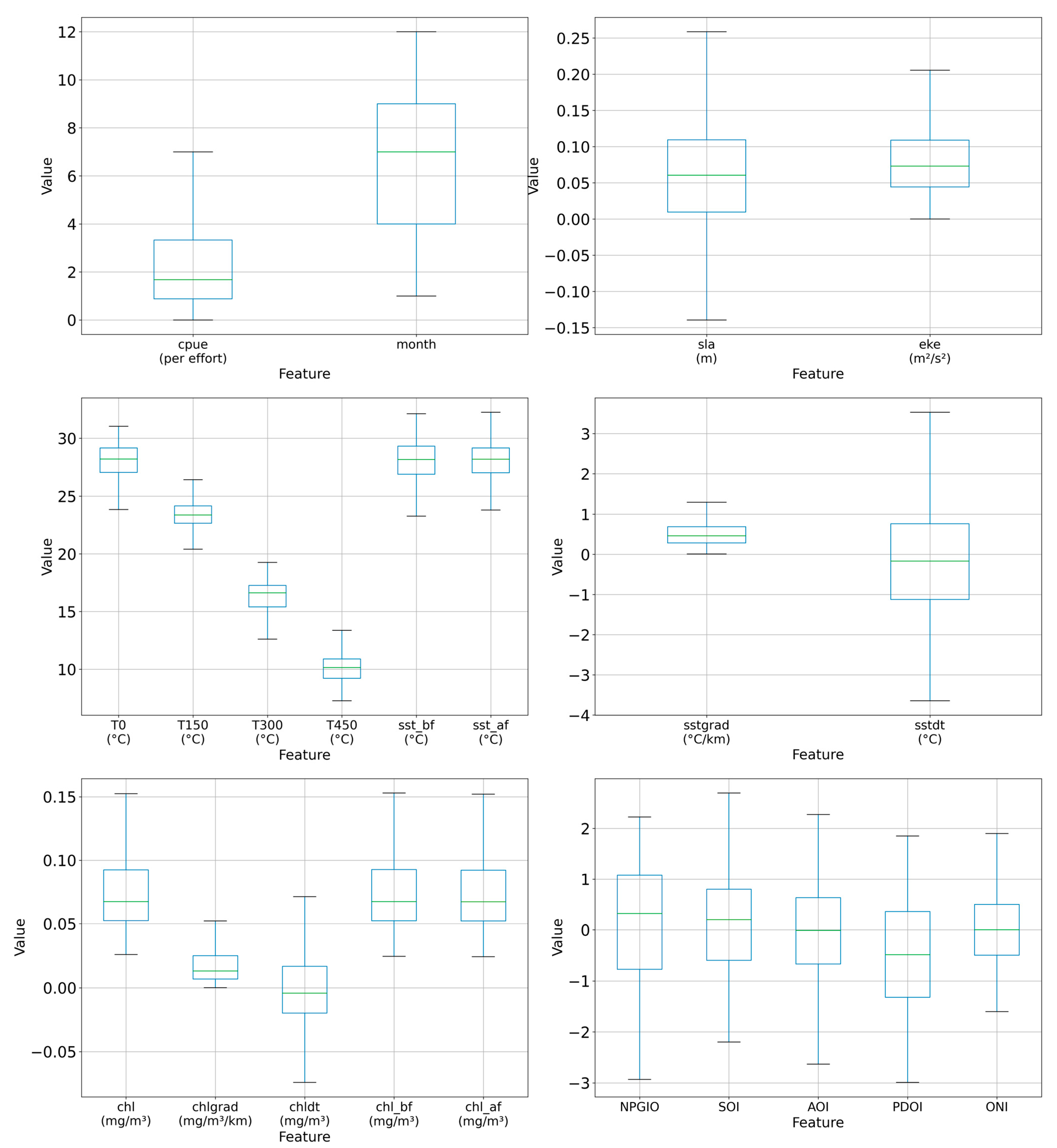
2.1.3. Data Preprocessing

The research on CPUE feature selection based on Lasso requires data collection and preprocessing to ensure the quality and availability of the data. Firstly, it is essential to identify the data sources, compute the CPUE of yellowfin tuna, and determine the relevant influencing features obtained from different channels. Subsequently, integrating data from various sources into a unified dataset is necessary for further analysis, ensuring that the dataset includes feature data corresponding to CPUE observations.

Finally, a total of 25 relevant features related to yellowfin tuna were collected and organized. The feature dataset includes the following content: CPUE, year, month, latitude (lat), longitude (lon), chlorophyll-a concentration (chl), chlorophyll concentration of the previous month (chl_bf), chlorophyll concentration of the following month (chl_af), sea surface temperature of the previous month (sst_bf), sea surface temperature of the following month (sst_af), chlorophyll anomaly (chldt), sea surface temperature anomaly (sstdt), sea temperature gradient (sstgrad), chlorophyll concentration gradient (chlgrad), sea level anomaly (sla), eddy kinetic energy (eke), sea surface temperature parameter (T0), sea temperature at 150 m depth (T150), sea temperature at 300 m depth (T300), sea temperature at 450 m depth (T450), Pacific Decadal Oscillation Index (PDOI), Southern Oscillation Index (SOI), Arctic Oscillation Index (AOI), North Pacific Gyre Oscillation Index (NPGIO), and the El Niño–Southern Oscillation Index (ONI). The numerical analysis of each feature is categorized according to temperature, chlorophyll, and ocean phenomena, as shown in Figure 1.

To analyze the distribution of various features, box plots were utilized to illustrate the statistical characteristics of the data. A box plot is an effective graphical method that describes the distribution, central tendency, and outliers of a data set. In the box plots (see Figure 1), the green line represents the median value, indicating the central tendency of the data. The blue box shows the interquartile range (IQR), which is the range between the first quartile (Q1) and the third quartile (Q3), capturing the middle 50% of the data. The whiskers extending from the box indicate the minimum and maximum values within 1.5 times the IQR from Q1 and Q3, respectively, encompassing most of the data distribution. Any data points outside this range are considered outliers and are displayed as individual points. Additionally, a black line is used to represent the actual minimum and maximum values of the data set.

2.2. Research Method

In this study, data related to yellowfin tuna CPUE were collected, including observed values of yellowfin tuna CPUE and potential features that may influence yellowfin tuna CPUE. The data were then divided into a training set (80%) and a test set (20%). A Lasso regression model was used to analyze the data, wherein irrelevant feature coefficients were shrunk to zero, thereby achieving feature selection. Python programming, version 3.10.2, was utilized for data analysis, employing relevant packages such as seaborn, scikit-learn (sklearn), math, matplotlib, and numpy to conduct feature selection and analysis. Additionally, the R language, version 4.3.0, specifically with the glmnet package, was employed for cross-validation and other methods to select appropriate regularization parameters, and the performance of the model was evaluated using the test set. Subsequently, feature selection was conducted, and the coefficients of the Lasso regression model were analyzed to determine which features had non-zero coefficients. This helped identify the degree of influence of different features on CPUE, thereby explaining the relationship between the selected features and CPUE to understand the mechanism of feature impact on CPUE. Finally, the research findings were summarized. The methodology flowchart is illustrated in Figure 2.

2.2.1. Lasso Regression Introduction

Lasso regression is a regularization technique for linear regression. As a powerful statistical analysis tool, it not only helps reduce the complexity of models to improve interpretability and predictive performance but also identifies key features in high-dimensional data for feature selection and model regularization, thus preventing overfitting. The main feature of Lasso regression is to adjust the regularization parameter to precisely shrink some coefficients to zero, achieving feature selection and effectively reducing model complexity while addressing issues like multicollinearity [19]. The computational formula for Lasso regression is as follows:

$$\mathrm{Minimize}\left(\frac{1}{2\mathrm{n}}{\sum }_{\mathrm{i}=1}^{\mathrm{n}}{\left({\mathrm{y}}_{\mathrm{i}}-{\sum }_{\mathrm{j}=1}^{\mathrm{p}}{\mathrm{x}}_{\mathrm{ij}}{\mathsf{\beta }}_{\mathrm{j}}\right)}^2+\mathsf{\lambda }{\sum }_{\mathrm{j}=1}^{\mathrm{p}}\left|{\mathsf{\beta }}_{\mathrm{j}}\right|\right),$$

(2)

In the equation, $\mathrm{n}$ is the number of samples; ${\mathrm{y}}_{\mathrm{i}}$ is the observed response variable of the i-th sample; ${\mathsf{\beta }}_{\mathrm{j}}$ is the coefficient of the j-th feature, with the intercept ${\mathrm{x}}_{\mathrm{ij}}$ being the value of the j-th feature in the i-th observation; p is the number of features (variables); λ is the regularization parameter used to control the strength of regularization. A larger λ will lead to more feature coefficients being shrunk to zero, thereby achieving feature selection.

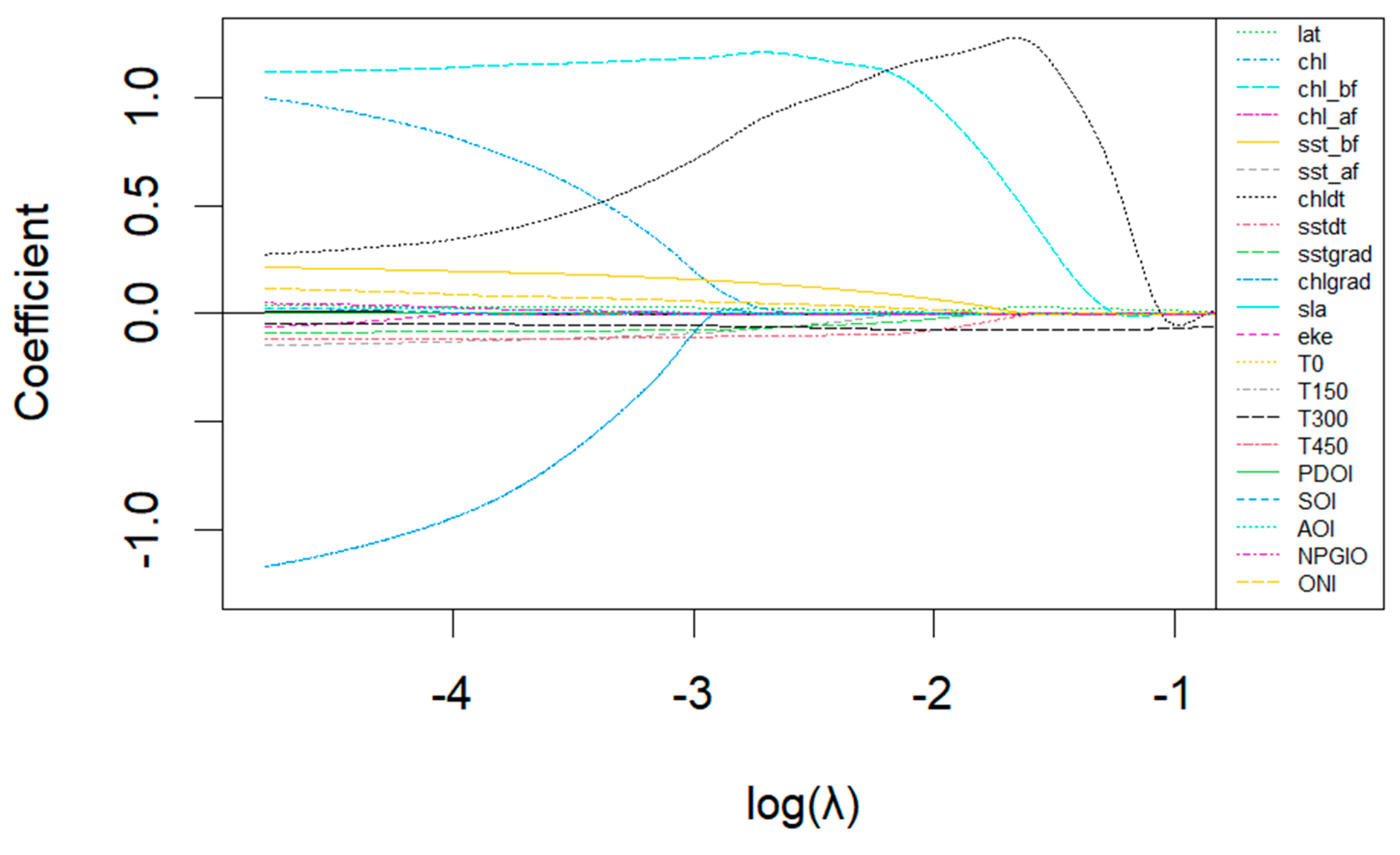
2.2.2. Screening Variables and Feature Selection

The process of Lasso variable screening and feature selection can reduce model complexity, prevent overfitting, and improve model interpretability. The steps are as follows: Load the input variables and the dependent variable needed to solve the problem, and divide the data into training and testing sets. Fit the training data to a Lasso regression model with an L1 penalty. Estimate model parameters based on the absolute values of the coefficients and their corresponding variables, selecting meaningful variables. Validate the model using the training set (80%) and the testing set (20%), assessing the accuracy of the model. For each model, calculate the average test error using cross-validation. Select the appropriate regularization parameter for Lasso regression by choosing the parameter value corresponding to the model with the smallest test error. Finally, analyze the features that may affect CPUE complex relationships using the best parameter to better understand the relationship between CPUE and various features and identify key features related to CPUE.

2.2.3. Pearson Coefficient Correlation Analysis

The Pearson correlation coefficient is a statistical method used to measure the degree of linear correlation between two variables, with values ranging from −1 to 1. A coefficient of 1 indicates a perfect positive correlation, −1 indicates a perfect negative correlation, and 0 indicates no linear correlation. In statistics, the Pearson correlation coefficient is commonly used to explore the relationship between two continuous variables. It is one of the most commonly used correlation coefficients and finds extensive application in scientific research, data analysis, social sciences, engineering, and other fields [20]. The formula to calculate the Pearson correlation coefficient ${\mathsf{\rho }}_{\mathrm{XY}}$ is as follows:

$${\mathsf{\rho }}_{\mathrm{XY}}=\frac{{\sum }_{\mathrm{i}=1}^{\mathrm{N}}{\mathrm{x}}_{\mathrm{i}}{\mathrm{y}}_{\mathrm{i}}-\frac{1}{\mathrm{N}}\left({\sum }_{\mathrm{i}=1}^{\mathrm{N}}{\mathrm{x}}_{\mathrm{i}}\right)\left({\sum }_{\mathrm{i}=1}^{\mathrm{N}}{\mathrm{y}}_{\mathrm{i}}\right)}{\sqrt{{\sum }_{\mathrm{i}=1}^{\mathrm{N}}{\mathrm{x}}_{\mathrm{i}}^2-\frac{1}{\mathrm{N}}{\left({\sum }_{\mathrm{i}=1}^{\mathrm{N}}{\mathrm{x}}_{\mathrm{i}}\right)}^2\sqrt{{\sum }_{\mathrm{i}=1}^{\mathrm{N}}{\mathrm{y}}_{\mathrm{i}}^2-\frac{1}{\mathrm{N}}{\left({\sum }_{\mathrm{i}=1}^{\mathrm{N}}{\mathrm{y}}_{\mathrm{i}}\right)}^2}}},$$

(3)

where $\mathrm{X}=\left({\mathrm{x}}_1,{\mathrm{x}}_2,\dots ,{\mathrm{x}}_{\mathrm{N}}\right),\mathrm{Y}=\left({\mathrm{y}}_1,{\mathrm{y}}_2,\dots ,{\mathrm{y}}_{\mathrm{N}}\right)$, N is the number of data points, ${\mathrm{X}}_{\mathrm{i}}$ is the i-th observation of variable X, and ${\mathrm{Y}}_{\mathrm{i}}$ is the i-th observation of variable Y.

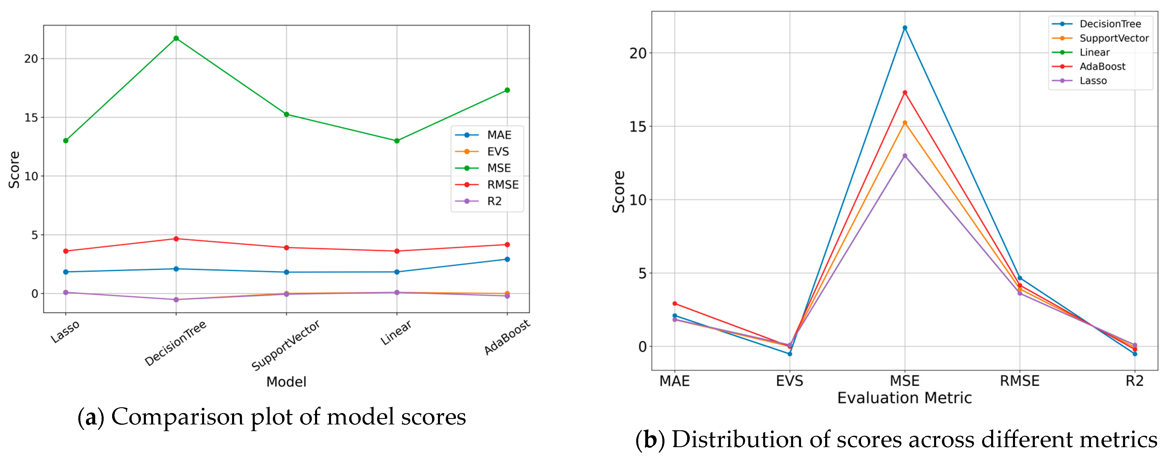
2.2.4. Model Evaluation Methods

In model prediction, several metrics can be used to measure the performance of the model. The mean absolute error (MAE) measures the average deviation of the predicted values from the actual values. The mean squared error (MSE) and the root-mean-square error (RMSE) consider the squared errors, giving larger penalties to larger errors [21]. The explained variance score measures the model’s ability to explain the variance in the data, while R-squared (coefficient of determination) is an indicator of model fit, reflecting the proportion of the variance in the data that is explained by the model. These are all metrics used in regression analysis to assess the accuracy of model predictions. These metrics are interrelated and collectively used to reflect the accuracy and generalization capability of the model. This study employs the Python packages math and scikit-learn for calculating these values. Specifically, the math package is utilized for mathematical operations, while the scikit-learn package provides tools for training and evaluating machine learning models. These values are calculated as follows:

1.

The mean absolute error (MAE) calculates the residual for each data point, taking the absolute value of each residual to ensure that negative and positive residuals do not cancel each other out. MAE is used to assess the degree of proximity between the predicted results and the actual dataset, where a smaller value indicates a better fit. The formula for MAE is as follows, where n represents the number of samples, ${\mathrm{f}}_{\mathrm{i}}$ represents the predicted value, ${\mathrm{y}}_{\mathrm{i}}$ represents the actual value, and the sum is the sum of the absolute differences between the predicted and actual values:

$$\mathrm{MAE}=\frac{1}{\mathrm{n}}\sum _{\mathrm{i}=1}^{\mathrm{n}}\left|{\mathrm{f}}_{\mathrm{i}}-{\mathrm{y}}_{\mathrm{i}}\right|$$

(4)

2.

The explained variance score (EVS) is a metric used to measure the performance of a regression model. Its value ranges from 0 to 1, where a value closer to 1 indicates that the independent variables explain the variance in the dependent variable well, while a smaller value suggests poorer performance. The formula for EVS is as follows, where y represents the true values, f represents the corresponding predicted values, and Var is the variance of the actual values:

$$\mathrm{EVS}=1-\frac{\mathrm{Var}\left(\mathrm{y}-\mathrm{f}\right)}{\mathrm{Var}\left(\mathrm{y}\right)}$$

(5)

3.

The mean squared error (MSE) is a measure of the disparity between the estimator and the estimated value. A smaller MSE indicates less difference between the predicted and actual values, reflecting better model fit. The formula for MSE is as follows, where $\mathrm{n}$ represents the total number of samples, ${\mathrm{f}}_{\mathrm{i}}$ represents the predicted value for the i-th sample, and ${\mathrm{y}}_{\mathrm{i}}$ is the corresponding true value; the sum is the squared sum of the differences between the predicted values ${\mathrm{f}}_{\mathrm{i}}$ and the true values ${\mathrm{y}}_{\mathrm{i}}$:

$$\mathrm{MSE}=\frac{1}{\mathrm{n}}\sum _{\mathrm{i}=1}^{\mathrm{n}}{\left({\mathrm{f}}_{\mathrm{i}}-{\mathrm{y}}_{\mathrm{i}}\right)}^2$$

(6)

4.

The root-mean-square error (RMSE), also known as standard error, is used to measure the deviation between observed values and true values. If there is a significant difference between predicted values and true values, the RMSE value will be large. Therefore, the standard error can effectively reflect the precision of measurements. RMSE is the square root of the sum of MSE; the calculation formula is as follows:

$$\mathrm{RMSE}=\sqrt{\frac{1}{\mathrm{n}}\sum _{\mathrm{i}=1}^{\mathrm{n}}{\left({\mathrm{f}}_{\mathrm{i}}-{\mathrm{y}}_{\mathrm{i}}\right)}^2}$$

(7)

5.

$R^2$: the coefficient of determination (R-squared) assesses the goodness of fit of the predictive model to the real data. Its value ranges from 0 to 1, where a higher value indicates less error and a better ability of the model to explain the variability of the dependent variable, implying a better fit of the model. The formula for calculating R-squared is as follows: where n represents the total number of samples, ${\mathrm{f}}_{\mathrm{i}}$ represents the predicted value for the i-th sample, ${\mathrm{y}}_{\mathrm{i}}$ represents the i-th actual observed value, and $\stackrel{\mathrm{-}}{\mathrm{y}}$ is the mean of the actual observed values. R-squared is the ratio of the sum of squared differences between predicted values and the mean of observed values to the total sum of squares.

$${\mathrm{R}}^2=1-\frac{{\sum }_{\mathrm{i}=1}^{\mathrm{n}}{\left({\mathrm{y}}_{\mathrm{i}}-{\mathrm{f}}_{\mathrm{i}}\right)}^2}{{\sum }_{\mathrm{i}=1}^{\mathrm{n}}{\left({\mathrm{y}}_{\mathrm{i}}-\stackrel{\mathrm{-}}{\mathrm{y}}\right)}^2}$$

(8)

2.2.5. Regression Model Methods

This study compares five regression models, employing the Python scikit-learn package for methodology. The scikit-learn library provides a unified interface for training various machine learning models, including decision tree regression, support vector regression (SVR), linear regression, and AdaBoost regression. Specifically, for Lasso regression modeling, we utilized the Lasso class from the scikit-learn library. DecisionTreeRegressor, SVR, LinearRegression, and AdaBoostRegressor classes are utilized for training decision tree regression, support vector regression, linear regression, and AdaBoost regression models, respectively.

Decision trees are a popular machine learning algorithm used for regression tasks. They work by recursively partitioning the data into subsets based on features that best separate the target variable. Decision tree regressors predict the target variable by averaging the target values of the training instances within each leaf node.

Support vector machine regression, SVM regression, is a powerful supervised learning algorithm used for regression tasks. It works by finding the hyperplane that best separates the data into different classes while maximizing the margin. In regression, SVM aims to find the hyperplane that best fits the data points within a specified margin of error.

Linear regression is one of the simplest and most commonly used regression techniques. It models the relationship between a dependent variable and one or more independent variables by fitting a linear equation to the observed data. The goal is to find the best-fitting line that minimizes the sum of the squared differences between the observed and predicted values.

Adaptive boosting regressor is an ensemble learning technique that combines multiple weak learners to create a strong learner. In regression tasks, AdaBoost combines multiple regression models, typically decision trees, to improve predictive performance. It iteratively adjusts the weights of incorrectly predicted instances to focus on the difficult-to-predict cases, ultimately improving the overall model’s performance.

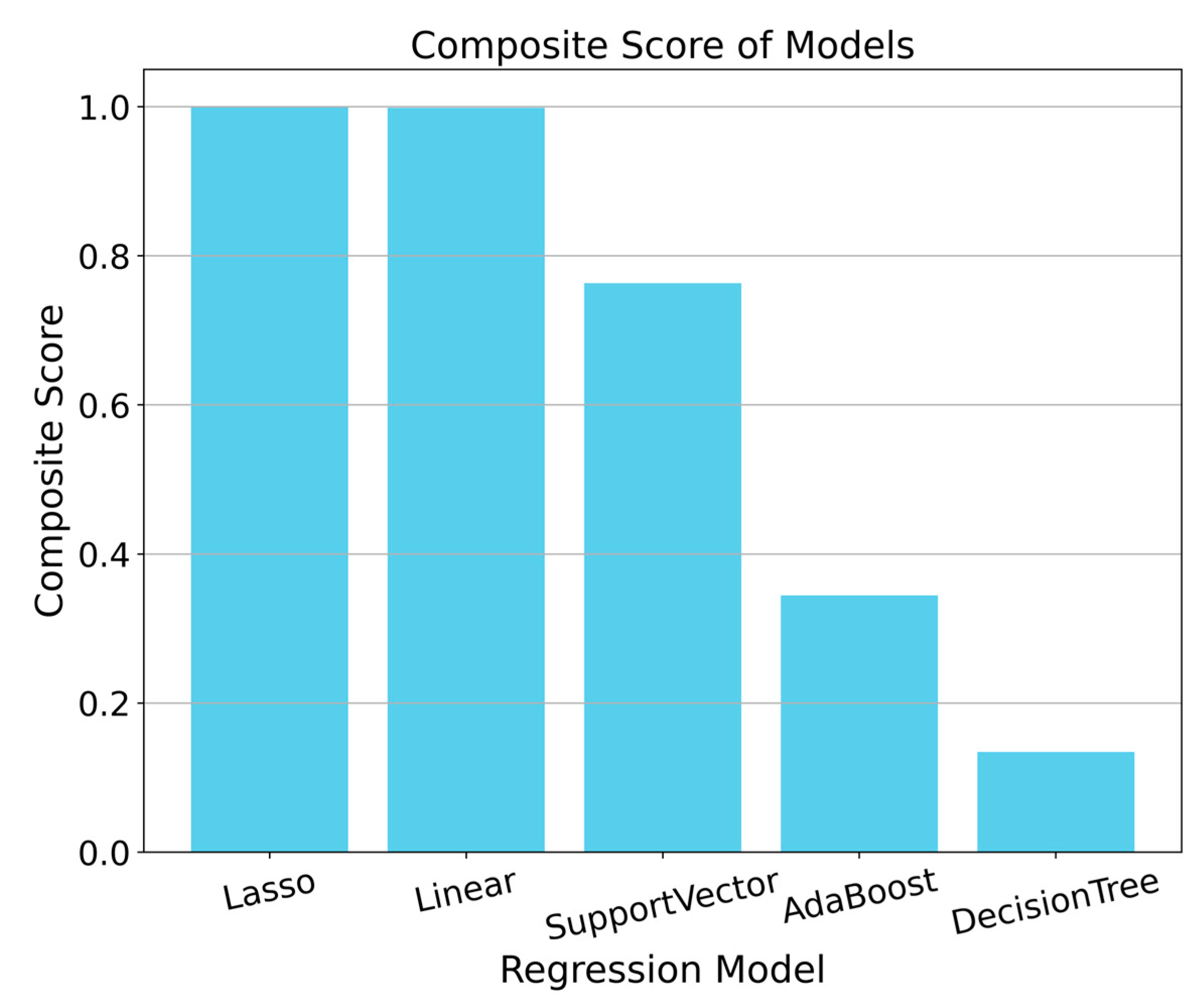
2.2.6. Comprehensive Score

To evaluate and compare the performance of these five models, a composite score was calculated based on five metrics: MAE, EVS, MSE, RMSE, and R². This composite score was derived through normalization and weighted summation of these metrics, providing a comprehensive performance evaluation index. The calculation of the composite score begins with the normalization of each metric, which involves transforming each metric’s value into a range between 0 and 1. This process aims to unify the value ranges of different metrics. Particularly for MAE, MSE, and RMSE, where smaller values indicate better performance, an inverse normalization is applied to ensure that models with lower scores receive higher ratings, reflecting superior performance. For EVS and R², where higher values denote better performance, straightforward normalization is used. The composite score is then calculated through a weighted summation, where the weights of each metric are adjusted according to their relative importance in performance evaluation, typically summing to 1. Here, the weights for MAE, MSE, and RMSE are set at 0.5/3 each, while for EVS and R², the weight is set at 0.25. This weighting reflects a holistic consideration of the models’ multifaceted performance. The composite score can be expressed by the formula, where ${\mathrm{x}}_{\mathrm{i}}$ represents the score of the i-th model on a given metric, and ${\mathrm{X}}_{\mathrm{i}}$ represents the set of scores for all models on that metric.

$$\mathrm{Score}=\left(\sum _{\mathrm{i}\in \left\{\mathrm{MAE}, \mathrm{MSE}, \mathrm{RMSE}\right\}}\left(1-\frac{{\mathrm{x}}_{\mathrm{i}}-\min \left({\mathrm{X}}_{\mathrm{i}}\right)}{\max \left({\mathrm{X}}_{\mathrm{i}}\right)-\min \left({\mathrm{X}}_{\mathrm{i}}\right)}\right)\times \frac{0.5}{3}\right)+\left(\sum _{\mathrm{i}\in \left\{\mathrm{EVS}, {\mathrm{R}}^2\right\}}\frac{{\mathrm{x}}_{\mathrm{i}}-\min \left({\mathrm{X}}_{\mathrm{i}}\right)}{\max \left({\mathrm{X}}_{\mathrm{i}}\right)-\min \left({\mathrm{X}}_{\mathrm{i}}\right)}\times 0.25\right)$$

(9)

3. CPUE Feature Selection Analysis Results

3.1. Correlation Analysis between CPUE and Features

The Pearson correlation coefficient is commonly used to display the correlation between a series of features, making it highly useful for data analysis and feature selection. The calculations were conducted using the seaborn package in Python. This coefficient measures the strength of the linear relationship between two features, with values ranging from −1 to 1, where −1 indicates a perfect negative correlation, 1 indicates a perfect positive correlation, and 0 indicates no linear correlation. Researchers can construct a correlation heatmap using the ‘heatmap’ function from the seaborn library, which aids in understanding the patterns and trends in the data. The correlation analysis of CPUE and its features is illustrated in Figure 3.

Among the features positively correlated with CPUE are latitude, sea surface temperature prior to sampling, chlorophyll concentration, and prior chlorophyll concentration. Other features exhibiting weaker positive correlations include T0, chldt, T150, PDOI, and ONI. Negatively correlated features include the temperature at 300 m depth and 450 m depth, with other weakly negative correlates including sla, sstgrad, and eke. The features are ranked according to the absolute values of their correlation coefficients, with larger absolute values indicating a greater influence. This ranking presents the impact of various features on CPUE from the most to the least significant: T300, T450, lat, sst_bf, chl, T0, chl_bf, chldt, sst_af, sstdt, sstgrad, chlgrad, sla, eke, PDOI, SOI, AOI, ONI, month, year, and lon.

3.2. Cross-Validation Features

In the context of machine learning, when faced with vast amounts of data, compressing the coefficients of features to make some of them zero, thereby achieving the goal of feature selection, can be widely applied in model improvement and feature selection. In the context of this study, λ controls the degree of shrinkage of the model coefficients and is also known as the regularization strength; a larger value indicates a stronger regularization effect. Initially, an analysis is conducted on the distribution of feature coefficients for different values of λ, as shown in Figure 4, where the importance of these features tends to zero when the λ value exceeds one. Consequently, the choice of its value affects the performance of the model and the outcome of feature selection, and an appropriate value is selected through cross-validation techniques to find the λ value that best represents the model. Subsequently, the sparsity of the coefficients is further penalized to achieve feature selection and model compression, thus further compressing the features. The trend in the coefficient changes following different λ penalties reveals the importance of the features’ impact, as depicted in Figure 5, where many features are compressed to zero, and among them, temperature, chlorophyll concentration, and latitude are more important for the distribution of yellowfin tuna CPUE.

In the final analysis, cross-validation is used to fine-tune the optimal penalty parameter λ, with the aim of excluding features that are irrelevant or exhibit high collinearity to achieve feature compression. This approach not only enhances the model’s generalization capability but also augments the interpretability of the data [22]. The results of the cross-validation are depicted in Figure 6, where the appropriate range for the regularization parameter λ is identified between two dashed lines. The range between these lines represents the suitable values for λ, facilitating a balance between fitting the data and managing model complexity. The red dots and gray lines in the plot represent critical aspects of the cross-validation process for the Lasso regression model. The red dots indicate the Poisson deviance values for each corresponding value of log(λ), showcasing the model’s performance across different levels of regularization. The gray lines represent the standard error of the deviance at each value of log(λ), illustrating the variability or uncertainty around these deviance estimates.

3.3. Performance Evaluation of Lasso Regression Model

3.3.1. Lasso Regression Model Parameter Prediction Results

By employing cross-validation methods, the optimal parameter model and the best performance values can be obtained, as shown in

Table 1. Optimal parameters for Lasso model.

Optimal Parameter Names	Values	Parameter Description
Optimal metric value	0.088	Optimal performance value of the model
λ	0.001	Regularization parameter controlling model complexity
Max_iter	6522	Maximum number of iterations
Random_state	74	Seed number for the random number generator

. The optimal metric value is the average score obtained during the cross-validation process, used to evaluate the model’s performance, with higher values indicating better performance. Training and evaluating the model under different values, the best-performing value on the validation set is ultimately selected as the final choice. The λ value obtained by the model indicates relatively weak regularization, meaning the model tends to retain more features. The MAX_ITER value is typically used to ensure that the algorithm does not run indefinitely before convergence. A sufficiently large number of iterations ensures that the model fully converges to the optimal solution during training. The RANDOM_STATE parameter ensures that the random numbers generated each time the model is run are the same, thereby making the experiment repeatable. This aids in comparing results between different runs, ensuring experiment consistency, and guaranteeing reproducible results when running Lasso regression.

3.3.2. Lasso Regression Model Comparison Score

The performance of the models was evaluated using five metrics: MAE, EVS, MSE, RMSE, and R². When the λ value for the Lasso regression was set at 0.001, it was compared alongside four other machine learning models used in regression analysis: decision tree regressor, support vector machine regression, linear regression, and adaptive boosting regressor. Comparative analysis revealed that among these models, the Lasso regression demonstrated relatively superior performance in scoring the reused features impacting the habitat of the Pacific yellowfin tuna. The evaluation scores of Lassos compared to the other models are presented in

Table 2. Scores of Different Models.

Model\Score	MAE	EVS	MSE	RMSE	R2
Lasso	1.911046	0.071288	13.894650	3.727553	0.069545
DecisionTree	2.131442	−0.390487	20.764380	4.556795	−0.390487
SupportVector	1.918458	0.003234	16.189937	4.023672	−0.084159
Linear	1.911564	0.070548	13.906065	3.729084	0.068780
AdaBoost	3.057544	−0.064498	18.747417	4.329829	−0.255421

, with the results illustrated in Figure 7.

3.3.3. Comprehensive Score

The scores of mean absolute error (MAE), explained variance score (EVS), mean squared error (MSE), root-mean-square error (RMSE), and R-squared (R2) are compared comprehensively. The comprehensive scoring results are ranked and presented in Figure 8. The chart delineates the composite performance scores of regression models. The Lasso and linear regression models demonstrate comparably high efficacy, markedly surpassing the support vector, AdaBoost, and decision tree models in their performance metrics.

3.4. Important Feature Analysis Results

One key feature of Lasso regression is its ability to shrink the coefficients of certain features to zero, thereby achieving feature selection. In this study, the model’s performance is evaluated to demonstrate its performance when trained and validated using selected features, including metrics such as MAE, EVS, MSE, RMSE, and R², used to assess the fitting quality and predictive ability of the model. In this study, the feature regression coefficients were determined using a λ value of 0.001 (Table 1). This study found that important features include temperature at different depths, latitude, and chlorophyll concentration, which are selected as the most predictive or the most relevant features to CPUE. Among these features, sst_af, sst_bf, T300, and lat are the most important features for CPUE.

Table 3. Lasso Regression Coefficients and Absolute Coefficients.

Feature	Coefficients	Absolute Coefficients	Feature	Coefficients	Absolute Coefficients
sst_bf	1.07429	1.07429	year	0.13599	0.13599
sst_af	0.73373	0.73373	month	0.11473	0.11473
lat	0.48905	0.48905	sstgrad	−0.08588	0.08588
T300	−0.42464	0.42464	AOI	0.07261	0.07261
T450	0.37660	0.37660	SOI	0.06958	0.06958
sstdt	−0.36844	0.36844	T150	−0.06753	0.06753
ONI	0.27822	0.27822	chldt	0.04875	0.04875
NPGIO	0.20137	0.20137	chl_af	−0.03257	0.03257
chlgrad	−0.17869	0.17869	eke	−0.00739	0.00739
chl	0.16932	0.16932	PDOI	−0.00466	0.00466
chl_bf	0.15967	0.15967	lon	0.00410	0.00410
T0	0.15039	0.15039	sla	−0.00366	0.00366

shows the feature regression coefficients and absolute coefficient, revealing that these features are the most important features influencing CPUE. The importance of features is ranked from high to low as follows: sst_bf, sst_af, lat, T300, T450, sstdt, ONI, NPGIO, chlgrad, chl, chl_bf, T0, year, month, sstgrad, AOI, SOI, T150, chldt, chl_af, eke, PDOI, lon, and sla.

After comparing the Pearson correlation coefficient and Lasso regression feature analysis methods, it was found that temperature, latitude, and chlorophyll concentration have significant impacts on the CPUE of yellowfin tuna using both approaches. However, due to differences in statistical relationships, application purposes, and computational methods, the ranking of feature importance varies between these two methods. The Pearson correlation coefficient only quantifies the linear association strength between two features and does not consider the potential influence of other features, nor does it indicate which features are more critical for the model. In contrast, Lasso regression incorporates regularization in the feature selection process, evaluating not only the correlation between features and the target feature but also considering interactions among features. Consequently, some features that appear less significant in univariate analysis may exhibit higher importance in Lasso regression, indicating that the associations between these features and the target feature may not be intuitively significant in univariate analyses but can more comprehensively explain the influence on the target feature in a multivariate model context.

4. Discussion

4.1. Lasso Feature Selection and Analysis Results

In this study, our primary objective is to explore the importance of the relationship between yellowfin tuna CPUE and various environmental features. Marine fisheries resources are abundant, yet they are influenced by a multitude of environmental features in the marine environment, including climate change and anthropogenic activities, which can significantly impact fisheries distribution and the spatial distribution of yellowfin tuna [23]. Many studies have shown that temperature is one of the fundamental features influencing fish catch rates [24], with sea surface temperature widely used as a key environmental feature for predicting yellowfin tuna fishing grounds [25]. Additionally, different water depths [26], temperature gradients [27], and sea level anomalies [28] also have important effects on yellowfin tuna. Furthermore, large-scale climatic phenomena such as the chlorophyll concentration [29] and the chlorophyll concentration gradients [30], as well as the eddy kinetic energy [31], the Southern Oscillation Index [32], the North Pacific Oscillation Index [33], and the El Niño–Southern Oscillation Index [34], also play important roles in marine environmental changes. Therefore, in order to explore the complex relationship between yellowfin tuna CPUE and environmental features, this study comprehensively selected a total of 24 different environmental features.

Numerous studies have explored the importance of marine environmental features affecting the CPUE of yellowfin tuna. For instance, Zhang et al. [17] revealed that sea surface temperature directly influences the growth, foraging, migration, and movement patterns of yellowfin tuna. Further studies confirm that sea surface temperatures significantly affect tuna’s spatial and temporal distributions [35], as well as their seasonal and annual catch rates [36]. Similarly, the results of this study also demonstrate the significant impact of temperature features on yellowfin tuna CPUE. Furthermore, this study found that sea surface temperature from the previous and subsequent months has a decisive influence on the distribution and catch rates of yellowfin tuna fishing grounds.

Additionally, Zhang et al. [37] found that the seawater temperature at depths of 300 m and 150 m, the chlorophyll concentration, and the Southern Oscillation Index are also key environmental features influencing yellowfin tuna catch rates. This study further discovered that the temperature of the water layer at depths of 300 to 450 m significantly affects yellowfin tuna CPUE, possibly due to the close correlation between yellowfin tuna’s vertical activity range and its concentration primarily at a depth of 300 m [1,38,39]. Chlorophyll concentration, as a crucial indicator of marine primary productivity, has been confirmed by Mao et al. [40] to significantly impact the distribution of yellowfin tuna fishing grounds. The distribution of chlorophyll gradients is associated with the formation of fronts and is linked to the distribution of central fishing grounds [41]. This study further validates the effectiveness of chlorophyll concentration gradient distribution as an important environmental feature for yellowfin tuna CPUE.

Due to the complex interactions among various features in the marine environment, these features exhibit significant correlations with each other. This study further confirms that latitude is a key feature influencing the environmental features of yellowfin tuna CPUE. This is attributed to the uneven distribution of solar radiation on the Earth’s surface, resulting in significant temperature differences between different latitudes [42]. This difference validates the rationality of latitude as an important feature in marine environmental features.

At the same time, in large-scale climate data, significant correlations between climate indices and the distribution of yellowfin tuna, as well as their CPUE, have been observed, especially in the central and western Pacific region [43]. This study found that among all climate data, the El Niño–Southern Oscillation (ENSO) index had the greatest impact on yellowfin tuna CPUE. This is consistent with the findings of Zhou et al. [44], who observed that during El Niño events, yellowfin tuna CPUE shifted eastward, while during La Niña events, it shifted westward, thereby affecting the distribution of yellowfin tuna [45]. Additionally, this study found that the North Pacific Gyre Oscillation (NPGO) index is also one of the important features, while the Pacific Decadal Oscillation (PDO) index is not an important feature. The North Pacific Gyre Oscillation index is part of global-scale climate variability patterns, which are evident in global sea level trends and sea surface temperatures. Its variability is significantly correlated with fluctuations in chlorophyll [46]. In this study, environmental features such as eddy kinetic energy and sea level anomalies had a relatively small direct impact on the distribution of yellowfin tuna. This phenomenon may be attributed to the strong swimming ability of tuna and their distinct vertical movement features, resulting in less influence from mesoscale features in the ocean.

Based on the feature assessment conducted through Lasso regression analysis, this study revealed that key environmental features such as ocean temperature and chlorophyll concentration have a significant impact on the CPUE of yellowfin tuna. Additionally, future research will extend this approach by considering potential biases resulting from the limited dataset used, with a focus on including fishers from other regions to enhance the generalizability of the findings.

While this study has provided significant insights into the CPUE feature selection based on Lasso, it does not cover the scope of individual fisher behavior, which can vary significantly and influence the outcomes. Looking ahead, our research will aim to incorporate the analysis of individual fisher behavior to enhance the understanding of its impact on CPUE. This addition is expected to provide a more comprehensive view and improve the predictive accuracy of our models, thus offering a deeper and more nuanced analysis of the factors influencing yellowfin tuna CPUE.

4.2. Model Comparison Analysis

By comparing Lasso regression with other regression models, this study further validates the feasibility of Lasso for feature selection regarding the CPUE of yellowfin tuna. The models evaluated in this research include linear regression, decision tree regression, support vector machine regression, and adaptive boosting regression alongside Lasso, using metrics such as MAE, EVS, MSE, RMSE, and R². Each model has its features and strengths. Lasso regression employs L2 and L1 regularization to prevent overfitting [47]; decision tree regression offers good interpretability, controlling model complexity through parameters such as tree depth and the number of leaf nodes, and allows intuitive display of how features influence predictions [48]; support vector machine regression has poorer interpretability due to its reliance on complex mathematical operations in its prediction process; linear regression is typically simpler and easier to understand and explain, though it may exhibit weaker generalization on complex data; and adaptive boosting regression can automatically handle feature interactions without the need for feature scaling, but it is sensitive to noise and outliers and requires longer training times.

These regression models each possess unique features, making them suitable for different types of data and problems. Scoring and comparing multiple models enables the selection of the most appropriate model for a specific dataset. These models are assessed and compared using metrics such as MAE, EVS, MSE, RMSE, and R². Each scoring metric has its advantages and disadvantages, and the choice of metrics is typically based on the specific application scenario and data features. When data contain outliers, MAE is preferred over MSE or RMSE, while the model’s ability to explain the overall variability in the data is assessed using R² or EVS. Various features of the yellowfin tuna CPUE are evaluated using different regression models, and a comparison of the scores from five models (Table 2) indicates that Lasso’s MAE, MSE, and RMSE levels are relatively good among the four models, with average prediction errors within an acceptable range. A comprehensive assessment (Figure 8) shows that Lasso regression and linear regression generally perform best on these scoring metrics, indicating their strong fit and predictive power for the dataset. Decision tree and adaptive boosting regression models generally perform poorly on most metrics, particularly R² and EVS, where they show negative values, which may indicate model overfitting or suboptimal fit to the dataset. Support vector machine regression exhibits average performance with no distinct advantages or severe disadvantages.

The score difference between Lasso and linear models is minimal, as Lasso is inherently a linear model. When comparing linear regression models to Lasso regression models, the primary distinction lies in their regularization methods and subsequent feature selection. While linear models use ordinary least squares to fit data, retaining all features in the model, Lasso models employ L1 regularization to promote some coefficients to zero, effectively performing automatic feature selection. This can lead to similar performance scores between the two models, particularly when dealing with datasets containing a moderate number of features and low feature correlation, as observed in our analysis.

Building upon these findings, future research could further explore the specific effects of different marine environmental features on the distribution of yellowfin tuna by employing a diverse range of machine learning methods beyond Lasso regression. These methods include ElasticNet, DecisionTree, RandomForest, GradientBoosting, KNeighbors, and other models.

5. Conclusions

In this study, the use of the Lasso regression technique successfully identified key features that significantly influence the CPUE of yellowfin tuna. The non-zero coefficients of these features indicate their importance in explaining CPUE, marking a successful attempt to apply Lasso regression analysis to the study of features affecting fisheries capture. By modeling and predicting with appropriate features, the model demonstrated good performance on validation data, indicating that feature selection helps improve the model’s fitting and generalization capabilities. Furthermore, comparing the Lasso model with other models in terms of performance further validates the advantages and potential applications of Lasso regression in feature selection. This study provides insights into the important relationship between the CPUE of yellowfin tuna and various features, highlighting Lasso as an effective method for CPUE feature selection, which can be further applied in in-depth research of fishery-related features.

Future research can continue to explore and optimize methods for feature selection to better serve fisheries and marine resources, including experimenting with different regularization methods or model structures to improve model performance and stability. Exploring different machine learning algorithms or regression models can further enhance predictive performance for CPUE. Additionally, integrating data from various sources and collecting more datasets, such as satellite remote sensing, hydrological data, and ecological data, can provide more comprehensive information. Larger-scale and more diverse datasets can enhance the reliability of models, further validating and expanding their applicability. Lastly, we plan to integrate the study of individual fisher behavior into our research to deepen our comprehension of its effects on CPUE.

References

1. Meng, X.; Ye, Z.; Wang, Y. Current Status and Advances in Biological Research of Yellowfin Tuna Fisheries Worldwide. South. Fish. 2007, 4, 74–80. [Google Scholar]
2. Carson, S.; Shackell, N.; Mills Flemming, J. Local overfishing may be avoided by examining parameters of a spatio-temporal model. PLoS ONE 2017, 12, e0184427. [Google Scholar] [CrossRef] [PubMed]
3. Skirtun, M.; Pilling, G.M.; Reid, C.; Hampton, J. Trade-offs for the southern longline fishery in achieving a candidate South Pacific albacore target reference point. Mar. Policy 2019, 100, 66–75. [Google Scholar]
4. Maunder, M.N.; Sibert, J.R.; Fonteneau, A.; Hampton, J.; Kleiber, P.; Harley, S.J. Interpreting catch per unit effort data to assess the status of individual stocks and communities. Ices J. Mar. Sci. 2006, 63, 1373–1385. [Google Scholar] [CrossRef]
5. Wu, Y.-L.; Lan, K.-W.; Tian, Y. Determining the effect of multiscale climate indices on the global yellowfin tuna (Thunnus albacares) population using a time series analysis. Deep. Sea Res. Part II Top. Stud. Oceanogr. 2020, 175, 104808. [Google Scholar] [CrossRef]
6. Vandana, C.; Chikkamannur, A.A. Feature selection: An empirical study. Int. J. Eng. Trends Technol. 2021, 69, 165–170. [Google Scholar] [CrossRef]
7. Tibshirani, R. Regression shrinkage and selection via the lasso. J. R. Stat. Soc. Ser. B Stat. Methodol. 1996, 58, 267–288. [Google Scholar] [CrossRef]
8. Zou, H. The adaptive lasso and its oracle properties. J. Am. Stat. Assoc. 2006, 101, 1418–1429. [Google Scholar] [CrossRef]
9. Lu, W.; Jubo, S. Application of Lasso Regression Method in Feature Variable Selection. J. Jilin Eng. Technol. Norm. Coll. 2021, 37, 109–112. [Google Scholar]
10. Ogutu, J.O.; Schulz-Streeck, T.; Piepho, H.-P. Genomic selection using regularized linear regression models: Ridge regression, lasso, elastic net and their extensions. In BMC Proceedings; BioMed Central: London, UK, 2012; pp. 1–6. [Google Scholar]
11. Chintalapudi, N.; Angeloni, U.; Battineni, G.; Di Canio, M.; Marotta, C.; Rezza, G.; Sagaro, G.G.; Silenzi, A.; Amenta, F. LASSO regression modeling on prediction of medical terms among seafarers’ health documents using tidy text mining. Bioengineering 2022, 9, 124. [Google Scholar] [CrossRef]
12. Lee, J.H.; Shi, Z.; Gao, Z. On LASSO for predictive regression. J. Econom. 2022, 229, 322–349. [Google Scholar] [CrossRef]
13. Rasmussen, M.A.; Bro, R. A tutorial on the Lasso approach to sparse modeling. Chemom. Intell. Lab. Syst. 2012, 119, 21–31. [Google Scholar] [CrossRef]
14. Czaja, R., Jr.; Hennen, D.; Cerrato, R.; Lwiza, K.; Pales-Espinosa, E.; O’Dwyer, J.; Allam, B. Using LASSO regularization to project recruitment under CMIP6 climate scenarios in a coastal fishery with spatial oceanographic gradients. Can. J. Fish. Aquat. Sci. 2023, 80, 1032–1046. [Google Scholar] [CrossRef]
15. Zhang, L.; Wei, X.; Lu, J.; Pan, J. Lasso regression: From explanation to prediction. Adv. Psychol. Sci. 2020, 28, 1777. [Google Scholar] [CrossRef]
16. Feng, G.; Polson, N.; Wang, Y.; Xu, J. Sparse Regularization in Marketing and Economics. 2018. Available online: https://papers.ssrn.com/sol3/papers.cfm?abstract_id=3022856 (accessed on 23 April 2024). [CrossRef]
17. Zhang, C.; Zhou, W.; Tang, F.; Shi, Y.; Fan, W. Prediction Model of Yellowfin Tuna Fishing Ground in the Central and Western Pacific Based on Machine Learning. Trans. Chin. Soc. Agric. Eng. 2022, 38, 330–338. [Google Scholar]
18. Feng, Y.; Chen, X.; Gao, F.; Liu, Y. Impacts of changing scale on Getis-Ord Gi* hotspots of CPUE: A case study of the neon flying squid (Ommastrephes bartramii) in the northwest Pacific Ocean. Acta Oceanol. Sin. 2018, 37, 67–76. [Google Scholar] [CrossRef]
19. Liu, P.; Ma, Y.; Guo, Y. Exploration of Factors Influencing Food Consumption Expenditure of Rural Residents in Sichuan Province Based on LASSO Method. China Agric. Resour. Reg. Plan. 2020, 41, 213–219. [Google Scholar]
20. Sheng, Z.; Xie, S.; Pan, C. Probability Theory and Mathematical Statistics; Higher Education Press: Beijing, China, 2008; pp. 106–112. [Google Scholar]
21. Chicco, D.; Warrens, M.J.; Jurman, G. The coefficient of determination R-squared is more informative than SMAPE, MAE, MAPE, MSE and RMSE in regression analysis evaluation. PeerJ Comput. Sci. 2021, 7, e623. [Google Scholar] [CrossRef] [PubMed]
22. Zhang, Y. Research on Ship Daily Fuel Consumption Prediction Based on LASSO. Navig. China 2022, 45, 129–132. [Google Scholar]
23. Song, L.; Shen, Z.; Zhou, J.; Li, D. Influence of Marine Environmental Factors on Yellowfin Tuna Catch Rate in the Waters of the Cook Islands. J. Shanghai Ocean. Univ. 2016, 25, 454–464. [Google Scholar]
24. Cui, X.; Fan, W.; Zhang, J. Distribution of Pacific Yellowfin Tuna Longline Fishing Catches and Analysis of Fishing Ground Water Temperature. Mar. Sci. Bull. 2005, 5, 54–59. [Google Scholar]
25. Ji, S.; Zhou, W.; Wang, L.; Tang, F.; Wu, Z.; Chen, G. Relationship between temporal-spatial distribution of yellowfin tuna Thunnus albacares fishing grounds and sea surface temperature in the South China Sea and adjacent waters. Mar. Fish. 2016, 38, 9–16. [Google Scholar]
26. Zhang, H.; Dai, Y.; Yang, S.; Wang, X.; Liu, G.; Chen, X. Vertical movement characteristics of tuna (Thunnus albacares) in Pacific Ocean determined using pop-up satellite archival tags. Trans. Chin. Soc. Agric. Eng. 2014, 30, 196–203. [Google Scholar]
27. Burrows, M.T.; Bates, A.E.; Costello, M.J.; Edwards, M.; Edgar, G.J.; Fox, C.J.; Halpern, B.S.; Hiddink, J.G.; Pinsky, M.L.; Batt, R.D. Ocean community warming responses explained by thermal affinities and temperature gradients. Nat. Clim. Chang. 2019, 9, 959–963. [Google Scholar] [CrossRef]
28. Song, T.; Fan, W.; Wu, Y. Application Overview of Satellite Remote Sensing Sea Surface Height Data in Fishery Analysis. Mar. Bull. 2013, 32, 474–480. [Google Scholar]
29. Adnan, N.A.; Izdihar, R.M.A.; Qistina, F.; Fadilah, S.; Kadir, S.T.S.A.; Mat, A.; Sulaiman, S.A.M.P.; Seah, Y.G.; Muslim, A.M. Chlorophyll-a estimation and relationship analysis with sea surface temperature and fish diversity. J. Sustain. Sci. Manag. 2022, 17, 133–150. [Google Scholar] [CrossRef]
30. Sagarminaga, Y.; Arrizabalaga, H. Relationship of Northeast Atlantic albacore juveniles with surface thermal and chlorophyll-a fronts. Deep. Sea Res. Part II Top. Stud. Oceanogr. 2014, 107, 54–63. [Google Scholar] [CrossRef]
31. Wyrtki, K.; Magaard, L.; Hager, J. Eddy energy in the oceans. J. Geophys. Res. 1976, 81, 2641–2646. [Google Scholar] [CrossRef]
32. Wang, J. Response of Abundance of Main Small Pelagic Fish Resources in the Northwestern Pacific to Large-Scale Climate-Ocean Environmental Changes. Doctoral Dissertation, Shanghai Ocean University, Shanghai, China, 2021. [Google Scholar]
33. Mantua, N.J.; Hare, S.R. The Pacific decadal oscillation. J. Oceanogr. 2002, 58, 35–44. [Google Scholar] [CrossRef]
34. Vimont, D.J. The contribution of the interannual ENSO cycle to the spatial pattern of decadal ENSO-like variability. J. Clim. 2005, 18, 2080–2092. [Google Scholar] [CrossRef]
35. Vaihola, S.; Yemane, D.; Kininmonth, S. Spatiotemporal Patterns in the Distribution of Albacore, Bigeye, Skipjack, and Yellowfin Tuna Species within the Exclusive Economic Zones of Tonga for the Years 2002 to 2018. Diversity 2023, 15, 1091. [Google Scholar] [CrossRef]
36. Wiryawan, B.; Loneragan, N.; Mardhiah, U.; Kleinertz, S.; Wahyuningrum, P.I.; Pingkan, J.; Wildan; Timur, P.S.; Duggan, D.; Yulianto, I. Catch per unit effort dynamic of yellowfin tuna related to sea surface temperature and chlorophyll in Southern Indonesia. Fishes 2020, 5, 28. [Google Scholar] [CrossRef]
37. Zhang, C.; Zhou, W.; Fan, W. Research on Prediction Model of Yellowfin Tuna Fishing Ground in the South Pacific Based on ADASYN and Stacking Ensemble. Mar. Fish. 2023, 45, 544–558. [Google Scholar]
38. Yang, S.; Zhang, B.; Zhang, H.; Zhang, S.; Wu, Y.; Zhou, W.; Feng, C. Research Progress on Vertical Movement and Water Column Distribution of Yellowfin Tuna. Fish. Sci. 2019, 38, 119–126. [Google Scholar]
39. Schaefer, K.M.; Fuller, D.W.; Block, B.A. Movements, behavior, and habitat utilization of yellowfin tuna (Thunnus albacares) in the northeastern Pacific Ocean, ascertained through archival tag data. Mar. Biol. 2007, 152, 503–525. [Google Scholar] [CrossRef]
40. Mao, Z.; Zhu, Q.; Gong, F. Satellite Remote Sensing of Chlorophyll-a Concentration in the North Pacific Fishing Grounds. J. Fish. Sci. 2005, 2, 270–274. [Google Scholar]
41. Brandini, F.P.; Boltovskoy, D.; Piola, A.; Kocmur, S.; Röttgers, R.; Abreu, P.C.; Lopes, R.M. Multiannual trends in fronts and distribution of nutrients and chlorophyll in the southwestern Atlantic (30–62 S). Deep. Sea Res. Part I Oceanogr. Res. Pap. 2000, 47, 1015–1033. [Google Scholar] [CrossRef]
42. Charlock, T.P. Mid-latitude model analysis of solar radiation, the upper layers of the sea, and seasonal climate. J. Geophys. Res. Ocean. 1982, 87, 8923–8930. [Google Scholar] [CrossRef]
43. Wu, Y.-L.; Lan, K.-W.; Evans, K.; Chang, Y.-J.; Chan, J.-W. Effects of decadal climate variability on spatiotemporal distribution of Indo-Pacific yellowfin tuna population. Sci. Rep. 2022, 12, 13715. [Google Scholar] [CrossRef]
44. Zhou, W.; Hu, H.; Fan, W.; Jin, S. Impact of abnormal climatic events on the CPUE of yellowfin tuna fishing in the central and western Pacific. Sustainability 2022, 14, 1217. [Google Scholar] [CrossRef]
45. Lian, P.; Gao, L. Impacts of central-Pacific El Niño and physical drivers on eastern Pacific bigeye tuna. J. Oceanol. Limnol. 2024, 1–16. Available online: https://link.springer.com/article/10.1007/s00343-023-3051-3 (accessed on 23 April 2024).
46. Di Lorenzo, E.; Schneider, N.; Cobb, K.M.; Franks, P.; Chhak, K.; Miller, A.J.; McWilliams, J.C.; Bograd, S.J.; Arango, H.; Curchitser, E. North Pacific Gyre Oscillation links ocean climate and ecosystem change. Geophys. Res. Lett. 2008, 35. Available online: https://agupubs.onlinelibrary.wiley.com/doi/full/10.1029/2007GL032838 (accessed on 23 April 2024). [CrossRef]
47. Fan, L.; Chen, S.; Li, Q.; Zhu, Z. Variable selection and model prediction based on lasso, adaptive lasso and elastic net. In Proceedings of the 2015 4th International Conference on Computer Science and Network Technology (ICCSNT), Harbin, China, 19–20 December 2015; pp. 579–583. [Google Scholar]
48. Abbas, F.; Cai, Z.; Shoaib, M.; Iqbal, J.; Ismail, M.; Ullah, A.; Alrefaei, A.F.; Albeshr, M.F. Uncertainty Analysis of Predictive Models for Water Quality Index: Comparative Analysis of XGBoost, Random Forest, SVM, KNN, Gradient Boosting, and Decision Tree Algorithms. 2024. Available online: https://www.preprints.org/manuscript/202402.0828/v1 (accessed on 23 April 2024).
Figure 1. Box plots of yellowfin tuna feature data.
Fishes 09 00204 g001
Figure 2. Flowchart of research methodology.
Fishes 09 00204 g002
Figure 3. Correlation analysis between CPUE and environmental features.
Fishes 09 00204 g003
Figure 4. Feature coefficient plots for different values of λ.
Fishes 09 00204 g004
Figure 5. Impact of λ on features.
Fishes 09 00204 g005
Figure 6. Cross-validation λ plot.
Fishes 09 00204 g006
Figure 7. Comparison plots of feature scores: (a) distribution of scores for different models; (b) score distribution across different evaluation metrics.
Fishes 09 00204 g007
Figure 8. Composite Scores of Models.
Fishes 09 00204 g008