Quantitative Assessment and Analysis of Fish Behavior in Closed Systems Using Information Entropy

Abstract

This study introduces a method for quantitatively assessing the complexity and predictability of fish behavior in closed systems through the application of information entropy, offering a novel lens through which to understand how fish adapt to environmental changes. Utilizing simulations rooted in a random walk model for fish movement, we delve into entropy fluctuations under varying environmental conditions, including responses to feeding and external stimuli. Our findings underscore the utility of information entropy in capturing the intricacies of fish behavior, particularly highlighting the synchrony in collective actions and adaptations to environmental shifts. This research not only broadens our comprehension of fish behavior but also paves the way for its application in fields like aquaculture and resource management. Through our analysis, we discovered that smaller grid sizes in simulations capture detailed local fluctuations, while larger grids elucidate general trends, pinpointing a 2.5 grid as optimal for our study. Moreover, changes in swimming speeds and behavioral adaptations during feeding were quantitatively analyzed, with results illustrating significant behavior modifications. Additionally, employing a Gaussian mixture model helped to clarify the nuanced changes in fish behavior in response to altered light conditions, demonstrating the layered complexity of fish responses to environmental stimuli. This investigation confirms the efficacy of information entropy as a robust metric for evaluating fish shoal behavior, offering a fresh methodology for ecological and environmental studies, with promising implications for sustainable management practices.

1. Introduction

Fish shoal behavior is influenced by a myriad of factors including food availability, breeding behaviors, and predator evasion [1]. Therefore, the quantitative analysis of fish shoal behavior is crucial for advancing our ecological understanding. In the context of the Sustainable Development Goals (SDGs), numerous studies have demonstrated the contributions of a deeper understanding and quantification of group behaviors towards achieving various SDG targets, such as sustainable fisheries, conservation of ecosystems, and food security [2,3,4,5,6,7].

The importance of quantifying fish shoal behavior is particularly notable in fisheries and aquaculture. In fisheries, where effective resource management is paramount, understanding fish shoal behavior to promote selective fishing techniques has gained unprecedented importance. Aquaculture environments, distinct from natural environments, exert unique impacts on fish shoal behavior due to individual interactions and environmental stressors in confined spaces, making precise analysis and understanding of these behaviors essential for establishing efficient and sustainable aquaculture methods. For instance, Suzuki et al. (2007) explored the effects of density and spatial constraints on schooling behavior via both mathematical and experimental analyses of juvenile fish, underscoring its critical role in devising aquaculture strategies [8]. Similarly, Killen et al. (2012) have revealed that the spatial positioning of individuals within a fish school affects their aerobic capacity, which in turn has significant impacts on food intake and the overall structure of the school [9]. These research findings highlight the importance of accurately capturing and managing fish shoal behavior patterns in fisheries and aquaculture. Therefore, an accurate understanding of the stimuli and stress responses and dynamics of the target species directly links to the health and growth of farmed fish, as well as improvements in selective fishing and aquaculture efficiency, demanding detailed analysis of fish shoal behavior. Quantification of fish shoal behavior also holds significant implications for the design of aquaculture equipment. Weihs (1973) suggested, through hydrodynamic studies of fish schools, that the flow patterns formed by fish schools can affect the swimming efficiency of individual fish, potentially benefiting aquaculture equipment design, as corroborated by both numerical simulations and empirical findings [10].

Researchers and industry professionals alike are actively seeking to enhance their understanding of fish shoal behavior through diverse efforts. These efforts include the development of advanced observation techniques, the development of data analysis methods, and the application of modeling and simulation. They play an important role in optimizing fishing techniques and aquaculture processes, contributing to the Sustainable Development Goals (SDGs), and advancing ecology. Furthermore, various approaches and simulation models for modeling fish shoal behavior have been researched [11,12,13]. Saila, S.B. (2009) pointed out that methods for quantitatively understanding fish shoal behavior patterns are still under development [14]. Gyllingberg critiques the prevailing focus within mathematical biology on model analysis over model formation, especially in the context of rapid advancements in modern machine learning, arguing that researchers are currently overly focused on model analysis at the expense of model formation [15].

To understand biological problems, a pluralistic modeling approach, integrating diverse perspectives, is indispensable for comprehending complex biological phenomena such as fish shoal behavior patterns. In this context, the concept of information entropy is very effective. Information entropy, a means of quantifying uncertainty and complexity, is suited to capturing the diversity of fish shoal behavior patterns in changing environments.

Information entropy, first introduced by Claude Shannon in 1948, is a measure used to quantify the uncertainty of a system’s state [16]. High information entropy indicates high uncertainty and low predictability of the system’s state, while low information entropy indicates low uncertainty and high predictability. This allows for the mathematical representation and deeper understanding of unpredictable fish shoal behavior and its pattern diversity.

Using entropy allows for the mathematical representation and deeper understanding of unpredictable fish shoal behavior and its pattern diversity. Furthermore, utilizing entropy promotes a pluralistic approach to problem analysis from various perspectives. This provides a powerful tool for understanding how fish shoals behave and adapt under different environmental conditions and offers a new perspective on analyzing how their behavior evolves over time. Therefore, this paper focuses on the behavior of fish shoals in closed systems and demonstrates that utilizing information entropy enables the quantitative assessment of how fish shoals respond to environmental variations.

2. Materials and Methods

2.1. Information and Information Entropy

To elucidate the relationship between information entropy and fish shoal behavior, envision a scenario where several fish swim within a confined system. Consider two possible states for a fish: “swimming within a certain range” or “not swimming within that range.” Without any information about the fish’s state, predicting its current state becomes challenging, leading to a situation of high uncertainty. However, the availability of information about the fish’s state reduces this uncertainty. Shannon (1949) defined information as something that reduces the uncertainty about a specific event [16]. Let us quantify this concept. Assume the probabilities of a fish “swimming within a specific range” and “not swimming within that range” are {50%, 50%} in one scenario and {10%, 90%} in another, where one probability significantly exceeds the other. In the first scenario, predicting whether the fish is swimming within a specific range is difficult. In contrast, the second scenario strongly suggests the fish is not swimming within that range. Therefore, the information that “the fish is swimming within a certain range” holds more information when the expected occurrence probability is low. Shannon defined the information quantity $I(x_i)$ as follows:

$$I(x_i)=-{\log }_{2}p(x_i).$$

(1)

Considering a set of all possible events X, each event x_i, and the probability of each event $p(x_i)$, let us calculate the information quantity for the events “swimming within a certain range” and “not swimming within that range.”

• Case 1

  $$I\left(\mathrm{swimming} \mathrm{within} \mathrm{a} \mathrm{certain} \mathrm{range}\right)=-{\log }_{2}0.5=1$$

  (2)

  $$I\left(\mathrm{not} \mathrm{swimming} \mathrm{within} \mathrm{a} \mathrm{certain} \mathrm{range}\right)=-{\log }_{2}0.5=1$$

  (3)
• Case 2

  $$I\left(\mathrm{swimming} \mathrm{within} \mathrm{a} \mathrm{certain} \mathrm{range}\right)=-{\log }_{2}0.9=0.152$$

  (4)

  $$I\left(\mathrm{not} \mathrm{swimming} \mathrm{within} \mathrm{a} \mathrm{certain} \mathrm{range}\right)=-{\log }_{2}0.1=3.322$$

  (5)

This is based on the intuition that information regarding events with a lower expected occurrence probability provides more new information. Shannon emphasized in information theory that information about events with a lower expected occurrence probability provides more new information. This key concept has interesting properties regarding information quantity. Rare events with a low expected occurrence probability provide surprising information if they occur, as they were not predicted, indicating something different from our expectations. Their occurrence significantly reduces our uncertainty and provides new information. Conversely, events with a high expected occurrence probability align with our expectations and do not constitute new information. Therefore, their occurrence does not significantly change our uncertainty, providing little new information. Shannon mathematically showed the relationship between information quantity and occurrence probability in (1). Events with a lower expected occurrence probability have a higher information quantity, and those with a higher expected occurrence probability have a lower information quantity. Next, let us discuss entropy and information quantity. Given the probabilities of individual events, the expected value of information quantity for the entire set is the information entropy H, defined by Shannon as follows:

$$H=-{{\displaystyle \sum }}_{i=1}^{n}p(x_i){\log }_{2}p(x_i)$$

(6)

Calculating the entropy for the two cases yields:

• Case 1:

  $$H=-0.5{\log }_{2}0.5-0.5{\log }_{2}0.5=1$$

  (7)
• Case 2:

  $$H=-0.9{\log }_{2}0.9-0.1{\log }_{2}0.1=0.468996$$

  (8)

Information entropy is a measure of the uncertainty or difficulty of predicting information. A low information entropy indicates low uncertainty in the system’s state, hence high predictability. In other words, it represents a situation where the state or events of the system can be relatively easily predicted. Conversely, high information entropy indicates high uncertainty in the system’s state, hence low predictability. It represents a situation where predicting the state or events of the system is difficult. In the case of high information entropy (Case 1), there is high uncertainty regarding fish behavior, and predictability is low. Conversely, in the case of low entropy (Case 2), there is low uncertainty regarding fish behavior, and predictability is high. Therefore, when the probability of a fish “swimming within a certain range” is 1 (i.e., the probability of other possibilities is 0), the information entropy becomes 0, indicating that the state of the fish can be predicted with certainty. This concept of information entropy has been shown to be useful in various fields for evaluating the characteristics of data and information and quantifying uncertainty [17,18,19,20,21,22,23]. This paper demonstrates that it is possible to quantitatively evaluate the behavior of fish shoals in a closed system using information entropy.

2.2. Method for Calculating Information Entropy

The procedure for calculating information entropy from time-series position data is as follows:

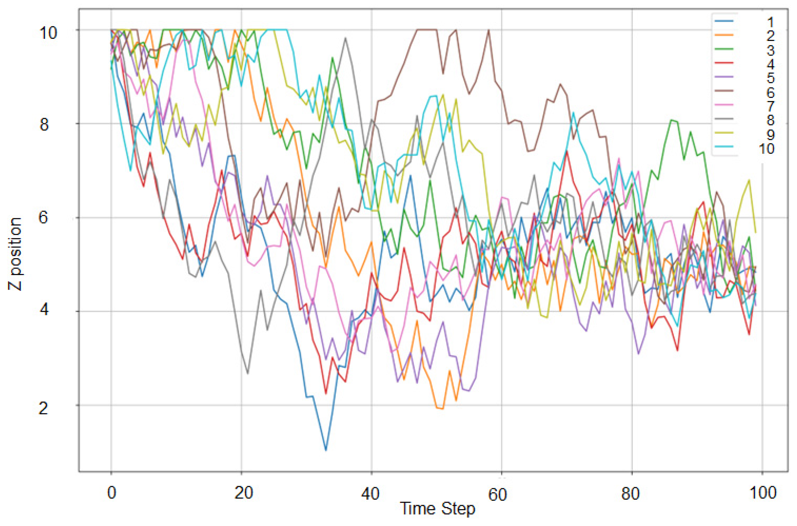
• Step 1. Data Preprocessing: The position data of the individuals that comprise the fish shoal are acquired and the position information for each time step is extracted.
• Step 2. Data Discretization: Divide the entire space over which the fishes can move into a mesh grid. This grid serves as a spatial unit for dividing the space into smaller cells.
• Step 3. Calculation of Fish Presence Probability in Each Cell at Each Timestep: For each timestep, calculate the probability of fish presence in each cell. This is achieved by counting the number of fish in the i-th cell and dividing by the total number of fish in the system at that time.

  $$p(x_i,t)=\frac{\mathrm{Number} \mathrm{of} \mathrm{fish} \mathrm{in} \mathrm{grid} i \mathrm{at} \mathrm{time} t}{\mathrm{Total} \mathrm{number} \mathrm{of} \mathrm{fish} \mathrm{at} \mathrm{time} t}$$

  (9)
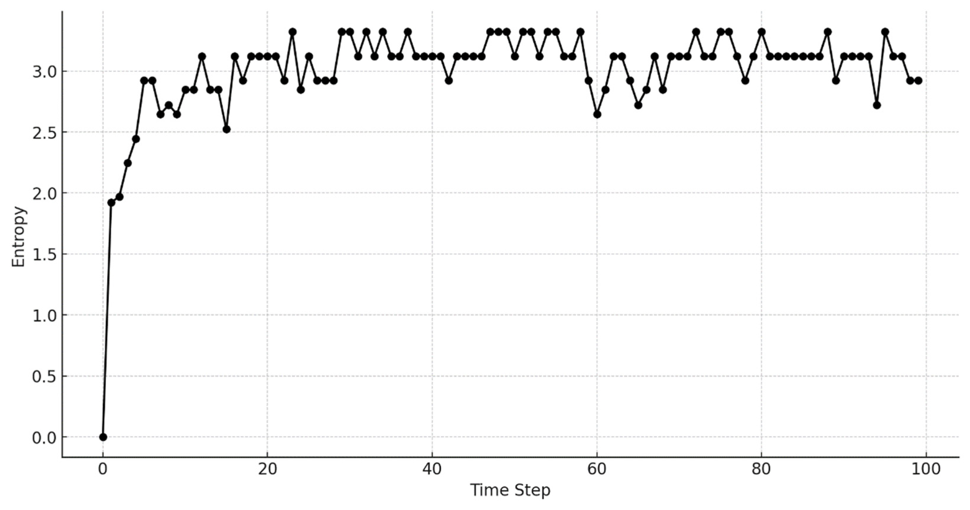
• Step 4. Calculation of Information Entropy at Each Timestep: Calculate the information entropy from the probability distribution $p(x_i,t)$ at each timestep. The information entropy $H\left(t\right)$ is calculated using the following formula:

  $$H\left(t\right)=-{{\displaystyle \sum }}_{i=1}^{n}p(x_i,t){\log }_{2}p(x_i,t)$$

  (10)

  where n is the total number of cells in the mesh grid, $p(x_i,t)$ is the probability of fish presence in the i-th cell at time t.
• Step 5. Plotting Information Entropy Over Time: Calculate the information entropy at each timestep and plot the changes in information entropy over time to visualize how the uncertainty and predictability of the data change over time.

In this paper, in order to create an appropriate dataset to perform this calculation directly, we first model the behavior of the fish population and calculate the information entropy for the results of the action trajectory simulation. Subsequently, we will describe the fish shoal behavior model.

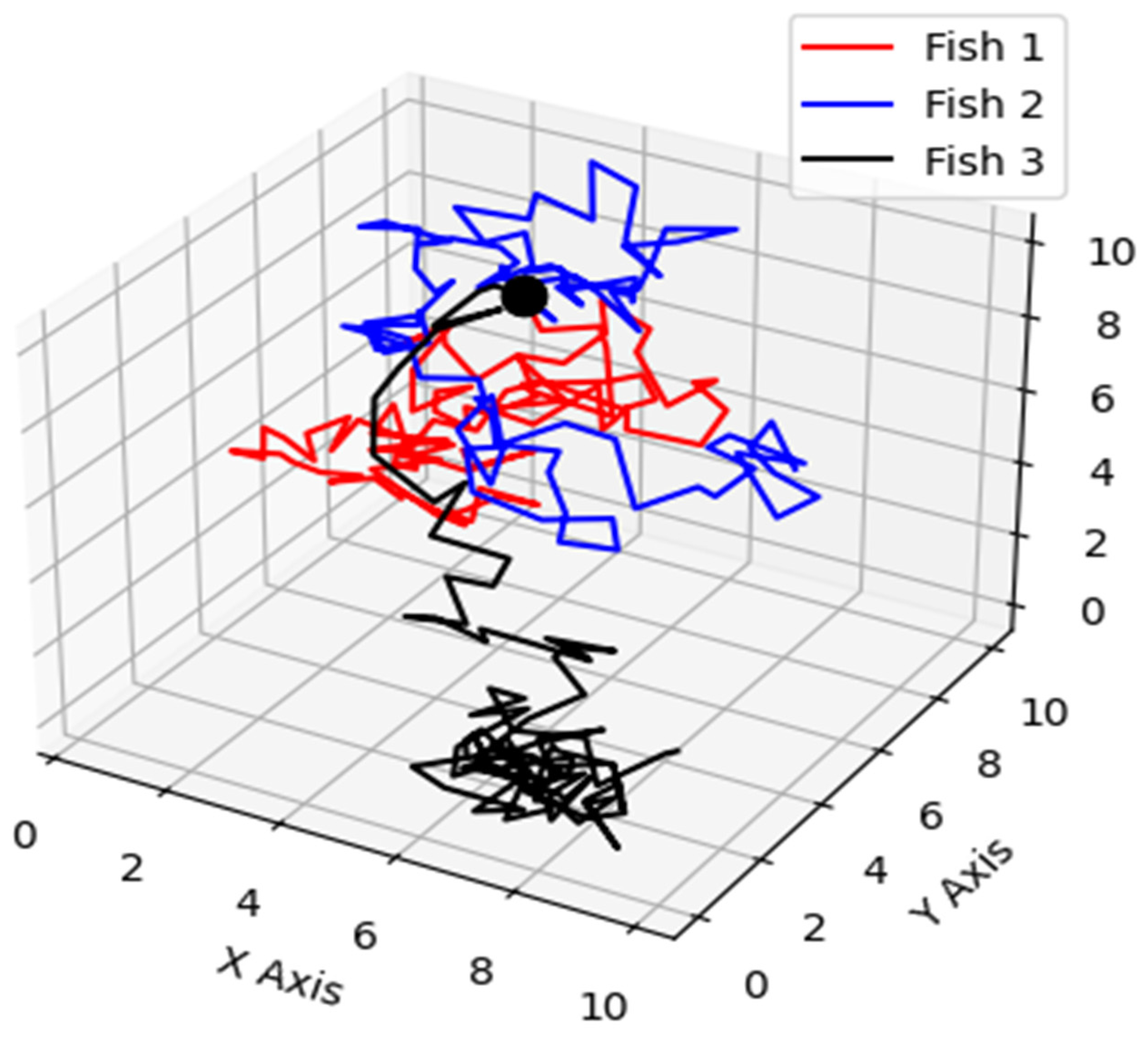
2.3. Fish Shoal Behavior Model

Research into fish movement has established that fish exhibit characteristics akin to a random walk—a pattern of movement inherently random in nature. For instance, organisms like Daphnia pulex and Temora longicornis have been observed performing multifractal random walks, behaviors linked to mating, foraging, and predator evasion strategies [24,25]. Moreover, studies have illustrated that movements within fish populations can be depicted through biased random walks, incorporating both directional movement and exploratory behavior [26]. These findings underscore the complexity of fish movements, rooted in the principles of random walks. In this study, we conceptualize the behavior of fish within a closed system as a random walk and proceed to simulate fish shoal behavior based on this model. The assumptions underlying the simulation model are detailed below.

Condition 1:

Fish move randomly within the system, with their next position dependent only on their current position, not on previous positions or movements.

Condition 2:

The system is composed of a three-dimensional space, assumed to be $0\le x\le 10.0\le y\le 10.0\le z\le 10$. These x, y, and z distances are non-dimensionalized to simplify the simulation and analysis, making the results more generally applicable and comparable across different scales and scenarios.

Condition 3:

Fish are simultaneously released from $x=5, y=5, z=10$.

Condition 4:

Upon reaching the system’s walls, fish are unable to continue in the same direction.

Condition 5:

Fish move to avoid collisions with each other. This is implemented by checking the presence of other fish in adjacent cells and adjusting the direction of movement to avoid these cells.

Condition 6:

There are 10 fish swimming within the system. The step length is fixed, and the direction of movement at each time step is chosen randomly by selecting a random angle in three-dimensional space.

We conducted 100 realizations of the simulations to ensure robustness and reproducibility of our results. Additionally, we will make our simulation codes publicly available on a repository such as GitHub to help readers understand the simulations better and reproduce our results.

Under these conditions, the calculated simulation results are shown in Figure 1. Three fish (Fish 1, Fish 2, Fish 3) were selected from the ten fish, and their trajectories were plotted in the 3D space with lines of different colors (red line, blue line, black line). The simulation calculated the movement of the fish over 100 time steps.

The random movements exhibited by fish are believed to be advantageous for predator evasion and adaptation to environmental variations. However, it is important to note that not all predator avoidance strategies are equally effective in all contexts. For instance, ballistic movements, which involve moving in a persistent direction (e.g., away from a predator), have been suggested as a better strategy to avoid predators in certain situations [27]. Reports by Steckbauer et al. (2018) and Abe M. and Kasada M. (2020) support the idea that random movements can be an effective avoidance strategy [28,29]. Thus, while our results indicate that random movements are advantageous, it is essential to consider these findings within the broader spectrum of predator–prey interaction strategies. The results of this simulation are considered reflective of significant elements of fish behavior. Moreover, within the framework of condition five, the simulation outcomes illustrate the ability of fish to detect the presence of their peers and adjust their actions accordingly. This study demonstrates the potential of utilizing simulation models to replicate fish movement responses to environmental shifts and the application of information entropy as an analytical tool to assess the dynamics of fish behavior and their implications.

3. Results and Discussion

In our research, we apply the previously outlined behavioral model to conduct a sensitivity analysis of information entropy in relation to the model’s parameters.

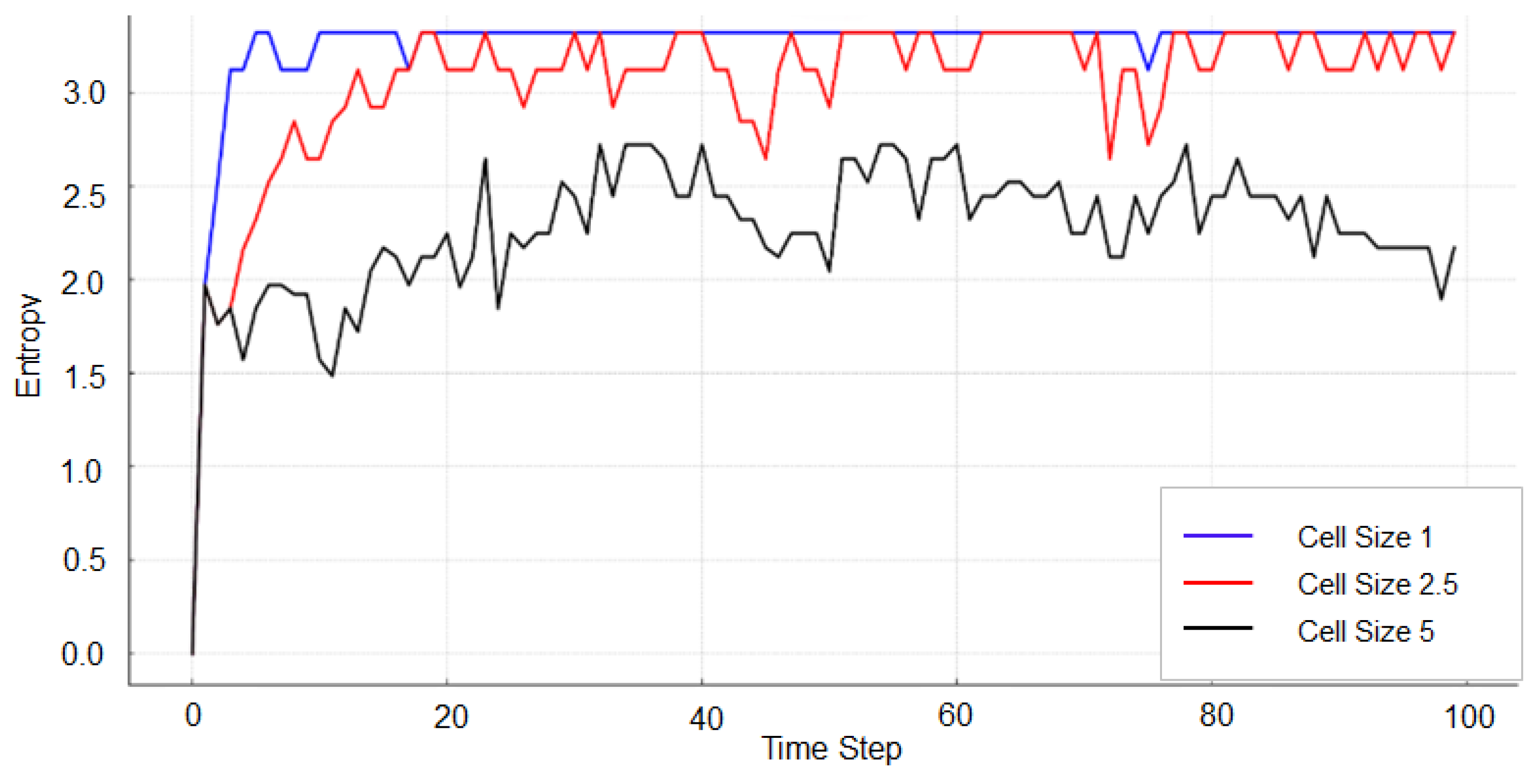
3.1. (Analysis-1) Selection of the Appropriate Cell Size

Analysis-1 focuses on determining the optimal cell size, which is crucial for the precise computation of entropy. Excessively large cells can obscure the true diversity in data distribution, resulting in an underestimation of the system’s inherent uncertainty and randomness. Conversely, cells that are too small may mistake mere noise for meaningful variations. Hence, selecting a cell size that aligns with the data’s characteristics and the analytical objectives is imperative to prevent inaccurate conclusions or information loss. To address this, we calculate information entropy using different grid dimensions (1, 2.5, 5) and conduct experiments to determine the “optimal” grid size that both meets our analytical goals and honors the inherent properties of the data. The experiments were designed to identify the “optimal” grid size by calculating entropy for varying cell dimensions within the simulation environment. Figure 2 illustrates the comparative entropy levels across 100 time steps for three different grid sizes. While this result is based on a single realization of the random walk model, it effectively demonstrates the impact of different cell sizes on entropy calculations. The consistency and reliability of the entropy calculations across different cell sizes validate the use of a single realization. Future studies will include multiple realizations to further enhance the robustness of the findings. The results indicate that the 1 × 1 × 1 cell size, represented by a blue line, generally exhibits higher entropy compared to larger cell sizes, suggesting that smaller cells are more sensitive to local variations, thus reflecting a higher resolution of information. However, the entropy for the 1 × 1 × 1 grid size does not show frequent fluctuations but maintains a consistently elevated level when compared to larger cell sizes. In contrast, data for the 5 × 5 × 5 cell size, depicted by a black line, shows significant fluctuations and appears less stable. This suggests that, in this particular case, larger cell sizes may not effectively smooth out minor data fluctuations and may still capture a certain level of variability.

The intermediate cell dimensions of 2.5 × 2.5 × 2.5, indicated by a red line, result in entropy values that fall between the smallest and largest cell sizes. This suggests that a cell size of 2.5 offers a balance, effectively capturing both granular details and broader patterns. These insights highlight that while smaller cell sizes can detect localized variability and intricate details, larger cell sizes are better suited for identifying widespread trends. Therefore, a cell size of 2.5 has been adopted for further analysis in this study, representing a compromise that emphasizes the importance of proper cell size selection in data analysis.

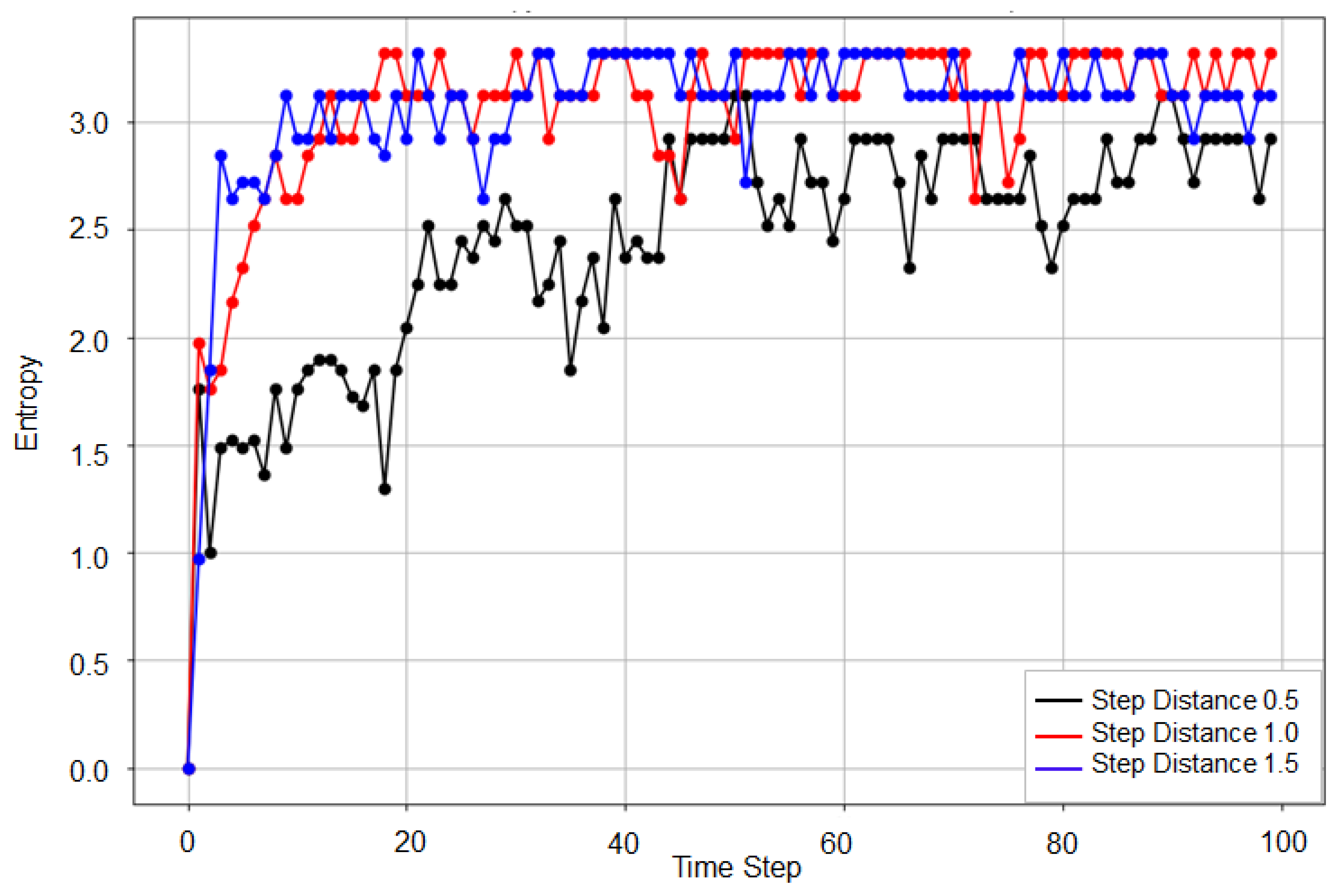
3.2. (Analysis-2) Sensitivity Analysis on Swimming Speed

This section of our Analysis delves into the effect of fish swimming speed variability on information entropy. We examine how altered swimming speeds, especially under stress conditions such as predatory threats or unfavorable environmental elements, influence the entropy metric. The study scrutinizes entropy variations across three distinct swimming speeds: 0.5, 1, and 1.5 per time step. This thorough investigation aims to yield quantitative insights into the impact of swimming speed on information entropy, thus shedding light on the significance of locomotion velocity in shaping the behavioral patterns of fish shoals and contributing to our understanding of ecological and ethological dynamics. Figure 3 offers a graphical comparison of entropy over 100 time steps for different step distances within a confined environment. The blue line represents the entropy at a step distance of 1.5, showing variable values that reflect a moderate sensitivity to changes in fish movement speed. The red line, illustrating a step distance of 1, consistently indicates higher entropy levels, implying a more scattered distribution of fish and greater uncertainty in their positioning. The black line, denoting a step distance of 0.5, displays comparatively lower and more stable entropy, suggesting a more aggregated distribution and more predictable movements within the system. The trends depicted in Figure 3 suggest that increased speed correlates with elevated entropy, indicative of swifter fish movements leading to a more dispersed distribution and, consequently, higher positional uncertainty within the confined space. Additionally, the figure correlates increased speeds with a rise in random movements and the emergence of unpredictable behavioral patterns, potentially resulting in an even distribution of fish throughout the system and amplified overall entropy. In contrast, slower speeds, as also depicted in the figure, tend to restrict fish movements and result in their concentration in specific areas, which may facilitate clustering. As shown in Figure 3, such constricted movement patterns are likely to increase the chances of fish aggregation in certain zones, corresponding to reduced entropy.

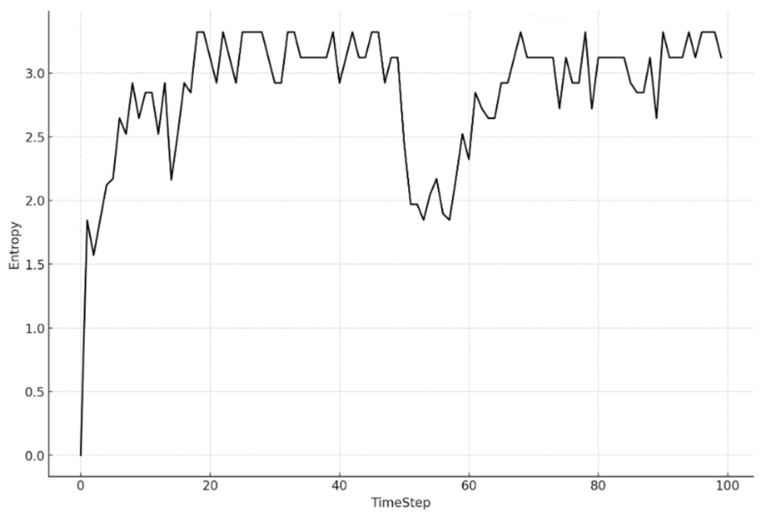
3.3. (Analysis-3) Behavioral Changes during Feeding and Entropy

The objective of this analysis is to ascertain whether fish feeding behavior patterns can be quantitatively evaluated using information entropy. For this purpose, we simulated the behavior of fish during feeding within our model. It is well-documented that certain species, such as tuna, exhibit phototaxis, actively avoiding light by diving deeper, a behavior that has significant implications for their feeding patterns [30]. Typically, in a fish pen, when feed is introduced, fish converge around the area where the food is distributed, begin feeding, and subsequently resume random swimming within the pen. In our simulation, this behavior is replicated at a specific moment (time step 50), where all fish are relocated to the vicinity of the water surface’s center, signifying the act of feeding. The simulation depicts both this feeding action and the subsequent random swimming. Through the simulation results, we scrutinize the fish’s feeding behavior patterns by examining entropy to determine if we can quantitatively capture the variability and irregularity of their behavior. Figure 4 graphically illustrates the entropy variation over time, showcasing the effect of a simulated feeding event on a shoal of fish within a controlled system. A significant drop in entropy at time step 50 corresponds to the feeding introduction, causing fish to cluster at a designated location, thus diminishing the randomness of their distribution. To evaluate entropy’s effectiveness in capturing changes in fish behavior during feeding events, we incorporated a simulated feeding event described above at time step 50 into the model and analyzed the ensuing data. Figure 4 indicates a notable decrease in entropy at this juncture, underscoring that upon feeding, the fish tend to gather at a certain location, transiently focusing the shoal’s distribution and consequently reducing the randomness of their behavioral pattern. Assuming the fish return to their initial random movements post-feeding, an escalation in entropy is anticipated. In accordance with this supposition, Figure 4 demonstrates that following the feeding event, entropy levels ascend as the fish disperse and revert to their prior movement patterns. The fleeting nature of the behavioral shift during feeding, followed by the reinstatement of the shoal’s original random movements, is effectively portrayed by the entropy fluctuations depicted in Figure 4.

This figure provides a graphical representation of the entropy variation over time, illustrating the impact of a simulated feeding event on the behavior of a fish shoal within a controlled system. The graph displays entropy values at each timestep, calculated with a logarithmic base 2 scale and distributed across 64 bins. A noticeable dip in entropy at timestep 50 corresponds to the introduction of food, which causes the fish to gather at a specific location, thereby reducing the randomness of their distribution. Following the feeding event, the entropy increases, suggesting a return to the initial random movement patterns. This figure effectively encapsulates the dynamism of fish behavior in response to feeding and the utility of entropy as a measure of such changes.

3.4. (Analysis-4) Behavioral Changes and Entropy in Response to External Stimuli

This analysis investigates the responsiveness of fish to external stimuli, particularly light, and whether this response can be quantified and evaluated using information entropy. A three-dimensional model was employed to simulate fish behavior in avoidance of light. From time step 50 onwards, zones of varying light intensities were established within the tank, and fish were programmed to favor dimmer areas. More specifically, when fish were situated in brighter areas (above 5 vertically), the likelihood of them moving downwards (in the negative Z-axis direction) was heightened, and conversely, when they were in darker areas (below 5 vertically), the probability of them moving upwards (in the positive Z-axis direction) was reduced. This method enabled us to simulate and analyze changes in fish behavior in response to light as an external stimulus through entropy. Following time step 50, the model introduced additional behavioral directives for the fish, particularly regarding their movement along the Z-axis. Fish located above 5 were more prone to descend, whereas those below 5 were less likely to ascend, resulting in a marked tendency for the fish to move toward the bottom. Figure 5 illustrates the depth (Z position) of each fish from the onset of the simulation, with each line in the graph detailing the temporal changes in depth for each fish, accentuating the behavioral shifts subsequent to time step 50. As Figure 6 reveals, the information entropy variations following time step 50 are not adequately explained by the entropy graph in isolation. To delineate the entropy fluctuation patterns with greater precision, we employed a Gaussian mixture model (GMM)—a method proven effective in previous studies for analyzing complex data distributions [31,32]. By clustering the time series entropy data into three distinct groups using GMM, we could identify nuanced behavior patterns within the data. The clustering outcomes, demonstrated in Figure 7, are consistent with established methodologies and reinforce the interpretive strength of GMM in the statistical analysis of ecological data. The characteristics of each cluster are as follows: Cluster 1 (blue) captures the early phase of the simulation, marked by the fish’s random movement, as reflected in the entropy fluctuations. Cluster 2 (red) represents an intermediate stage, where the fish have adjusted to the system and exhibit random yet patterned movements, potentially to circumvent obstacles and other fish. Cluster 3 (green) denotes the period post time step 50 where new behavioral rules have been implemented, capturing the fish’s adaptation to environmental changes such as light variation, which is paralleled by shifts in entropy. Thus, through the estimation of entropy, it is possible to highlight temporal changes in the directionality of the behavior characterized by a fish shoal from the distribution location of fish behavior.

4. Conclusions

In this paper, we quantitatively evaluate the complexity and predictability of fish shoal behavior in a closed system using information entropy. We highlight the significance of information entropy as an indicator for swimming patterns, feeding behavior, and responses to external stimuli in fish. Our initial examination focused on selecting an appropriate cell size for calculating entropy. Analysis of different cell sizes (1, 2.5, 5) revealed that smaller cells capture local fluctuations and fine details, while larger cells represent general trends. We determined that a 2.5 grid size optimally balances these considerations, enhancing the accuracy of modeling fish movements.

Our sensitivity analysis shows that higher swimming speeds correlate with increased entropy, indicating that faster-moving fish are more dispersed, increasing positional uncertainty. Conversely, slower-moving fish concentrate in specific areas, resulting in lower entropy. During feeding, entropy significantly decreased as fish congregated, followed by a return to original movement patterns.

Visualizing fish responses to external stimuli (such as light) using entropy was challenging due to the complexity of their behavior. However, applying the Gaussian mixture model (GMM) clarified the impact of environmental factors on entropy fluctuations. The GMM revealed distinct entropy clusters corresponding to different environmental influences, especially after time step 50, where changes in vertical light intensity showed distinct entropy patterns. These insights suggest the necessity of examining biological and environmental factors underlying entropy fluctuations.

Our results confirm the effectiveness of information entropy in evaluating fish shoal behavior complexity and predictability. This study’s significance lies in ecological and environmental management, providing a new method for analyzing fish behavior in natural settings and understanding biological responses to environmental changes. Future research will incorporate spatial variations in information entropy to capture more detailed patterns within fish shoals, refining this method for understanding collective behavior.

Overall, this research offers a fresh methodology for understanding collective fish behavior with potential applications in ecological studies and environmental management.

References

1. Zheng, M.; Kashimori, Y.; Hoshino, O.; Fujita, K.; Kambara, T. Behavior pattern (innate action) of individuals in fish schools generating efficient collective evasion from predation. J. Theor. Biol. 2005, 235, 153–167. [Google Scholar] [CrossRef] [PubMed]
2. Gazzola, M.; Tchieu, A.; Alexeev, D.; Brauer, A.; Koumoutsakos, P. Learning to school in the presence of hydrodynamic interactions. J. Fluid Mech. 2015, 789, 726–749. [Google Scholar] [CrossRef]
3. Thilsted, S.; Thorne-Lyman, A.; Webb, P.; Bogard, J.; Subasinghe, R.; Phillips, M.; Allison, E. Sustaining healthy diets: The role of capture fisheries and aquaculture for improving nutrition in the post-2015 era. Food Policy 2016, 61, 126–131. [Google Scholar] [CrossRef]
4. Embling, C.; Sharples, J.; Armstrong, E.; Palmer, M.; Scott, B. Fish behaviour in response to tidal variability and internal waves over a shelf sea bank. Prog. Oceanogr. 2013, 117, 106–117. [Google Scholar] [CrossRef]
5. Stöcker, S. Models for tuna school formation. Math. Biosci. 1999, 156, 167–190. [Google Scholar] [CrossRef]
6. Gebremedhin, S.; Bruneel, S.; Getahun, A.; Anteneh, W.; Goethals, P. Scientific Methods to Understand Fish Population Dynamics and Support Sustainable Fisheries Management. Water 2021, 13, 574. [Google Scholar] [CrossRef]
7. Partridge, B.L. The structure and function of fish schools. Sci. Am. 1982, 246, 114–123. [Google Scholar] [CrossRef]
8. Suzuki, K.; Torisawa, S.; Takagi, T. Mathematical and Experimental Analysis of Schooling Behavior During Growth in Juvenile Chub Mackerel: Considerations of Population Density and Space Limitation. In Proceedings of the ASME 2007 26th International Conference on Offshore Mechanics and Arctic Engineering, San Diego, CA, USA, 10 June 2007. [Google Scholar] [CrossRef]
9. Killen, S.; Marras, S.; Steffensen, J.; McKenzie, D. Aerobic capacity influences the spatial position of individuals within fish schools. Proc. R. Soc. B Biol. Sci. 2012, 279, 357–364. [Google Scholar] [CrossRef]
10. Weihs, D. Hydromechanics of Fish Schooling. Nature 1973, 241, 290–291. [Google Scholar] [CrossRef]
11. Aoki, I. A simulation study on the schooling mechanism in fish. Nippon. Suisan Gakkaishi 1982, 48, 1081–1088. [Google Scholar] [CrossRef]
12. Reynolds, C.W. Flocks, herds and schools: A distributed behavioral model. In Proceedings of the 14th Annual Conference on Computer Graphics and Interactive Techniques, Anaheim, CA, USA, 27–31 July 1987; pp. 25–34. [Google Scholar]
13. Bhooshan, N. The Simulation of the Movement of Fish Schools; Undergraduate Report; Institute of Systems Research University of Maryland: College Park, MD, USA, 3 August 2000. [Google Scholar]
14. Saila, S.B. Ecosystem Models of Fishing Effects: Present Status and a Suggested Future Paradigm. In The Future of Fisheries Science in North America; Beamish, R.J., Rothschild, B.J., Eds.; Fish & Fisheries Series; Springer: Dordrecht, The Netherlands, 2009; Volume 31, pp. 245–253. [Google Scholar] [CrossRef]
15. Gyllingberg, L.; Birhane, A.; Sumpter, D.J. The lost art of mathematical modelling. Math. Biosci. 2023, 362, 109033. [Google Scholar] [CrossRef] [PubMed]
16. Shannon, C.E.; Weaver, W. The Mathematical Theory of Communication; University of Illinois Press: Urbana, IL, USA, 1964; pp. 3–115. [Google Scholar]
17. Jiang, F.; Sui, Y.; Cao, C. An information entropy-based approach to outlier detection in rough sets. Expert Syst. Appl. 2010, 37, 6338–6344. [Google Scholar] [CrossRef]
18. Zhangchun, T.; Zhenzhou, L.; Biao, J.; Wang, P.; Feng, Z. Entropy-Based Importance Measure for Uncertain Model Inputs. AIAA J. 2013, 51, 2319–2334. [Google Scholar] [CrossRef]
19. Gong, W.; Yang, D.; Gupta, H.; Nearing, G. Estimating information entropy for hydrological data: One-dimensional case. Water Resour. Res. 2014, 50, 5003–5018. [Google Scholar] [CrossRef]
20. Ulanowlcz, R.; Norden, J. Symmetrical overhead in flow networks. Int. J. Syst. Sci. 1990, 21, 429–437. [Google Scholar] [CrossRef]
21. Pennekamp, F.; Iles, A.; Garland, J.; Brennan, G.; Brose, U.; Gaedke, U.; Jacob, U.; Kratina, P.; Matthews, B.; Munch, S.; et al. The intrinsic predictability of ecological time series and its potential to guide forecasting. bioRxiv 2018. [Google Scholar] [CrossRef]
22. Majerník, V. Entropy—A Universal Concept in Sciences. Nat. Sci. 2014, 6, 552–564. [Google Scholar] [CrossRef]
23. Kala, Z. Quantification of Model Uncertainty Based on Variance and Entropy of Bernoulli Distribution. Mathematics 2022, 10, 3980. [Google Scholar] [CrossRef]
24. Seuront, L.; Schmitt, F.; Brewer, M.; Strickler, J.; Souissi, S. From random walk to multifractal random walk in zooplankton swimming behavior. Zool. Stud. 2004, 43, 498–510. [Google Scholar]
25. Faugeras, B.; Maury, O. Modeling fish population movements: From an individual-based representation to an advection-diffusion equation. J. Theor. Biol. 2007, 247, 837–848. [Google Scholar] [CrossRef]
26. Kadota, M.; Torisawa, S.; Tsutomu, T.; Komeyama, K.; Fukuda, H. Analysis of juvenile tuna movements as correlated random walk. Fish. Sci. 2011, 77, 993–998. [Google Scholar] [CrossRef]
27. Pagès, J.; Bartumeus, F.; Romero, J.; Alcoverro, T. The scent of fear makes sea urchins go ballistic. Mov. Ecol. 2021, 9, 50. [Google Scholar] [CrossRef] [PubMed]
28. Steckbauer, A.; Díaz-Gil, C.; Alós, J.; Catalán, I.; Duarte, M. Predator Avoidance in the European Seabass After Recovery From Short-Term Hypoxia and Different CO2 Conditions. Front. Mar. Sci. 2018, 5, 350. [Google Scholar] [CrossRef]
29. Abe, M.; Kasada, M. Optimal Random Avoidance Strategy in Prey-Predator Interactions. bioRxiv 2020, 2020.03.04.976076. [Google Scholar] [CrossRef]
30. Nuno, A.; Guiet, J.; Baranek, B.; Bianchi, D. Patterns and drivers of the diving behavior of large pelagic predators. bioRxiv 2022, 12.27.521953. [Google Scholar] [CrossRef]
31. Morad, N. Modeling Methods in Clustering Analysis for Time Series Data. Open J. Stat. 2020, 10, 565–580. [Google Scholar] [CrossRef]
32. McDowell, I.; Manandhar, D.; Vockley, C.; Schmid, A.; Reddy, T.; Engelhardt, B. Clustering gene expression time series data using an infinite Gaussian process mixture model. PLoS Comput. Biol. 2018, 14, e1005896. [Google Scholar] [CrossRef]
Figure 1. Three-dimensional trajectories of three fish in closed system. This figure represents the simulation results of fish movement within a confined space. From the ten fish in the simulation, three (Fish 1, Fish 2, and Fish 3) were selected, and their paths are depicted in the 3D space with lines of different colors (red for Fish 1, blue for Fish 2, and black for Fish 3). The simulation tracked the movement of these fish over the course of 100 time steps, showcasing the variability in their behavior under the defined simulation conditions. The central black dot indicates the starting point at T = 0.
Fishes 09 00224 g001
Figure 2. Entropy over time for different cell sizes. This figure illustrates the comparative entropy levels over 100 time steps for three different grid sizes within the simulation environment. The blue line represents the entropy for a 1 × 1 × 1 cell size, displaying consistently higher values, which suggests a heightened sensitivity to localized data variation. The black line depicts the entropy for a 5 × 5 × 5 cell size, which is notably the lowest and most stable across the time steps, indicating a smoothing of finer data fluctuations and a capture of more general trends. The red line corresponds to the intermediate 2.5 × 2.5 × 2.5 cell size, with entropy levels falling between those of the smallest and largest cell sizes, pointing to an effective balance between detail capture and trend representation. The entropy trends observed for each cell size illustrate the implications of grid dimension choice on the resolution of information extracted from the data. The cell size of 2.5 × 2.5 × 2.5 was subsequently adopted for further analysis within this study due to its balanced approach.
Fishes 09 00224 g002
Figure 3. Entropy comparison for different step distances. This figure provides a visual comparison of entropy over 100 time steps for fish exhibiting different step distances within a confined system. The blue line represents the entropy for a step distance of 1.5, showing fluctuating values that suggest moderate sensitivity to the speed of fish movement. The red line, representing a step distance of 1.0, generally indicates higher entropy, denoting a more dispersed fish distribution and higher uncertainty in their positions. Lastly, the black line illustrates the entropy for a step distance of 0.5, which remains relatively lower and more stable, implying a less dispersed distribution and a tendency towards more predictable movement patterns within the system.
Fishes 09 00224 g003
Figure 4. Entropy over time during feeding events.
Fishes 09 00224 g004
Figure 5. Vertical position over time for each fish. This figure shows the vertical trajectories of ten fish throughout the simulation, with each line tracing a distinct fish’s movement in water depth from the outset. Post time step 50, noticeable shifts in these trajectories suggest behavioral adjustments among the fish.
Fishes 09 00224 g005
Figure 6. Information entropy over time steps. This figure captures the vertical trajectories of ten fish throughout the simulation, with each line tracing a distinct fish’s movement in water depth from the outset. Post time step 50, noticeable shifts in these trajectories suggest behavioral adjustments among the fish.
Fishes 09 00224 g006
Figure 7. Gaussian mixture model clustering of time steps in entropy data. This figure displays the result of employing a Gaussian mixture model (GMM) for categorizing the information entropy time series into three distinct clusters. Cluster 1 (blue) indicates the simulation’s early phase, marked by erratic fish motion and entropy swings. Cluster 2 (red) shows a more stable phase as fish adjust to their environment, adopting random but systematic movement patterns, such as avoiding obstacles. Cluster 3 (green) represents the phase after introducing new behavior rules at time step 50, capturing the fish’s adaptive response to environmental changes, as reflected by the shifts in entropy.
Fishes 09 00224 g007
Disclaimer/Publisher’s Note: The statements, opinions and data contained in all publications are solely those of the individual author(s) and contributor(s) and not of MDPI and/or the editor(s). MDPI and/or the editor(s) disclaim responsibility for any injury to people or property resulting from any ideas, methods, instructions or products referred to in the content.