Article

A Study on the Impact of Environmental Factors on Chub Mackerel Scomber japonicus Fishing Grounds Based on a Linear Mixed Model

1
Key and Open Laboratory of Remote Sensing Information Technology in Fishing Resource, East China Sea Fisheries Research Institute, Chinese Academy of Fishery Sciences, Shanghai 200090, China
2
College of Fisheries and Life Science, Shanghai Ocean University, Shanghai 201306, China
*
Author to whom correspondence should be addressed.
Fishes 2024, 9(8), 323; https://doi.org/10.3390/fishes9080323
Submission received: 14 June 2024 / Revised: 25 July 2024 / Accepted: 9 August 2024 / Published: 14 August 2024
(This article belongs to the Special Issue Biodiversity and Spatial Distribution of Fishes)

Abstract

:
Chub mackerel (Scomber japonicus) is a commercially important fish species which are widely distributed in the North Pacific. Based on the fishery data from China’s high-sea light-purse seine fishing from 2014 to 2020 and the marine environment factors, a mixed linear model considering the actual spatiotemporal stratification of the catch per unit effort (CPUE) was established to analyze the fixed and random effects of marine environmental factors on the CPUE of chub mackerel and to investigate the relationship between the abundance of chub mackerel resources in the Northwest Pacific and two marine environmental factors: sea surface temperature (SST) and chlorophyll-a concentration (CHL). The results showed that SST had a significant fixed effect on the CPUE. In contrast, the natural logarithm of chlorophyll (logCHL) had no fixed effect on the CPUE. Based on the monthly analysis, random fluctuations were observed in the impact of logCHL on the CPUE. LogCHL and CPUE show a positive correlation during spawning and wintering periods and a negative correlation during the feeding period. The study showed that when fishery sampling data exhibit spatiotemporal stratification, linear mixed models can effectively incorporate both the fixed and random effects of environmental factors on the CPUE of chub mackerel. Linear mixed models can play an important role in analyzing the fluctuations in resource abundance and the mechanisms governing the formation of fishing grounds for chub mackerel in the Northwest Pacific.
Key Contribution: A mixed linear model was introduced to analyze the fixed and random effects of marine environmental factors on CPUE of chub mackerel; SST had a significant fixed effect on CPUE, random fluctuations were observed in the impact of logCHL on CPUE.

1. Introduction

Chub mackerel is a small fish species which inhabit the upper and middle layers of subtropical to temperate waters and is widespread in the Indian Ocean, the Pacific coast of South America, and the Western Pacific [1,2,3]. Based on the migration patterns and spawning areas, chub mackerel in the Northwest Pacific can be divided into two stocks: the Tsushima Warm Current (TWC) stock, which is distributed in the East China Sea, the Yellow Sea, and the Sea of Japan, and the Pacific stock, which is distributed around the edge of the Kuroshio current [2,4]. Chub mackerel plays an important role in global fisheries, with its stock biomass and catch showing significant year-to-year fluctuations [5]. Chinese fishing vessels have been conducting purse seine fishing operations in the Northwest Pacific since 2014. Catches of chub mackerel peaked at 150,000 tonnes in 2015 and fell to 80,000 tonnes in 2020 [6].
Previous studies have suggested that the marine environment was closely related to the growth rate, distribution of resources, and changes in fishing grounds for chub mackerel. During their early life stages, the growth, migration, and recruitment of chub mackerel are influenced by both biological and abiotic factors [1,3,7,8,9]. Chub mackerel larvae can be transported to downstream areas of the Kuroshio–Oyashio Transition Area (KOTA) for feeding purposes. The KOTA is characterized by abundant bait resources and plays a role as an important habitat for several small pelagic fish species, including chub mackerel [1,7,10]. In the Northwest Pacific, the concentration of chlorophyll can serve as a reference indicator for the foraging of chub mackerel and can influence the aggregation of chub mackerel on a large scale, especially in the vicinity of the Kuroshio and Oyashio fronts [11,12]. In the southern waters of the East China Sea, the distribution of chub mackerel is influenced by the invasion of the warm Kuroshio current [13]. Sea surface temperature (SST) is considered to be an important environmental factor affecting the spawning and migration patterns of chub mackerel [4,14], as well as affecting the catch per unit effort (CPUE), which is used as an index of relative resource abundance [15,16]. For example, SST had a positive effect on the CPUE between 6 °C and 19 °C and a negative effect between 19 °C and 35 °C for the Korean large purse seine fishery [15]. Within the appropriate temperature and salinity range (suitable water temperature of 20 °C and suitable salinity of 33.75‰), chub mackerel tend to aggregate at the convergence zone between the cold and warm water masses, where significant thermal gradients and salinity gradients exist [17]. Furthermore, the fishing grounds for chub mackerel are affected by changes in the path of the Kuroshio current [17] and climatic regime shifts [18]
To better understand the relationship between the spatiotemporal distribution and resource abundance of chub mackerel and environmental factors, researchers have developed different models using different statistical or machine learning methods, such as GLM and GAM models [15,19,20], minimum volume ellipsoid [3], the habitat suitability index [21,22], and deep learning models [10,23]. These studies suggest that the spatiotemporal distribution of chub mackerel depends on environmental factors, including SST, chlorophyll-a concentration (CHL), sea surface height, and sea surface salinity. However, there exist some differences in the importance of various marine factors among different studies.
However, previous studies on the relationship between chub mackerel resource abundance and the marine environment usually did not take sufficient account of the differences among various spatiotemporal groups of fishery sample data. The age composition of chub mackerel always shows significant variability across different years [6], and the degree of influence of environmental factors on fish at different ages is often different [24,25]. This variability results in the year stratification of data. Furthermore, chub mackerel display obvious migratory behavior, leading to shifts in fishing areas across seasons. The water mass configuration in the fishing ground also varies across different zones and seasons. Consequently, the impact of marine environmental factors on mackerel fluctuates across different months or fishing zones, exhibiting certain patterns within the same month or fishing zone [11,26]. For fishery data with stratification, the different layers can be processed separately according to different months or fishing zones. However, the statistical significance of the results would be lost in a regression analysis due to the insufficient sample size. On the other hand, excessive data subsampling can lead to more complex data pre-processing and analysis as there is excessive stratification (such as an extensive division of fishing zones), which makes the application of the model difficult.
Some studies used a mixed-effects model to analyze the distribution of Georges Bank yellowtail flounder, and the results showed that the mixed-effects model was more parsimonious than the fixed effects model [27]. In this study, in order to enhance our understanding of the impact of marine environment changes on the distribution of mackerel under various spatiotemporal conditions, we analyze the fixed and random effects of SST and CHL on the CPUE of chub mackerel during various month and fishing zone stratifications through the mixed linear model, and investigate the effect of marine environmental changes on chub mackerel CPUE over time and space. Furthermore, this study aims to offer theoretical insights into the sustainable development and management of chub mackerel resources in the Northwest Pacific.

2. Materials and Methods

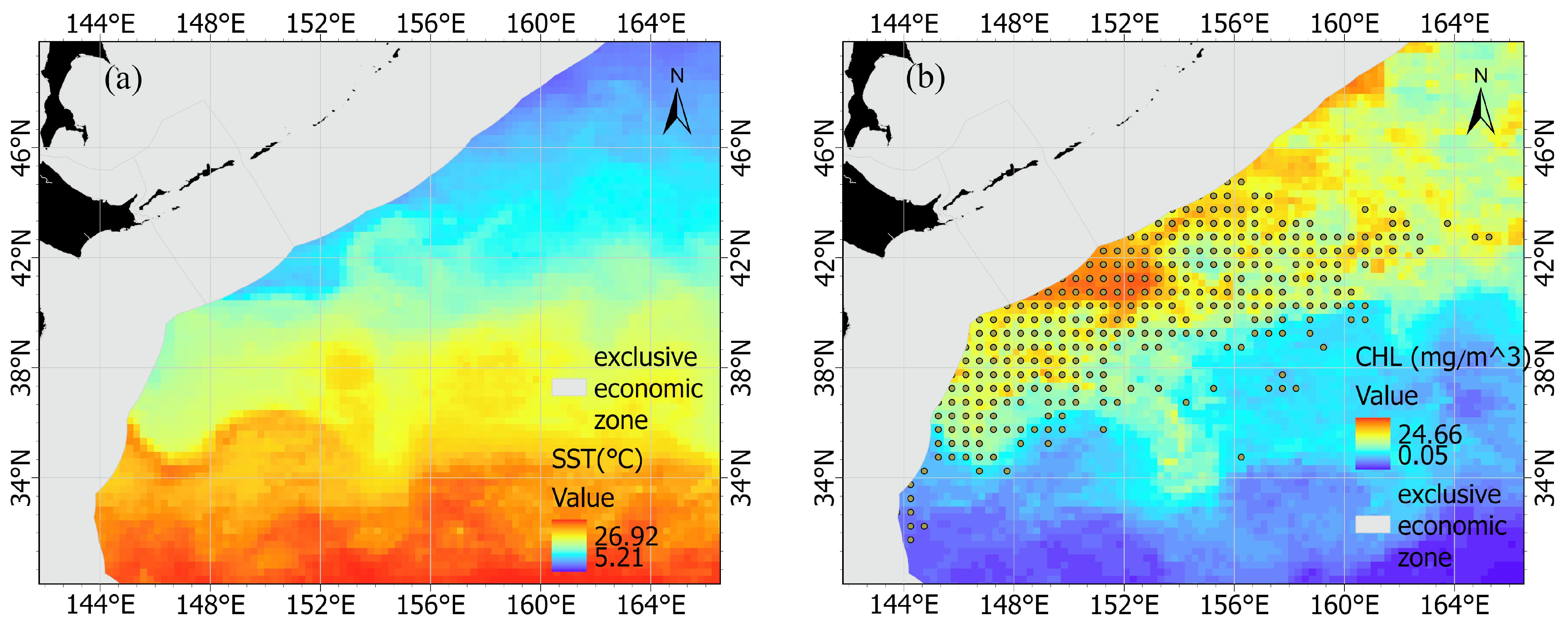
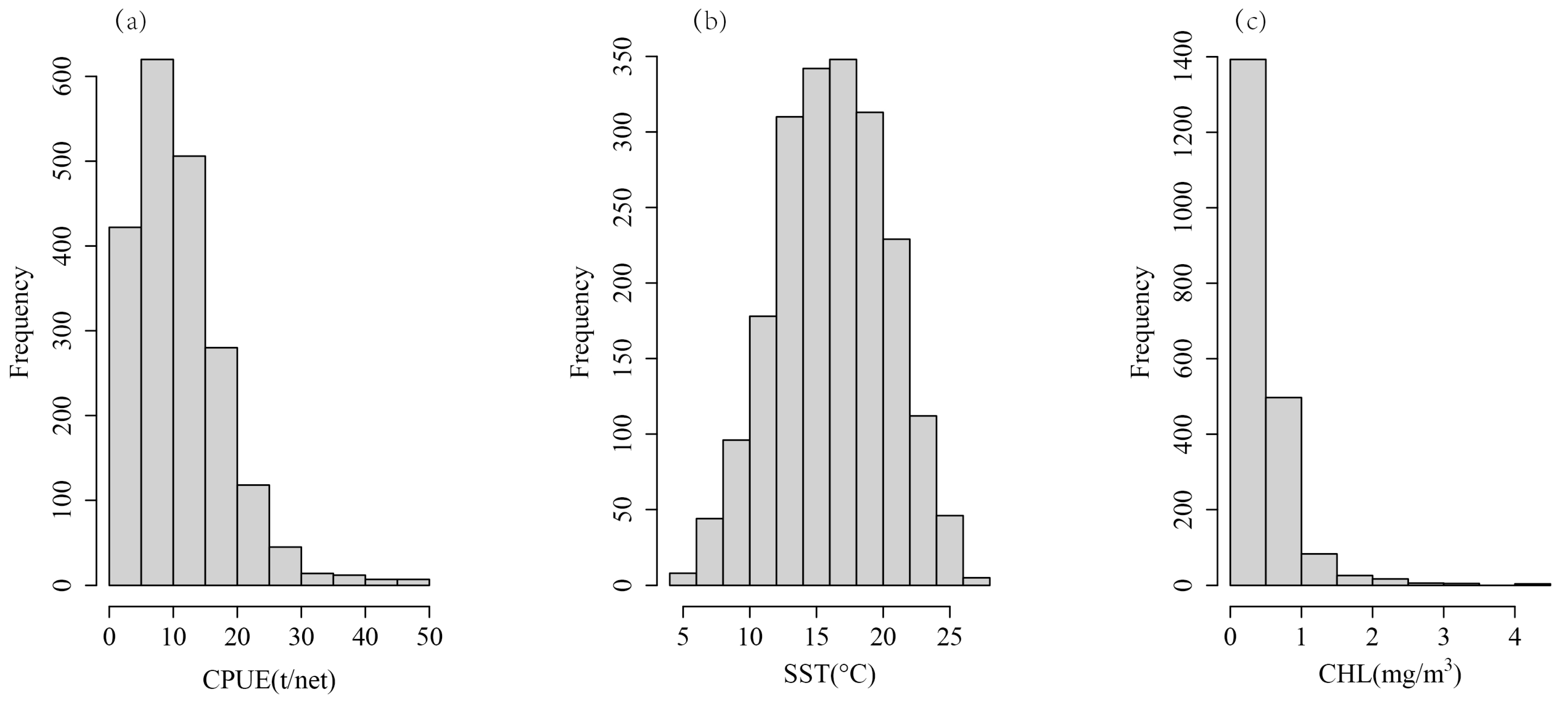
2.1. Environmental and Fishery Data

Previous studies demonstrated that SST (°C) and CHL (mg/m3) could have a significant impact on the catch and distribution of chub mackerel resources [3,9,11,28,29,30]. Therefore, SST and CHL were included in the model of the present study. The monthly averaged SST (Figure 1a) and the monthly averaged CHL (Figure 1b) were acquired from Oregon State University’s Ocean Productivity database (http://sites.science.oregonstate.edu/ocean.productivity/, accessed on 1 June 2022), and these data were resampled to a spatial resolution of 0.5° × 0.5°.
The fishing vessel production of China’s light-purse seine operations in the high seas of the Northwest Pacific from 2014 to 2020 was collected. The dataset includes the fishery operation dates, locations, net-haul numbers, catches, and so on. The study area covers the traditional fishing grounds of chub mackerel between 140–165° E and 30–50° N in the North Pacific. For each month, we aggregated the fishery data at a spatial resolution of 0.5° × 0.5°. The CPUE (t/net) was calculated with Equation (1).
CPUE = C / N
in which C is the total catch (t) in a single fishing zone, and N is the total number of nets hauled (net) in the same zone. To generate the dataset needed for modeling, CPUE was matched with environmental data by the month and zone.

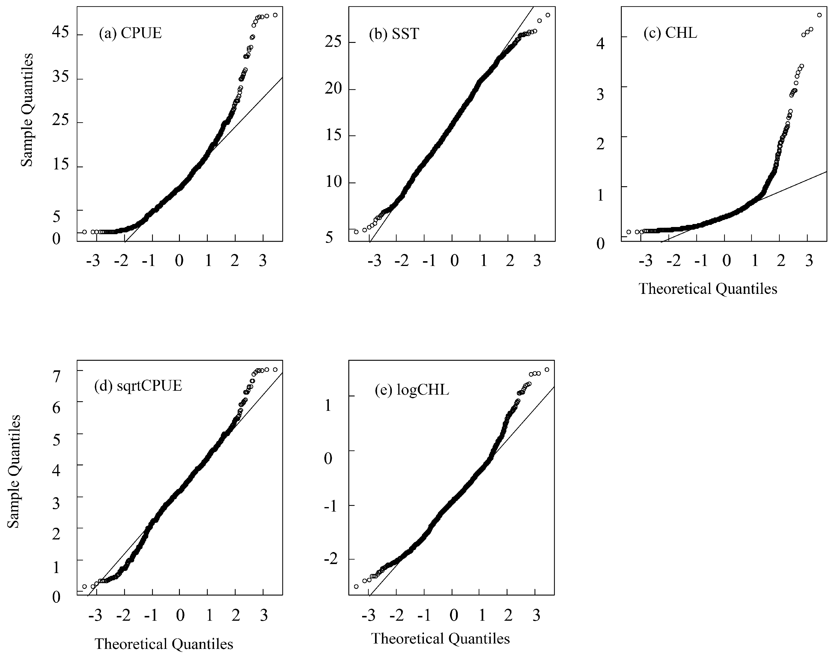
2.2. Normalization and Multicollinearity Detection of Variables

The distribution of CPUE, SST and CHL was shown in Figure 2. We tested the distribution of the CPUE, SST, and CHL to obtain skewness and kurtosis values. The results showed that, except for SST, the skewness of CPUE and CHL was much greater than 0, and the kurtosis was much greater than 3, which indicates a skewed distribution (Table 1, Figure 3). In order to obtain the normally distributed data, the CPUE, SST, and CHL were transformed by taking the natural logarithm or square root of each variable. The natural logarithm is also a method used when dealing with skew data in linear mixed-effects models [27]. The results indicated that the square root of the CPUE (denoted as sqrtCPUE) has a normal distribution (skewness closer to 0, kurtosis closer to 3), and the natural logarithm of CHL (denoted as logCHL) is normally distributed (as shown in Table 1 and Figure 3). The raw SST is close to a normal distribution, so the original SST is directly applied to the model (Table 1).
Variance inflation factors (VIF) were used to detect multicollinearity. The variance inflation factor (VIF) of SST and logCHL are both 1.990, which is below the threshold of 5, indicating the absence of multicollinearity between SST and logCHL [31].

2.3. Linear Mixed Model

Mixed-effects models incorporate both fixed effects and random effects [32]. The fixed effects in the model can effectively capture the overall trend of the dependent variable as it changes with the independent variable, while the random effects represent individual characteristics. Linear mixed models (LMMs) are flexible extensions of linear models which incorporate fixed and random effects [33]. Linear mixed-effects models can be mathematically manipulated as matrices as follows [34]:
Y = X β + Z u + ε
where Y = ( y 1 y 2 , , y N ) is the n × 1 vector of responses, and n = n 1 + n 2 + + n N . β is the p × 1 vector of fixed effects, X is the n × p design matrix for fixed effects, Z is the n × q 1 + q 2 + + q N matrix of random effects, b is the q 1 + q 2 + + q N × 1 vector, and ε is the n × 1 vector of errors, which captures the differences between the observed responses and the predicted responses based on the fixed and random effects in the model.
To determine the effects of SST and chlorophyll concentration on the different levels of CPUE, SST and logCHL were selected as possible fixed effects, and Year, Month, and fishing Zone were considered random effects. We used the lme4 package in the R environment to run the model [32,35]. The model Equation (2) can be written as follows [35]:
sqrtCPUE~1 + SST + logCHL + (1 + SST + logCHL|Year) + (1 + SST + logCHL|Month) + (1 + SST + logCHL|Zone)
in which variables without parentheses represent fixed effects, while Year, Month, and Zone in parentheses denote random effects. The variables to the left of the vertical line in parentheses are covariates; the constant value 1 represents the random intercept.

2.4. Selection of the Optimal Model

Initially, a null model can be developed by considering only the random intercepts, without factoring in the environmental variables. In simpler terms, Equation (3) can be expressed in the following manner:
SqrtCPUE~1 + (1|Year) + (1|Month) + (1|Zone)
By adding the SST and logCHL to the initial model, in fixed effect and random effect terms, 256 candidate models in all can be obtained. In order to choose the optimal model, we fit each candidate model to estimate the model parameters and performed significance tests on both fixed and random terms. Then, each model was assessed via information-based criteria such as AIC, BIC, log likelihood rate (logLik), and residuals. In addition, as strong correlations can affect the estimation of other covariate coefficients, the correlation between slopes and intercept within random effects was checked to ensure that the absolute values of the correlation coefficients between them were less than 0.7 [36,37,38].

3. Results

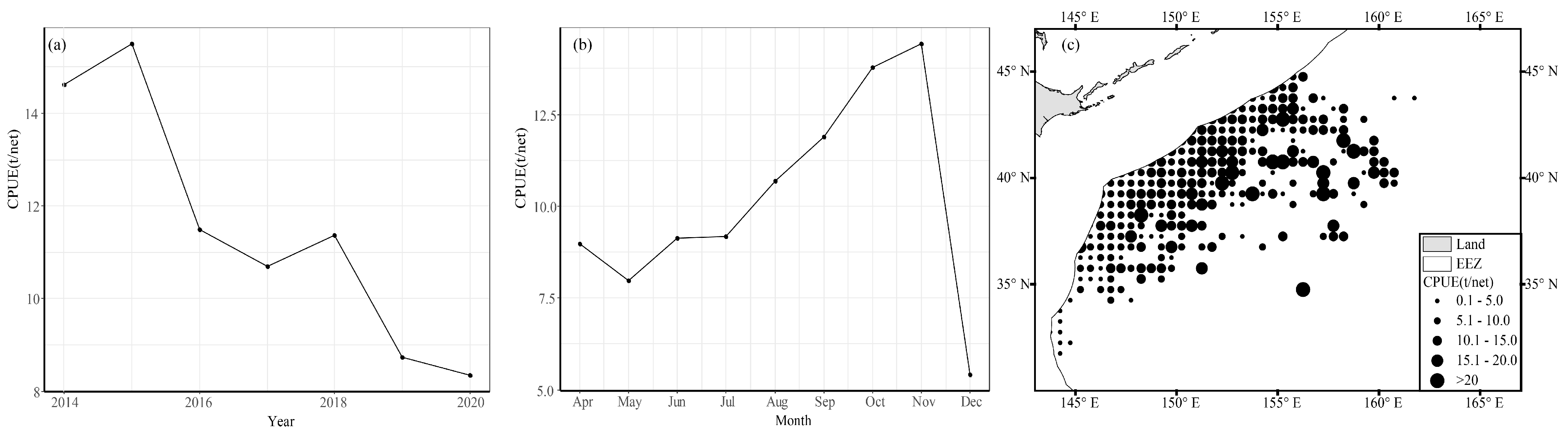
3.1. Seasonal Variation and Spatial Distribution of CPUE

The average annual CPUE of chub mackerel showed a trend of decreasing from 2014 to 2020. The CPUE peaked in 2015 and 2018 with values of 15.501 t/net and 11.363 t/net, respectively. In 2020, the CPUE reached its lowest point with a value of 8.355 t/net. In addition, the CPUE showed seasonal variations: The CPUE was relatively lower than 10 t/net from April to July. However, it increased rapidly after August and peaked in November with a value of 14.426 t/net, and then fell rapidly to 5.427 t/net in December.
On account of the spatial distribution patterns of fish, fishing areas with lower CPUE values (less than 5 t/net) were distributed in waters south of 34° N, while fishing areas with higher CPUE values (more than 15 t/net) were located between 148° and 159° E and were relatively dispersed.
As shown in Figure 4, the mean CPUE of chub mackerel varied significantly across different years, months, and spatial locations.

3.2. Optimal Linear Mixed Model

After calculating the AIC and other information-based criteria for a total of 256 candidate models, the models with fixed effect and random effect items that were statistically significant (p < 0.05) and the weak correlation (absolute value was less than 0.7) between the slope and intercept of random effect items were retained. As a result, six candidate models were finally obtained, as shown in Table 2. For comparison, the regression model with only fixed effects is also listed in the table, numbered 0.
As shown in Table 2, the values of AIC, BIC, and logLik in the scenario 0 model were relatively higher and did not show random effects. Among scenarios 1–6 with random effects, the scenario 5 model exhibited the highest accuracies with the lowest values of AIC, BIC, LogLik, and Deviance; thus, the scenario 5 model was selected as the optimal model, including SST as the fixed effect and three random effects. There was only a random intercept in the random effect zone; meanwhile, there were both an intercept and a slope of logCHL term in the random effect of Month.

3.3. Mixed Effects of SST and logCHL on CPUE

3.3.1. Fixed Effect Parameters

The optimal model (Model 5, Table 2) retained SST as a fixed effect. The intercept was positive, and the SST slope value was negative (Table 3). The t-test results for the intercept and slope indicated that both of them were statistically significant (p < 0.001).

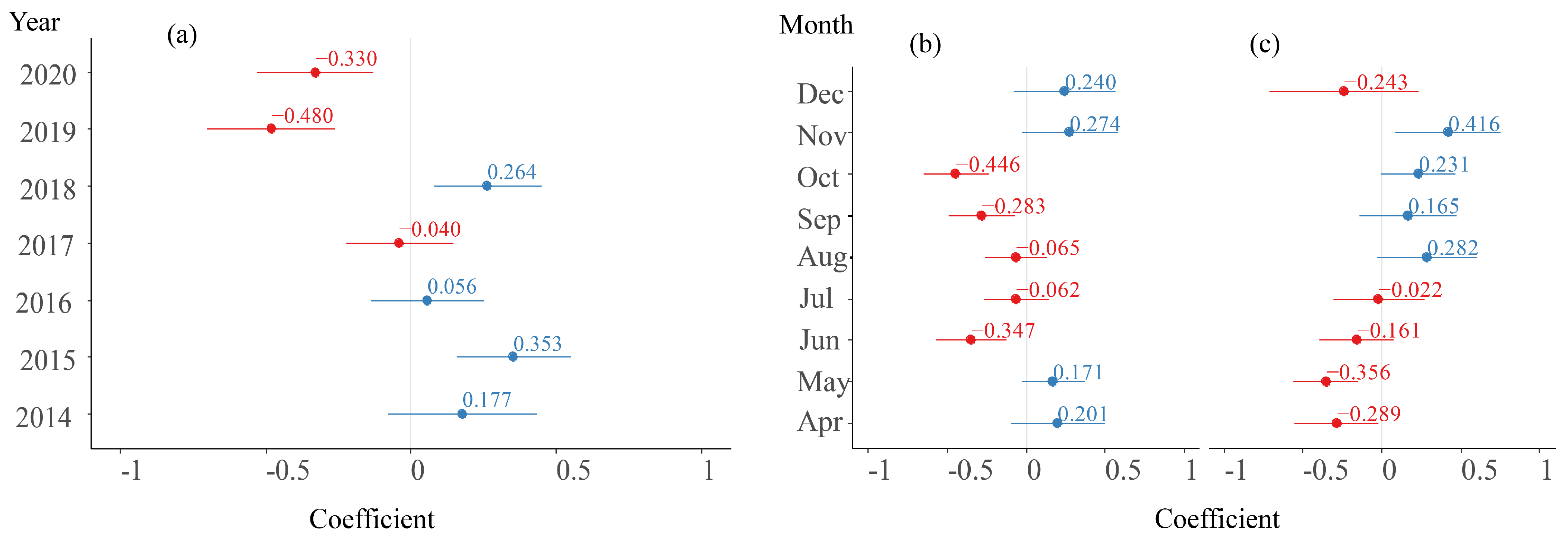
3.3.2. Random Effect Parameters

The variances and standard deviations (Std. Dev) of the random slope and random intercept coefficients in three random effects are shown in Table 4. In the Month group, the correlation coefficient between the random intercept and the slope of the covariate logCHL was −0.07, indicating a very weak correlation. This suggests that the estimation of model parameters was stable, with relatively low error and variability.
A likelihood ratio test (LRT) was also conducted on random effects. After removing three random effect terms, the accuracy of the model significantly decreased compared to that of the original model (p-values were all less than 0.05), suggesting that retaining the three random effect terms has great effects on the accuracy of the model (Table 5).
The average random intercept values for the Year group are shown in Figure 5a, with the highest value (0.353) observed in 2015 and the lowest value (−0.480) observed in 2019. Their trend over the years is consistent with the annual variation in the CPUE in Figure 4a. For the random effect of the Month, the fluctuation in the logCHL slope and intercept is shown in Figure 5b. The average slopes for April, May, November, and December are positive, while those from June to October are negative. In terms of the average intercept in the Month group, the values are positive from August to November, while they are negative for the remaining months, and the trend in the change is basically consistent with the monthly changes in the CPUE in Figure 4b.
As shown in Figure 6, the random intercept in the Zone group ranged between −0.164 and 0.260 with an average value of 0.000 ± 0.066. It is worth noting that there was a region located between 150–152° E and 39–41°, with relatively high slope values, which was very different from the high CPUE distribution in Figure 4c. The average slope value in the region was 0.098 ± 0.069.

3.4. Residual Test

One of the fundamental assumptions of mixed linear models is that the residuals are normally distributed. The skewness of residuals obtained in the present model was 0.031, which was close to 0 for the normal distribution. The kurtosis value was 3.532, which is close to 3 for the normal distribution. In addition, the points in the Quantile–Quantile Plot (Q-Q Plot) of the residuals were roughly distributed along a straight line (Figure 7). Therefore, it could be concluded that the residuals from the LMM closely approximate a normal distribution.

4. Discussion

4.1. Influence of SST on Chub Mackerel

The catch and biomass of chub mackerel are closely related to the recruitment stock population [4]. As a poikilotherm, the growth, mortality, and habitat selection of the chub mackerel are affected by seawater temperature and are highly sensitive to changes in seawater temperature [28,29,30,39]. The SST not only influences the growth rate of chub mackerel [5,7,40] but also has a great impact on the spatial distribution of chub mackerel. Previous studies have suggested that the optimal temperature for the fishing grounds of chub mackerel in the Northwest Pacific is between 14 and 18 °C, and larger catches are easily obtained in waters around 16 °C [11]. Within the appropriate temperature range, the catches will increase with higher water temperature and decrease with lower temperature [41]. However, some studies suggested that a lower SST often corresponds to a higher concentration of chub mackerel in fishing grounds in the East China Sea [9]. In the central Atlantic region of the Middle East, there is a significant negative correlation between chub mackerel catch and SST [42]. In the coastal sea around Japan, an increased SST can result in a decrease in stock size for chub mackerel [43]. Our study showed that the slope of SST in fixed effect exhibited a negative value (Table 3), which is consistent with the above mentioned studies [9,42,43]. It implies that the CPUE of chub mackerel in the Northwest Pacific will increase as the SST generally decreases. In other words, lower water temperatures can lead to higher bait densities, which would facilitate fish growth [7,44].
As is well known, ocean warming has affected the distribution of marine life and global fisheries across time and space [45,46]. Higher water temperatures not only cause short-term changes in the CPUE of chub mackerel, but also have long-term effects on the abundance of the stock. During the spawning period in winter, the effect of seawater temperature suitability on its abundance has a lag effect of 1–2 years (Wang et al., 2022 [14]). Furthermore, the increasing SST with the times has also impacted the habitat location and initiation time of northward migration for chub mackerel. In the 1990s, the chub mackerel spawning ground remained near the Izu Islands until June. However, due to the increase in SST, the species gradually shifts northward after 2000 and begins to move northward in May. As the SST increases, the migration time also advances. On the other hand, the center of gravity of the fishing grounds of the Northwest Pacific light-purse seine showed a gradual trend of northeastward movement. There was a longitude shift of 0.92° to the east and a latitude shift of 1.57° to the north from 2014 to 2019 [47]. As small pelagic fish, chub mackerel are highly sensitive to environmental impacts, and climate change may amplify this sensitivity [44,48]. In this study, the random intercept in the year group and the actual CPUE value both showed a decreasing trend (Figure 4a and Figure 5a). In addition, overfishing and other climate changes have effects on the resource abundance of chub mackerel [5,49]; however, SST is an important factor in the distribution, productivity, and survival of this species.

4.2. The Effect of Chlorophyll-a Concentration on Chub Mackerel

Chub mackerel primarily prey on zooplanktons in the early life stage. These planktonic animals are always abundant in regions with high phytoplankton biomass in the Northwest Pacific [50,51]. Therefore, although chub mackerel are not a direct predator of marine phytoplankton, the organisms that make up the intermediate levels of the food web are affected by primary productivity [52]. Thus, the CPUE of chub mackerel also has a certain correlation with chlorophyll-a concentration. Studies have suggested that there is a significant positive correlation between the most suitable ranges of chlorophyll-a concentration and the CPUE of chub mackerel in the Northwest Pacific [11]. The optimal range of chlorophyll-a for chub mackerel in the East China Sea and North Pacific ranges from 0.3 to 0.8 mg/m3, which can be used as an indicator for predicting potential fishing grounds of chub mackerel [11,42]. In this study, logCHL did not have a fixed effect on CPUE. However, after grouping by months, the addition of the logCHL random slope significantly improved the fitting accuracy of the model (Table 5, p < 0.001). This suggests that the influence of chlorophyll-a concentration on CPUE in different months cannot be ignored.
In this study, the coefficient sign of logCHL in different months had both positive and negative signs, which indicated that the effect of logCHL on CPUE in different seasons was not fixed in direction. As shown in Figure 5b, the months with positive logCHL coefficient values were April–May and November–December (data were not available for January to March), which correspond to the wintering and spawning period of chub mackerel [2,4,53]. During this period, the fish forage and grow in the wintering grounds and prepare for the next breeding season. Therefore, the oceanographic conditions of wintering and spawning grounds have a crucial impact on the recruitment and stock of chub mackerel [4]. From June to October, chub mackerel are in the summer feeding period [54,55], and they are often distributed on the high-temperature and high-salinity side of the front zone [12,56]. In this study, the average coefficient of logCHL from June to October was close to or less than 0 (see Figure 5b), which suggested that the increase in chlorophyll-a concentration will not result in an increased CPUE during the summer; in fact, the CPUE even decreases. This phenomenon not only exists in the CPUE of chub mackerel; studies have also shown that there is a negative correlation between the CPUE of neon flying squid (Ommastrephes bartramii) and chlorophyll-a concentration in the Northwest Pacific from June to September. This may be attributed to the predominant location of fishing grounds distributed along the Kuroshio front during this season, where the chlorophyll-a concentration is relatively lower than that on the Oyashio side [57,58]. The habitat characteristics and migration routes of chub mackerel are similar to those of neon flying squid, leading to a significant overlap in their fishing grounds. Therefore, the resource abundance of the two species and the chlorophyll-a concentration both showed a negative correlation.

4.3. Implications of Intercepts in Random Effects of Year and Zone

The random intercepts under Year and Zone in the model were significant (Table 5), indicating spatiotemporal differences in CPUE in different years and fishing zones. It can also be said that they are the inherent level of CPUE when the other explanatory variables (SST and logCHL) are constant. The abundance of chub mackerel resources is influenced by large-scale and mesoscale marine climate phenomena such as El Niño [3,8,59], and fishing pressure can also cause changes in the stock structure of chub mackerel [5,43]. Therefore, the stock of chub mackerel shows significant fluctuations in the Northwest Pacific in different years [5,54]. The fluctuation always has a large timescale and cannot be correlated with real-time SST and chlorophyll concentration in the model. However, it can be utilized as a random intercept for grouping years in the model. Furthermore, chub mackerel fishing grounds are located in the northwest Pacific Ocean, where the Oyashio cold current and the Kuroshio warm current intersect [60,61], resulting in variations in the spatial distribution of chub mackerel resources. The water areas with high random intercepts (150–152° E, 39–41° N) mentioned in Section 3.3.2 have a high catch rate of chub mackerel [39] and the highest fishing density [11,47]. The model successfully captured this spatial distribution feature through Zone groups.
Therefore, temporal trends or spatial distributions expressed by the random intercept, although similar to the features in Figure 4a,c, actually have significant differences from them. The random intercepts in the model were stable features of the spatiotemporal distribution of chub mackerel CPUE, as they resulted from removing the influence of environmental changes.

4.4. Scalability of Linear Mixed-Effects Regression

Firstly, linear mixed-effects regression, as a traditional statistical method, is not based on deep learning (DL) techniques. Instead, it falls under the umbrella of classical statistical modeling approaches [33,34]. Therefore, it can be computationally intensive, especially for large datasets with numerous observations and complex random effects structures. Secondly, when the relationship of the data is not linear, a nonlinear mixed-effect model can be used [62]. As the extension of linear mixed-effects regression, such a model can handle more complex data relationships. By considering factors such as computational complexity and the extensibility of the model structure, we can confirm that linear mixed-effects models have strong scalability in fishery research.

4.5. Limitations

The first problem is the complexity of interpreting the results, especially when dealing with multiple random effects and interactions between fixed and random effects. In the present study, the levels of the grouping variables, including Year, Month and Zone, crossed each other, which can have an adverse effect on the interpretation of the model. However, some nonlinear models, such as the Gaussian mixture model [63], can be interpreted well for each Gaussian distribution corresponding to a subgroup of data.
The second problem is the high degree of parametrization, involving many free parameters (Figure 5 and Figure 6). While these parameters were capable of capturing intricate relationships and variations between the CPUE and environmental and spatiotemporal factors, highly parametric models pose certain risks. On the one hand, they may exhibit overfitting tendencies, wherein noise in the data is captured instead of the genuine underlying pattern. Consequently, when these parameters are utilized to forecast fishing grounds, significant discrepancies between the predicted and actual locations may arise. On the other hand, such models can complicate interpretation due to their excessive complexity, hindering the extraction of meaningful insights. Therefore, the decision to employ a linear mixed-effect regression model should consider the balance between model flexibility and complexity.
The third problem is the incomplete distribution of data samples in time and space. This research utilizes commercial fishing data solely from mainland China, and there is no data coverage within the EEZ of Japan and Russia. In fact, the spatial habitat range of chub mackerel also includes the inner EEZ, especially near the spawning grounds close to the Izu Islands in Japan [5,28]. The model did not include data from January to March due to the lack of fishing operations. The absence of data in both time and space can also be viewed as an imbalance in sampling, which will inevitably result in a reduction in model accuracy.

5. Conclusions

The traditional linear model is a simple and intuitive method for data analysis. However, when applied to fishery production or survey data, it often encounters the problem of multiple samplings in the same fishing zone, season, or year, easily leading to data stratification and the contradiction of assumptions of traditional linear models. In the present study, we utilized a linear mixed model to analyze the relationship between the CPUE of chub mackerel and environmental factors, including SST and chlorophyll concentration. The findings of this study are as follows:
(1)
SST is a fixed effect and there exists a negative correlation between SST and CPUE;
(2)
The effect of chlorophyll concentration (logCHL) on the CPUE does not have a fixed effect, but the coefficient of the covariate (logCHL) for the Month group shows significance, and it will have different effects on CPUE with seasonal changes. Chlorophyll concentration is positively correlated with CPUE during wintering and spawning periods and is negatively correlated with CPUE during feeding periods;
(3)
The inherent differences in CPUE in time and space can be captured through random intercepts, thereby enhancing the accuracy and generalization ability of the model. This flexibility enables the model to more comprehensively describe the structure and variability in the CPUE, helping us better reveal the complex relationships and patterns behind the changes in chub mackerel CPUE.

Author Contributions

Conceptualization, X.C. and F.T.; methodology, X.C.; writing—original draft preparation, J.L.; writing—review and editing, F.T. and S.Z.; supervision, X.C.; project administration, Y.W. and W.Z. All authors have read and agreed to the published version of the manuscript.

Funding

This research was funded by the National Key R&D Program of China, grant number 2023YFD2401303, and the APC was funded by the National Key R&D Program of China.

Institutional Review Board Statement

Not applicable.

Informed Consent Statement

Not applicable.

Data Availability Statement

The environmental data used in this study are available on the Ocean Productivity database of Oregon State University: http://sites.science.oregonstate.edu/ocean.productivity/ (accessed on 14 January 2024).

Conflicts of Interest

The authors declare that they have no competing interests.

References

  1. Guo, C.; Ito, S.; Kamimura, Y.; Xiu, P. Evaluating the Influence of Environmental Factors on the Early Life History Growth of Chub Mackerel (Scomber japonicus) Using a Growth and Migration Model. Prog. Oceanogr. 2022, 206, 102821. [Google Scholar] [CrossRef]
  2. Shiraishi, T.; Okamoto, K.; Yoneda, M.; Sakai, T.; Ohshimo, S.; Onoe, S.; Yamaguchi, A.; Matsuyama, M. Age Validation, Growth and Annual Reproductive Cycle of Chub Mackerel Scomber japonicus off the Waters of Northern Kyushu and in the East China Sea. Fish. Sci. 2008, 74, 947–954. [Google Scholar] [CrossRef]
  3. Torrejón-Magallanes, J.; Ángeles-González, L.E.; Csirke, J.; Bouchon, M.; Morales-Bojórquez, E.; Arreguín-Sánchez, F. Modeling the Pacific Chub Mackerel (Scomber japonicus) Ecological Niche and Future Scenarios in the Northern Peruvian Current System. Prog. Oceanogr. 2021, 197, 102672. [Google Scholar] [CrossRef]
  4. Wang, L.; Ma, S.; Liu, Y.; Li, J.; Liu, S.; Lin, L.; Tian, Y. Fluctuations in the Abundance of Chub Mackerel in Relation to Climatic/Oceanic Regime Shifts in the Northwest Pacific Ocean since the 1970s. J. Mar. Syst. 2021, 218, 103541. [Google Scholar] [CrossRef]
  5. Wang, Z.; Ito, S.; Yabe, I.; Guo, C. Development of a Bioenergetics and Population Dynamics Coupled Model: A Case Study of Chub Mackerel. Front. Mar. Sci. 2023, 10, 1142899. [Google Scholar] [CrossRef]
  6. Yukami, R.; Nishijima, S.; Kamimura, Y.; Furuichi, S. Stock Assessment and Evaluation for Chub Mackerel (Fiscal Year 2022). In Marine Fisheries Stock Assessment and Evaluation for Japanese Waters; Japan Fisheries Agency and Japan Fisheries Research and Education Agency: Tokyo, Japan, 2022; pp. 39–42. [Google Scholar]
  7. Taga, M.; Kamimura, Y.; Yamashita, Y. Effects of Water Temperature and Prey Density on Recent Growth of Chub Mackerel Scomber japonicus Larvae and Juveniles along the Pacific Coast of Boso–Kashimanada. Fish. Sci. 2019, 85, 931–942. [Google Scholar] [CrossRef]
  8. Cui, K.; Chen, X. Study of the relationships between SST and mackerel abundances in the Yellow and East China Seas. South China Fish. Sci. 2007, 3, 20–25. [Google Scholar]
  9. Guan, W.; Chen, X.; Gao, F.; Li, G. Environmental Effects on Fishing Efficiency of Scomber japonicus for Chinese Large Lighting Purse Seine Fishery in the Yellow and East China Seas. J. Fish. Sci. China 2009, 16, 949–958. [Google Scholar]
  10. Han, H.; Yang, C.; Jiang, B.; Shang, C.; Sun, Y.; Zhao, X.; Xiang, D.; Zhang, H.; Shi, Y. Construction of Chub Mackerel (Scomber japonicus) Fishing Ground Prediction Model in the Northwestern Pacific Ocean Based on Deep Learning and Marine Environmental Variables. Mar. Pollut. Bull. 2023, 193, 115158. [Google Scholar] [CrossRef]
  11. Dai, S.; Tang, F.; Fan, W.; Zhang, H.; Cui, X. Distribution of Resource and Environment Characteristics of Fishing Ground of Scomber Japonicas in the North Pacific High Seas. Mar. Fish. 2017, 39, 372–382. [Google Scholar]
  12. Miao, Z. Relation between Pneumatophorus and Carangidae Fishing Grounds in the Summer-Autumn and Ocean Hydrologic Environment in the Northern Part of the East China Sea. J. Zhejiang Coll. Fish. 1993, 12, 32–39. [Google Scholar]
  13. Sassa, C.; Tsukamoto, Y. Distribution and Growth of Scomber japonicus and S. Australasicus Larvae in the Southern East China Sea in Response to Oceanographic Conditions. Mar. Ecol. Prog. Ser. 2010, 419, 185–199. [Google Scholar] [CrossRef]
  14. Wang, L.; Ma, S.; Liu, Y.; Li, J.; Sun, D.; Tian, Y. Climate-Induced Variation in a Temperature Suitability Index of Chub Mackerel in the Spawning Season and Its Effect on the Abundance. Front. Mar. Sci. 2022, 9, 996626. [Google Scholar] [CrossRef]
  15. Owiredu, S.A.; Onyango, S.O.; Song, E.-A.; Kim, K.-I.; Kim, B.-Y.; Lee, K.-H. Enhancing Chub Mackerel Catch Per Unit Effort (CPUE) Standardization through High-Resolution Analysis of Korean Large Purse Seine Catch and Effort Using AIS Data. Sustainability 2024, 16, 1307. [Google Scholar] [CrossRef]
  16. Shi, Y.; Zhang, X.; Yang, S.; Dai, Y.; Cui, X.; Wu, Y.; Zhang, S.; Fan, W.; Han, H.; Zhang, H.; et al. Construction of CPUE Standardization Model and Its Simulation Testing for Chub Mackerel (Scomber japonicus) in the Northwest Pacific Ocean. Ecol. Indic. 2023, 155, 111022. [Google Scholar] [CrossRef]
  17. Li, Y.; Pan, L.; Yan, L.; Chen, X. Individual-based model study on the fishing ground of chub mackerel in the East China Sea. Acta Oceanol. Sin. 2014, 36, 67–74. [Google Scholar] [CrossRef]
  18. Chen, L.F.; Zhu, G.P. Analysis of Influence on Spatial Distribution of Fishing Ground for Antarctic Krill Fishery in the Northern South Shetland Islands Based on GWR Model. Ying Yong Sheng Tai Xue Bao 2018, 29, 938–944. [Google Scholar] [CrossRef] [PubMed]
  19. Hashimoto, M.; Nishijima, S.; Yukami, R.; Watanabe, C.; Kamimura, Y.; Furuichi, S.; Ichinokawa, M.; Okamura, H. Spatiotemporal Dynamics of the Pacific Chub Mackerel Revealed by Standardized Abundance Indices. Fish. Res. 2019, 219, 105315. [Google Scholar] [CrossRef]
  20. Shi, Y.; Zhang, H.; Ma, Q.; Yang, C.; Zhao, G. Standardized CPUE of Chub Mackerel (Scomber japonicas) Caught by the China’s Lighting Purse Seine Fishery up to 2019; NPFC-2021-TWG CMSA04-WP17; East China Sea Fisheries Research Institute, Chinese Academy of Fishery Sciences: Shanghai, China, 2021. [Google Scholar]
  21. Chen, X.; Li, G.; Feng, B.; Tian, S. Habitat Suitability Index of Chub Mackerel (Scomber japonicus) from July to September in the East China Sea. J. Oceanogr. 2009, 65, 93–102. [Google Scholar] [CrossRef]
  22. Lee, D.; Son, S.; Kim, W.; Park, J.M.; Joo, H.; Lee, S.H. Spatio-Temporal Variability of the Habitat Suitability Index for Chub Mackerel (Scomber japonicus) in the East/Japan Sea and the South Sea of South Korea. Remote Sens. 2018, 10, 938. [Google Scholar] [CrossRef]
  23. Xiao, G. Construction and Comparison of Fishing Ground Forecast Model of Chub Mackerel (Scomber japonicus) in Pacific Northwest (Master). Master’s Thesis, Shanghai Ocean University, Shanghai, China, 2022. [Google Scholar]
  24. Gilbert, C.S.; Gentleman, W.C.; Johnson, C.L.; DiBacco, C.; Pringle, J.M.; Chen, C. Modeling Dispersal of Sea Scallop (Placopecten Magellanicus) Larvae on Georges Bank: The Influence of Depth-Distribution, Planktonic Duration and Spawning Seasonality. Prog. Oceanogr. 2010, 87, 37–48. [Google Scholar] [CrossRef]
  25. Brochier, T.; Colas, F.; Lett, C.; Echevin, V.; Cubillos, L.A.; Tam, J.; Chlaida, M.; Mullon, C.; Freon, P. Small Pelagic Fish Reproductive Strategies in Upwelling Systems: A Natal Homing Evolutionary Model to Study Environmental Constraints. Prog. Oceanogr. 2009, 83, 261–269. [Google Scholar] [CrossRef]
  26. Li, J.; Cui, X.; Tang, F.; Fan, W.; Han, Z.; Wu, Z. Spatiotemporal Analysis of Marine Environmental Influence on the Distribution of Chub Mackerel in the Northwest Pacific Ocean Based on Geographical and Temporal Weighted Regression. J. Sea Res. 2024, 200, 102514. [Google Scholar] [CrossRef]
  27. Hyun, S.-Y.; Cadrin, S.X.; Roman, S. Fixed and Mixed Effect Models for Fishery Data on Depth Distribution of Georges Bank Yellowtail Flounder. Fish. Res. 2014, 157, 180–186. [Google Scholar] [CrossRef]
  28. Kanamori, Y.; Takasuka, A.; Nishijima, S.; Okamura, H. Climate Change Shifts the Spawning Ground Northward and Extends the Spawning Period of Chub Mackerel in the Western North Pacific. Mar. Ecol. Prog. Ser. 2019, 624, 155–166. [Google Scholar] [CrossRef]
  29. Wootton, R.J. Ecology of Teleost Fishes; Springer: Dordrecht, The Netherlands, 1989; ISBN 978-94-010-6859-8. [Google Scholar]
  30. Yasuda, T.; Kawabe, R.; Takahashi, T.; Murata, H.; Kurita, Y.; Nakatsuka, N.; Arai, N. Habitat Shifts in Relation to the Reproduction of Japanese Flounder Paralichthys Olivaceus Revealed by a Depth-Temperature Data Logger. J. Exp. Mar. Biol. Ecol. 2010, 385, 50–58. [Google Scholar] [CrossRef]
  31. Akinwande, M.O.; Dikko, H.G.; Samson, A. Variance Inflation Factor: As a Condition for the Inclusion of Suppressor Variable(s) in Regression Analysis. Open J. Stat. 2015, 5, 754–767. [Google Scholar] [CrossRef]
  32. Pinheiro, J.C.; Bates, D.M. (Eds.) Linear Mixed-Effects Models: Basic Concepts and Examples. In Mixed-Effects Models in S and S-PLUS; Springer: New York, NY, USA, 2000; pp. 3–56. ISBN 978-0-387-22747-4. [Google Scholar]
  33. Montesinos López, O.A.; Montesinos López, A.; Crossa, J. Linear Mixed Models. In Multivariate Statistical Machine Learning Methods for Genomic Prediction; Montesinos López, O.A., Montesinos López, A., Crossa, J., Eds.; Springer International Publishing: Cham, Switzerland, 2022; pp. 141–170. ISBN 978-3-030-89010-0. [Google Scholar]
  34. Chen, Z.; Zhu, S.; Niu, Q.; Zuo, T. Knowledge Discovery and Recommendation with Linear Mixed Model. IEEE Access 2020, 8, 38304–38317. [Google Scholar] [CrossRef]
  35. Bates, D.; Mächler, M.; Bolker, B.; Walker, S. Fitting Linear Mixed-Effects Models Using Lme4. J. Stat. Softw. 2015, 67, 1–48. [Google Scholar] [CrossRef]
  36. Akoglu, H. User’s Guide to Correlation Coefficients. Turk. J. Emerg. Med. 2018, 18, 91–93. [Google Scholar] [CrossRef]
  37. Bates, M.D.; Castellano, K.E.; Rabe-Hesketh, S.; Skrondal, A. Handling Correlations Between Covariates and Random Slopes in Multilevel Models. J. Educ. Behav. Stat. 2014, 39, 524–549. [Google Scholar] [CrossRef]
  38. Chung, Y.; Gelman, A.; Rabe-Hesketh, S.; Liu, J.; Dorie, V. Weakly Informative Prior for Point Estimation of Covariance Matrices in Hierarchical Models. J. Educ. Behav. Stat. 2015, 40, 136–157. [Google Scholar] [CrossRef]
  39. Wang, L.; Li, Y.; Zhang, R.; Tian, Y.; Zhang, J.; Lin, L. Relationship between the Resource Distribution of Scomber japonicus and Seawater Temperature Vertical Structure of Northwestern Pacific Ocean. Period. Ocean. Univ. China 2019, 49, 29–38. [Google Scholar] [CrossRef]
  40. Kamimura, Y.; Takahashi, M.; Yamashita, N.; Watanabe, C.; Kawabata, A. Larval and Juvenile Growth of Chub Mackerel Scomber japonicus in Relation to Recruitment in the Western North Pacific. Fish. Sci. 2015, 81, 505–513. [Google Scholar] [CrossRef]
  41. Cui, G.; Zhu, W.; Dai, Q. Temporal and Spatial Distribution of the Mackerel Fishing Ground in the Northwest Pacific and Its Relationship with Sea Surface Temperature and Chlorophyll Concentration. Ocean. Dev. Manag. 2021, 38, 95–99. [Google Scholar]
  42. Li, X.; Pang, Z.; Zhu, J.; Ying, Y.; Sun, S. Spatial-Temporal Patterns in Fishing Ground of Scomber japonicus in Center Eastern Central Atlantic Ocean. Fish. Sci. 2018, 37, 31–37. [Google Scholar] [CrossRef]
  43. Suda, M.; Watanabe, C.; Akamine, T. Two-Species Population Dynamics Model for Japanese Sardine Sardinops Melanostictus and Chub Mackerel Scomber japonicus off the Pacific Coast of Japan. Fish. Res. 2008, 94, 18–25. [Google Scholar] [CrossRef]
  44. Yatsu, A.; Watanabe, T.; Ishida, M.; Sugisaki, H.; Jacobson, L.D. Environmental Effects on Recruitment and Productivity of Japanese Sardine Sardinops Melanostictus and Chub Mackerel Scomber japonicus with Recommendations for Management. Fish. Oceanogr. 2005, 14, 263–278. [Google Scholar] [CrossRef]
  45. Cheung, W.W.L.; Watson, R.; Pauly, D. Signature of Ocean Warming in Global Fisheries Catch. Nature 2013, 497, 365–368. [Google Scholar] [CrossRef] [PubMed]
  46. Ma, Z.; Xu, Z.; Zhou, J. Effect of Global Warming on the Distribution of Lucifer Intermedius and L. hanseni (Decapoda) in the Changjiang Estuary. Prog. Nat. Sci. 2009, 19, 1389–1395. [Google Scholar] [CrossRef]
  47. Zhao, G.; Wu, Z.; CUI, X.; FAN, W.; Shi, Y.; Xiao, G.; Tang, F. Spatial Temporal Patterns of Chub Mackerel Fishing Ground in the Northwest Pacific Based on Spatial Autocorrelation Model. Haiyang Xuebao 2022, 44, 22–35. [Google Scholar] [CrossRef]
  48. Caramantin-Soriano, H.; Vega-Pérez, L.A.; Ñiquen, M. The Influence of the 1992–1993 El Niño on the Reproductive Biology of Scomber japonicus Peruanus (Jordán & Hubb, 1925). Braz. J. Oceanogr. 2009, 57, 263–272. [Google Scholar] [CrossRef]
  49. Yu, W.; Wen, J.; Chen, X.; Li, G.; Li, Y.; Zhang, Z. Effects of Climate Variability on Habitat Range and Distribution of Chub Mackerel in the East China Sea. J. Ocean. Univ. China 2021, 20, 1483–1494. [Google Scholar] [CrossRef]
  50. Lin, P.; Ma, J.; Chai, F.; Xiu, P.; Liu, H. Decadal Variability of Nutrients and Biomass in the Southern Region of Kuroshio Extension. Prog. Oceanogr. 2020, 188, 102441. [Google Scholar] [CrossRef]
  51. Ozawa, T.; Kawai, K.; Uotani, I. Stomach Content Analysis of Chub Mackerel Scomber japonicus Larvae by Quantification I Method. Nippon Suisan Gakkaishi 1991, 57, 1241–1245. [Google Scholar] [CrossRef]
  52. Smith, R.C.; Dustan, P.; Au, D.; Baker, K.S.; Dunlap, E.A. Distribution of Cetaceans and Sea-Surface Chlorophyll Concentrations in the California Current. Mar. Biol. 1986, 91, 385–402. [Google Scholar] [CrossRef]
  53. Watanabe, C.; Yatsu, A. Long-Term Changes in Maturity at Age of Chub Mackerel (Scomber japonicus) in Relation to Population Declines in the Waters off Northeastern Japan. Fish. Res. 2006, 78, 323–332. [Google Scholar] [CrossRef]
  54. Watanabe, C.; Nishida, H. Development of Assessment Techniques for Pelagic Fish Stochs: Applications of Daily Egg Production Method and Pelagic Trawl in the Northestern Pacific Ocean. Fish. Sci. 2002, 68, 97–100. [Google Scholar] [CrossRef] [PubMed]
  55. Watanabe, T. Morphology and Ecology of Early Stages of Life in Japanese Common Mackerel, Scomber japonicus Houttuyn, with Special Reference to Fluctuation of Population. Bull. Tokai Reg. Fish. Res. Lab. 1970, 62, 1–283. [Google Scholar]
  56. Shen, H.; Hong, M. Marine Environment and Distribution of Major Pelagic Fishes in the Northwest Pacific Ocean. Morden Fish. Inf. 1986, 2, 4–8. [Google Scholar]
  57. Fan, W.; Cui, X.; Yumei, W.U. The Study on Fishing Ground of Neon Flying Squid, Ommastrephes Bartrami, and Ocean Environment Based on Remote Sensing Data in the Northwest Pacific Ocean. Chin. J. Oceanol. Limnol. 2009, 27, 408–414. [Google Scholar] [CrossRef]
  58. Wang, Y.; Bi, R.; Zhang, J.; Gao, J.; Takeda, S.; Kondo, Y.; Chen, F.; Jin, G.; Sachs, J.P.; Zhao, M. Phytoplankton Distributions in the Kuroshio-Oyashio Region of the Northwest Pacific Ocean: Implications for Marine Ecology and Carbon Cycle. Front. Mar. Sci. 2022, 9, 865142. [Google Scholar] [CrossRef]
  59. Guo, A.; Zhang, Y.; Yu, W.; Chen, X.J.; Qian, W. Influence of El Niño and La Niña with Different Intensity on Habitat Variation of Chub Mackerel Scomber Japonicas in the Coastal Waters of China. Haiyang Xuebao 2018, 40, 58–67. [Google Scholar]
  60. Kuroda, H.; Suyama, S.; Miyamoto, H.; Setou, T.; Nakanowatari, T. Interdecadal Variability of the Western Subarctic Gyre in the North Pacific Ocean. Deep Sea Res. Part I Oceanogr. Res. Pap. 2021, 169, 103461. [Google Scholar] [CrossRef]
  61. Qiu, B. Kuroshio and Oyashio Currents. In Encyclopedia of Ocean Sciences; Elsevier: Amsterdam, The Netherlands, 2019; pp. 384–394. ISBN 978-0-12-813082-7. [Google Scholar]
  62. Abbas-Aghababazadeh, F.; Lu, P.; Fridley, B.L. Nonlinear Mixed-Effects Models for Modeling in Vitro Drug Response Data to Determine Problematic Cancer Cell Lines. Sci. Rep. 2019, 9, 14421. [Google Scholar] [CrossRef]
  63. Aiadi, O.; Kherfi, M.L. A New Method for Automatic Date Fruit Classification. Int. J. Comput. Vis. Robot. 2017, 7, 692. [Google Scholar] [CrossRef]
Figure 1. The distribution of (a) the sea surface temperature in October 2015, the distribution of (b) the chlorophyll-a (CHL) in October 2015, and the fishing area for chub mackerel in the high seas of the Northwest Pacific during 2014–2020 (yellow circles ).
Fishes 09 00323 g001
Figure 2. Data distribution of (a) CPUE, (b) SST, and (c) CHL.
Fishes 09 00323 g002
Figure 3. Normal distribution QQ chart of original (a) CPUE, (b) SST, (c) CHL, (d) sqrtCPUE, and (e) logCHL.
Fishes 09 00323 g003
Figure 4. Spatiotemporal variation in (a) annual average CPUE, (b) average monthly CPUE, and (c) spatial distribution of average CPUE for chub mackerel from 2014 to 2019.
Fishes 09 00323 g004
Figure 5. Slope and intercepts in random effects of Year and Month. (a) Random intercept in Year group. (b) Random slope of logCHL in Month group. (c) Random intercept in Month group (Values in blue font denote positive numbers, while those in red font signify negative numbers.).
Fishes 09 00323 g005
Figure 6. Spatial distribution of random intercepts in the Zone group.
Fishes 09 00323 g006
Figure 7. Normality assessment by (a) residual distribution and (b) Q-Q plot.
Fishes 09 00323 g007
Table 1. Skewness and kurtosis of distribution before and after variable transformation.
VariableOriginal DistributionDistribution after Transformation
Square RootNatural logarithm
SkewnessKurtosisSkewnessKurtosisSkewnessKurtosis
CPUE1.3186.337−0.0023.459−1.9579.027
SST−0.0212.610−0.3732.952−0.7893.842
CHL4.07727.1651.9589.6130.5113.763
Table 2. Six preliminarily selected candidate models.
ScenarioModel StructureAICBIClogLikDeviance
01 + sst + logCHL6.2656.287−3.1282.589
11 + (1|Year) + (1|Month) + (1|Zone)6.0776.105−3.0346.067
21 + (1|Year) + (1 + logCHL|Month) + (1|Zone)6.0556.094−3.0206.041
31 + (1 + logCHL|Year) + (1 + logCHL|Month) + (1|Zone)6.0566.106−3.0196.038
41 + sst + (1|Year) + (1|Month) + (1|Zone)6.0586.091−3.0236.045
51 + sst + (1|Year) + (1 + logCHL|Month) + (1|Zone)6.0356.080−3.0106.019
61 + sst + logCHL + (1|Year) + (1|Month) + (1|Zone)6.0546.093−3.0206.040
Table 3. Coefficients table of fixed effects in the model.
VariableEstimateStd. ErrorDegree of FreedomTp
(Intercept)3.7940.21127.27517.9740.000 ***
SST−0.0500.010366.871−4.9330.000 ***
*** p < 0.001.
Table 4. Parameter estimation for random effects in the model.
GroupsCoefficientVarianceStd. Dev.Correlation
Zone(Intercept)0.0310.175/
Month(Intercept)0.0940.307−0.070
logCHL0.0840.289
Year(Intercept)0.0930.304/
Residual1.0751.037/
Table 5. ANOVA-like table for random effects of the model.
Deleted Single TermThe Number of ParametersLog-LPTAICLRTDegree of Freedomp
None8−3009.66035.1
(1|year)7−3055.46124.991.77210.000 ***
logCHL in (1 + logCHL|m)6−3022.86057.626.42420.000 ***
(1|zone)7−3012.36038.65.48310.019 *
* p < 0.05, *** p < 0.001.
Disclaimer/Publisher’s Note: The statements, opinions and data contained in all publications are solely those of the individual author(s) and contributor(s) and not of MDPI and/or the editor(s). MDPI and/or the editor(s) disclaim responsibility for any injury to people or property resulting from any ideas, methods, instructions or products referred to in the content.

