Article

Numerical Study of the Influence of the Type of Gas on Drag Reduction by Microbubble Injection

College of Aerospace and Civil Engineering, Harbin Engineering University, Harbin 150001, China
*
Author to whom correspondence should be addressed.
Inventions 2024, 9(1), 7; https://doi.org/10.3390/inventions9010007
Submission received: 14 November 2023 / Revised: 27 December 2023 / Accepted: 27 December 2023 / Published: 2 January 2024

Abstract

:
In this work, a novel numerical method for studying the influence of gas types on drag reduction by microbubble injection is presented. Aimed at the microbubble drag reduction (MBDR) process for different types of gases, the mass transfer velocity of different types of gases in the gas–liquid phase is defined by writing a user-defined function (UDF), which reflected the influence of gas solubility on the drag reduction rate. An Eulerian multiphase flow model and the Realizable k ε turbulence model are used for numerical calculation. The population balance model is used to describe the coalescence and breakup phenomena of the microbubble groups. Henry’s theorem is used to calculate the equilibrium concentration of the microbubble mixed flow. The interphase mass transfer rate of the microbubble injection process for different types of gases is studied by using permeation theory. The local mass fraction of the mixed flow is solved by the component transport equation. It is found that the larger the solubility of the gas, the lower the efficiency of MBDR. When the volume flow rate of the same type of gas is the same but the injection speed is different, the larger the solubility of the gas is, the greater the difference in the drag reduction ratio.

1. Introduction

Microbubble drag-reduction technology is a new powerful means of ship energy saving and emission reduction. Gas is injected into the boundary layer covering the ship bottom from a series of slots, nozzles, openings, or porous material flush with the surface designed to generate a bubble stream, so the flow downstream of the nozzles or outlets will form a mixture of microbubbles and water to reduce the skin-friction drag of the hull. The buoyancy of the bubbles pushes them towards the bottom of the hull within the turbulent boundary layer, and the ship motion sweeps them aft. Research [1] has been carried out into the effect of injected bubble size and it has been proposed from laboratory tests that relatively small bubble diameter (0.3–0.5 mm) gives the best results. The drag reduction rate of microbubbles is generally about 25% [2], which can effectively reduce the power consumption of the ship’s main engine. The surface vehicle can directly use air injection to form microbubbles, while the underwater vehicle can only choose other types of gas injection due to its isolation from the air. Therefore, the study of the influence of gas type on the efficiency of MBDR is of great significance for the reduction in skin friction drag of underwater vehicles.
It is generally believed that the mechanism of MBDR is the change in velocity gradient of the turbulent boundary layer caused by gas injection, which reduces the viscosity and density of local fluid, and thus reduces the turbulent kinetic energy and shear stress between water and wall [3]. Moreover, the type of injected gas is also an important factor in microbubble drag reduction. McCormick [4] reduced the viscous drag of a fully submerged rotating body by producing hydrogen gas on the hull by electrolysis. The experimental results showed that hydrogen microbubbles are very effective in reducing drag. Pal [5] used flush-mounted hot-film probes to measure the shear stress fluctuations when air and helium were injected into the turbulent boundary layer, respectively. Deutsch and Castano [6] measured the skin friction drag after gas injection into a turbulent boundary layer of a submerged axisymmetric body. It was found that the reduction in skin friction reduction increases with increasing free-stream speed. At high speeds, helium injection is more effective at reducing skin friction than air injection. Fontaine and Deutsch [7] measured the effects of five different gases—air, helium, carbon dioxide, argon, and sulfur hexafluoride—on the microbubble skin friction reduction on an axisymmetric model. It was found that Sulfur hexafluoride is less effective in reducing drag, and helium has a better drag reduction effect than other gases. Deutsch [8] used carbon dioxide as an injection to carry out experiments and studied the influence of surface roughness on microbubble drag reduction. The study took advantage of the solubility of carbon dioxide, which can minimize problems with mean velocity measurements and optical access. Zhu [9] proposed a novel self-adaptive microbubble electrolysis control technique for the problem of stable, high-efficiency flow drag reduction for underwater vehicles. The flow drag reduction performance and mechanisms of microbubble arrays were investigated by experimental and numerical methods. Skudarnov [10] introduced CO2 gas as a species mass source and used numerical methods to assess the role of mixture density variation of microbubbles on the drag reduction rate. The numerical model proposed in the study only considered the convective diffusion process between injected gas and water and did not consider the interphase mass transfer process between soluble gas CO2 and water during microbubble injection.
Numerical simulation is an effective method to study the microbubble drag reduction mechanism. For the turbulent motion with a low Reynolds number, more accurate results can be obtained by direct numerical simulation. Mattson and Mahesh [11] presented the results from a one-way coupled, Euler–Lagrange direct numerical simulation of bubbles injected into a turbulent boundary layer. By analyzing the forces on the bubble, it was found that the carrier-fluid acceleration is the main reason for moving the bubbles away from the wall. Pang et al. [12] established the Euler–Lagrange two-way coupling model and carried out a numerical study on MBDR of the flat plate. Direct numerical simulation was used to solve the velocity field of the liquid, and the Newton equation of motion was used to calculate the bubble trajectory. Rawat et al. [13] numerically studied the interaction between a dispersed phase composed of microbubbles and a turbulent boundary layer flow. The Euler–Lagrange approach based on Direct Numerical Simulation of the continuous phase flow equations and a Lagrange tracking for the dispersed phase were used. The feedback effect of dispersed bubbles on the carrying flow was considered in this study. The local and temporal variations of bubble concentration and momentum source terms were considered in the mass and momentum balance equations. Velasco et al. [14] used the Euler–Lagrange approach and the bidirectional coupling direct numerical simulation method to study the interaction between microbubbles and turbulence in vertical upward channel flow.
For the numerical study of the turbulent motion with a high Reynolds number, a suitable turbulence model is usually chosen to solve the governing equation. Aiming at the drag reduction process using microbubbles, it is one of the main research methods to establish the microbubble coalescence and fragmentation models. Mohanarangam et al. [15] studied MBDR of two-dimensional plates using multi-size groups (MUSIG) based on population balance models. The model took into account the interphase drag and focused on the effect of bubble coalesce and breakup on MBDR. Wei [16] used Euler–Euler two-phase flow model to simulate MBDR on a bulk carrier. The model considered the interphase resistance, but ignored the influence of bubble deformation, coalescence and breakup. Pang and Zhang [17] used a mixture multiphase flow model combined with the population balance model to study MBDR of horizontal channel turbulence, and the model described the coalescence and breakup phenomena of the bubble groups. Qin et al. [18] simulated the bubbly flow along the flat plate based on Eulerian–Eulerian two-fluid modeling combined with a population balance model. Bubble coalescence and breakup were considered and drag and lift were fully modeled based on applicable closure models. Zhang et al. [19] proposed an Euler–Lagrange model that can simulate bubble coalescence and breakup. The bubble-size distribution, the bubble trajectory, and the mechanism of bubble induced turbulence modulation and its relationship with bubble-size distribution were analyzed. For other methods of microbubble drag reduction, Lyu et al. [20] proposed a gas–liquid two-phase flow model based on the mixed-flow model, and numerically simulated the MBDR process of the SUBOFF rotating model. Wang et al. [21] used a two-way coupled Euler–Lagrange approach based on a large eddy simulation to study the MBDR mechanism in a fully developed turbulent boundary layer over a flat-plate. Zhao et al. [22] used an OpenFOAM frame to study the two-phase micro-bubble flow over an axisymmetric body. The numerical models included an Eulerian–Eulerian two-fluid model with closure relationships for the interfacial momentum transfer to capture the interfacial momentum transfer of multiphase flows, and a standard k ε model for the continuous phase and one turbulence model inside the OpenFOAM for the dispersed phase. Wang [23] numerically studied MBDR by using a flat-plate model, and compared the relationship between the Eulerian multiphase flow model and the mixed multiphase flow model. The results indicated that the mixed multiphase flow model requires less mesh than the Eulerian multiphase flow model. Eulerian multiphase flow model has high calculation accuracy, but long calculation time and poor convergence. The calculation time of the mixed multiphase flow model is short, the convergence is good, but the error is large.
So far, no similar numerical method for MBDR considering gas solubility has been found in the published literature. In this work, by writing UDF in fluent fluid software, the mass transfer velocity of different types of gases in the gas–liquid phase is defined, and the influence of gas types on MBDR is studied. The types of gases selected are air, carbon dioxide, helium and argon. The Euler multiphase flow model and Realizable k ε turbulence model are used to describe the turbulence problems of microbubble drag reduction caused by gas injection on an axisymmetric body. The population balance model is used to describe the coalescence and breakup of bubbles. Henry theorem is used to calculate the equilibrium concentration of the microbubble mixed flow. The mass transfer coefficient is based on the K L model which combines the Higbie permeation theory and the velocity slip model. The local mass fraction of the mixed flow is solved by the convection–diffusion equation. Finally, the drag reduction ratio of microbubble injection for different types of gases is calculated numerically according to some working conditions of the water tunnel experiment, and the influence of the solubility of different types of gas on the drag reduction rate during the process of microbubble injection is analyzed by comparing with the experimental data, and the correctness of the numerical models proposed is verified.

2. Numerical Simulation Scheme and Physical Model

In this section, the numerical simulation scheme and the physical model are proposed based on the partial experimental conditions of the water tunnel experiment conducted by Fontaine and Deutsch [7] in a 12-inch diameter water tunnel at ARL Penn State, in which the influence of the type of gas on the reduction in skin friction resistance by microbubble injection is investigated.

2.1. Establishment of the Water Tunnel Experiment [7] and Numerical Simulation Scheme

The water tunnel experiment was carried out in the cylindrical experimental section of the water tunnel. The experimental model was an axisymmetric vehicle 632 mm long and 89 mm in diameter. The model was held in the center of the cylindrical section by a 200 mm long sting. In the experiment, an isolated cylindrical section with shear members was used as a force balance to measure the skin friction. The balance was 273 mm long with nominal gaps of 0.127 mm and 0.254 mm located at axial distances of 196 and 469 mm from the nose, respectively. The gas was injected by a cylindrical sintered porous plastic section 6.35 mm long and 5.17 mm thick with a nominal pore size of 5 microns. The gas injection section is 146.5 mm from the nose. The experimental model was installed as shown in Figure 1. All gases in the experiment were supplied from a compressed gas cylinder and the volume flow rate through the injection system was controlled at a nearly constant rate by using a Kates control valve (Kates, model 6BIT-DEJ).
In the numerical simulation scheme, four types of gas with relatively complete experimental data in the water tunnel experiment—air, helium, argon and carbon dioxide—are selected as gas injection sources to obtain a wide range of the solubility values of gas. The chosen experimental parameters consist of a water tunnel pressure set at 15 psi, a free-stream speed maintained at 13.7 m/s, and the gas volume flow rate representing certain conditions within the water tunnel, serving as the basis for numerical simulation. By comparing the numerical results with the experimental data, the difference between the numerical results and the experimental data during the drag reduction process of microbubble injection of different types of gases is analyzed, and the influence of the solubility of gas on drag reduction is found out. It should be emphasized that in the water tunnel experiment in reference [7], gas was injected through the porous plastic section. Since the opening holes ratio of the plastic section (area of gas injection holes/total area of the gas injection section) is not provided, the speed of gas injection cannot be determined. Therefore, the numerical calculation of this study can only ensure that the volume flow rate of gas injection is the same as that of the water tunnel experiment but cannot guarantee that the gas injection speed is the same as that of the experiment. As a result, when the volume flow rate of gas injection is small, the drag reduction ratio in numerical simulation is greatly different from the experimental data due to the influence of gas injection speed and gas solubility.

2.2. Physical Model Description

The physical model of the vehicle used in the numerical study is designed in full accordance with the model size in the water tunnel experiment [7], as shown in Figure 2. The model is a symmetrical rotary body, and the gas injection section is 146.5 mm from the nose of the model. The measuring section of the skin friction drag is 273 mm long and is located at the axial distances of 196 mm and 469 mm from the nose, respectively. The model parameters are shown in Table 1.

3. Numerical Model Study

3.1. Governing Equations

In this study, the Eulerian multiphase flow model is used to simulate the gas–liquid two-phase flow. Compared with the mass conservation of a single phase, the mass change in one phase in the control body increases the mass transfer phase between the phases. So, the continuity equation of the qth phase is:
t α q ρ q + α q ρ q v q = p = 1 n m ˙ p q m ˙ q p + S q ,
where α q represents the gas phase volume fraction of the qth phase, ρ q represents the density of the qth phase, v q represents the velocity of the qth phase, m ˙ p q represents the mass transfer from the pth phase to the qth phase, S q represents source term.
The momentum equation of the qth phase is:
t ( α q ρ q v q ) + ( α q ρ q v q v q ) = α q p + τ ¯ ¯ q + α q ρ q g + p = 1 n ( R p q + m ˙ p q v p q m ˙ q p v q p ) + ( F d , q + F l i f t , q + F v m , q + F v o l ) ,
where τ ¯ ¯ q is the stress tensor of the qth phase, which can be expressed as:
τ q ¯ ¯ = α q μ q ν q + ν q T + α q λ q 2 3 μ q ν q I ¯ ¯ ,
where μ q represents the shear viscosity of the qth phase, λ q represents the bulk viscosity of the qth phase, F d , q represents drag force, F l i f t , q represents lift, F v m , q represents virtual mass force, F v o l represents surface tension, R p q represents the interaction force between phases, v p q represents inter-phase velocity.
In Eulerian model, the phases are seen as representing a continuum that runs through each other, so the volume fraction is needed to represent the space occupied by the phases in the control body. The sum of all phase volume fractions is 1, which can be expressed as:
q = 1 n α q = 1 .

3.2. Turbulence Model

In this study, the turbulence model is selected as the Realizable k ε model [24]. The model can provide a more accurate prediction of the divergence ratio of the plate and cylindrical jets. Among all k ε models, this model has a good performance for flow separation and complex secondary flows. The model is suitable for a wide range of flow types, including the rotational uniform shear flow, the free flow (jet and mixed layer), the cavity flow and the boundary layer flow. The transport equations of turbulent kinetic energy and dissipation rate of the Realizable k ε model are:
t ρ k + x j ρ k u j = x j μ + μ t σ k k x j + G k + G b ρ ε Y m + S k ,
t ρ ε + x j ρ ε u j = x j μ + μ t σ ε ε x j + ρ C 1 S ε ρ C 2 ε 2 k + v ε C 1 ε ε k C 3 ε G b + S ε ,
where G k represents the turbulent kinetic energy caused by the mean velocity gradient, G b represents the turbulent kinetic energy caused by buoyancy, Y m represents the influence of turbulent pulsating flow on the total dissipation rate, μ t represents turbulence viscosity coefficient, μ t = ρ C μ k 2 ε . σ k , σ ε represents the turbulent Prandtl numbers of the turbulent kinetic energy and the dissipation rate, respectively. C 1 , C 2 , C 1 ε , C 3 ε represents the coefficient, respectively.

3.3. Interphase Force

3.3.1. Drag Force

The drag force F d , q is the drag generated when a discrete gas moves relative to a fluid, which is simulated by the Schiller–Naumann interphase drag force model [25] in this study. Assuming the bubble is spherical, the drag coefficient C d is defined:
C d = 24 ( 1 + 0.15 Re g 0.687 ) / Re g Re g 1000 0.44 Re g Re g > 1000 ,
where Re g represents the bubble Reynolds number.
The drag force is calculated as follows:
F d , q = 3 4 C d α p ρ q d p ( v q v p ) × ( × v q ) ,
where d p represents the bubble diameter.

3.3.2. Lift

Lift force F l i f t , q is the force caused by radial and circumferential velocity gradients; the magnitude is related to the relative velocity and the velocity curl of the fluid, and the direction is perpendicular to the relative velocity. In this study, it is assumed that the bubble is formless and has spherical fluid particles. The lift force is calculated as follows [26]:
F l i f t , q = C l ρ q α p ( v q v p ) × ( × v q ) ,
where C l represents the lift coefficient.
In this paper, the Legendar–Magnaudet [27] lift coefficient model is used, which takes into account the momentum transfer between the flow around the particles caused by fluid friction/stress at the fluid interface and the recirculation flow inside the fluid particles. The evolution of lift at low a Reynolds number is different from that at a high Reynolds number, and the expression of lift coefficient is:
C l = ( C l , l o w R e ) 2 + ( C l , h i g h R e ) 2 ,
where
C l , l o w R e = 6 π 2 ( R e p S r ) 0.5 2.55 ( 1 + 0.2 R e p S r ) 1.5 , C l , h i g h R e = 1 2 × 1 + 16 R e p 1 1 + 29 R e p 1 ,
where R e p = ρ q V q V p d p μ q , R e ω = ρ q × V q d p 2 μ p , β = 0.5 ( R e ω / R e p ) , S r represents the dimensionless shear rate, S r = 2 β 1 .

3.3.3. Virtual Mass Force

In the calculation of multiphase flow, when the bubble accelerates or decelerates in the liquid, the surrounding liquid will be driven by the bubble to accelerate or decelerate, and the interphase force generated is called the virtual mass force. In the study, the virtual mass force F v m is taken into account and expressed as:
F v m , q = C vm α p ρ q d q v q d t d q v p d t ,
where C vm represents the virtual mass force coefficient. According to Magnaudet [28], the virtual mass force coefficient for spherical bubbles is close to 0.5.

3.3.4. Surface Tension

The attraction between molecules in the fluid creates the surface tension. Bubbles in the fluid are acted upon by neighboring molecules. On the surface of the bubble, the combined action of the radiating inward radial component makes the surface of the bubble shrink, thus increasing the pressure on the concave side of the surface. The surface tension can be given in terms of the pressure across the surface, using the divergence theorem, expressed as a volume force. If there are only two phases in a fluid unit, then the surface tension can be expressed as follows:
F v o l = σ q p ρ κ q α q 1 2 ( ρ q + ρ p ) ,
where σ q p represents the tension coefficient between the qth phase and the pth phase, ρ represents the average volume density, κ q representative surface curvature.

3.4. Population Balance Model

In this study, the population balance model is used to describe the coalescence and breakup of bubble groups. The population balance model takes the bubbles as discrete phases on a scale and solves the number density function of each group of bubbles. The smallest size of bubbles does not consider the breakup phenomenon, and the largest size of bubbles does not consider the coalescence phenomenon. For other sizes of bubbles, both coalescence and breakup are considered.
Yeoh et al. [29] proposed a generalized calculation model of population balance equation, which can be expressed as:
n ( v , x , t ) t + [ u b ( v , x , t ) n ( v , x , t ) ] = S ( v , x , t ) ,
where n ( v , x , t ) represents the number density of bubbles, u b ( v , x , t ) representative bubble velocity, S ( v , x , t ) represents the source term of the coalescence and breakup of bubble groups, which can be defined as follows:
S ( v , x , t ) = 1 2 0 v n ( v v , x , t ) n ( v , x , t ) c ( v v , v ) d ξ birth   due   to   coalescence n ( v , x , t ) 0 n ( v , x , t ) c ( v , v ) d v death   due   to   coalescence + v γ ( v ) n ( v , x , t ) b ( v , v ) β ( v , v ) d v birth   due   to   breakup n ( v , x , t ) b ( v , v ) death   due   to   breakup ,
where c ( v , v ) represents the coalescence rate of bubbles with volumes v and v , b ( v , v ) represents the breakup rate at which the bubbles of volume v break into the bubbles of volume v , γ ( v ) represents the number of sub-bubbles of volume v , using binary decomposition, γ ( v ) = 2 . β ( v , v ) represents the probability density function of the bubble of volume v breaking into the bubble of volume v , which can be expressed as: β v , v = 30 v v v 2 1 v v 2 .

3.4.1. Luo Coalescence Model

The coalescence rate of bubbles will depend on coalescence efficiency and coalescence probability. Luo model [30] is adopted in this study, and the bubble coalescence rate can be expressed as:
c v i , v j = ω v i , v j P v i , v j ,
where ω v i , v j representative collision frequency, which can be defined as follows:
ω v i , v j = π 4 d i 2 + d j 2 n i n j u ¯ i j ,
where u ¯ i j represents the collision characteristic velocity of two bubbles with diameters d i and d j and densities n i and n j , u ¯ i j = u ¯ i 2 + u ¯ j 2 1 / 2 , u ¯ i = 1.43 ( ε d i ) 1 / 3 .
P a g v i , v j represents the probability that a collision will result in a convergence, and can be expressed as:
P = e x p c 3 [ 0.75 1 + x i j 2 1 + x i j 3 ] 1 / 2 ρ 2 / ρ 1 + 0.5 1 / 2 1 + x i j 3 W e i j 1 / 2 ,
where c 3 is constant, x i j = d i / d j , W e i j = ρ l d i ( u ¯ i j ) 2 σ .

3.4.2. Laakkonen Breakup Model

Since the viscosity of a gas is very low compared to a liquid, the viscous stress resisting bubble rupture is thought to be proportional to the viscosity of the liquid surrounding the bubble. Laakkonen [31] proposed the general expression of the bubble breakage rate, which is expressed as:
g V = C 4 ε 1 / 3 e r f c ( C 5 σ ρ L ε 2 / 3 d 5 / 3 + C 6 μ L ρ L ρ G ε 2 / 3 d 5 / 3 ) ,
where ε represents the vortex dissipation in liquid phase, μ L represents the liquid viscosity, C 4 = 2.52 , C 5 = 0.04, C 6 = 0.01.

3.5. Interphase Mass Transfer Model

When the temperature and pressure are constant, the gas absorber (solution) is in contact with the gas, and the gas phase is transferred to the liquid phase. Transfer continues until the solute in the liquid phase is saturated and the composition in the liquid phase no longer increases. At this time, the saturated composition of the gas in the liquid is called the solubility of the gas in the liquid. In the same liquid, the solubility of different gases is very different.

3.5.1. Equilibrium Concentration

The concentration at which the solute reaches equilibrium is called the equilibrium concentration and can be calculated using Henry theorem expressed in the form of the p i * - x i * relation. It can be expressed as follows:
p i * = E x i * ,
where p i * represents the equilibrium pressure of the solute in the gas phase, x i * represents the molar fraction of the solute at equilibrium in the liquid phase, E representative Henry coefficient.
In this study, the mass transfer direction is determined by calculating the solute equilibrium concentration. When the actual molar fraction x i of the solute in the liquid phase is less than the molar fraction x i * at the equilibrium concentration, it indicates that the solution has not reached the saturated state, and the gas solute in the solution must continue to dissolve, and the direction of mass transfer is from the gas phase to the liquid phase. Conversely, the direction of mass transfer is from the liquid phase to the gas phase.
The Henry coefficients of the four gases in the study at 20 °C are shown in Table 2 [32].

3.5.2. Convective Mass Transfer

Convective mass transfer refers to the mass transfer process that occurs between the moving fluid and the phase interface. In this study, the mass transfer rate of the convective mass transfer process is defined by the source term S q , and can be expressed as follows:
S q = K L a ( x q * x q ) M q ,
where K L represents the gas–liquid interface mass transfer coefficient, M q represents the molar mass of the qth phase, a represents the area of the gas–liquid interface, which can be expressed as [33]:
a = 6 ϕ G / d ,
where ϕ G represents gas content.
Theoretical studies on convective mass transfer have been developed since the last century, including the dual mode theory [34], the permeation theory [35] and the surface renewal theory. On the basis of the three classical theories, some new and improved models are developed. With the development of computers, many mass transfer models combined with CFD have been proposed [36,37,38]. For mass transfer modeling, the parameters in the theoretical model must be experimentally measurable. Among them, the K L model, which combines Higbie permeation theory and velocity slip model, is more practical. Therefore, K L model is chosen to use in this study, can be expressed as:
K L = 2 D L v S / π d ,
where v S represents the bubble slip velocity, D L represents the liquid phase diffusion coefficient.
The diffusion coefficients of the four gases used in the study in water are shown in Table 3 [39].

3.6. Component Transport Equation

In this study, the component transport equation is used to numerically solve the change in local mass fraction during microbubble injection of different types of gases, and to determine whether a gas dissolved in water reaches saturation. In the component transport model, the local mass fraction of each component is predicted by solving the convective diffusion equation of the qth component. The convective diffusion equation can be expressed as follows:
t ( ρ q Y q ) + ( ρ q v q Y q ) = J q + S q ,
where Y q represents the concentration of the qth component in the fluid, J q represents the diffusion flux of the qth component in the fluid, S q represents the mass transfer rate generated by the qth phase from any source.
For turbulent flow, the diffusion flux J q can be expressed as:
J q = ρ q D q + μ S c Y q ,
where S c represents the turbulence Schmidt number, μ represents the turbulent viscosity, D q represents the diffusion coefficient of the qth component in the fluid.

3.7. UDF and Calculation Domain

3.7.1. Writing of UDF

In this study, commercial computational fluid dynamics (CFD) software ANSYS Fluent 2023 R1 version is used for numerical simulation. The mass transfer rate is defined as the source term in the software transmission equation by writing UDF. Thus, the mass transfer velocity of different types of gases in the process of microbubble formation is calculated, and the influence of gas type on the drag reduction rate in the process of MBDR is reflected. The writing principle is mainly to calculate the current equilibrium concentration at partial pressure by Henry’s theorem and compare it with the current concentration calculated by the component transport model, so as to determine the direction and speed of interphase mass transfer.

3.7.2. Calculation Domain and Boundary Conditions

Due to the fact that the physical model in this study is axisymmetric, a semi cylindrical computational domain is adopted, which can reduce computational time and cost while ensuring the accuracy of the calculation results. Then, the influence of the type of gas on drag reduction is studied. The calculation domain is shown in Figure 3. In Figure 3a, the cross-sectional radius is 2 L and the length is 7 L. The entrance of the computational domain is defined as the velocity inlet, and the outlet of the computational domain as the pressure outlet. Grid division of the computational domain is shown in Figure 3b. The gas injection section is defined as the velocity inlet, and the injected gas direction is the X-axis direction shown in Figure 2. The gas injection holes are the same as the experiment, and the diameter is set to 0.005 mm. The bubble sizes are set to 6 groups, which are 0.005 mm, 0.01 mm, 0.022 mm, 0.046 mm, 0.096 mm and 0.2 mm, respectively. The cross section of a half cylinder is defined as the symmetrical plane, and the rest are walls. The surface of the vehicle is defined as the non-sliding wall, and the rest is the sliding wall. The speed inlet is 2 L away from the nose of the vehicle, and the pressure outlet is 4 L away from the tail of the vehicle. In the initial condition setting of the software, the reference pressure is set to 1 atm. The surface grid of the vehicle is refined by y + = 1, and the annular vents are also refined, as shown in Figure 4. The boundary conditions are set according to the experimental conditions [7], as shown in the Table 4.
In this study, three sets of computation grids of different sizes (fine grid, medium grid and coarse grid) are generated on the surface of the vehicle for the grid independence analysis. The number of cells in the three grids is 1.2 million, 1.8 million and 3.5 million, respectively. Table 5 shows the comparison of drag reduction rates of the model under different grids. From Table 5, it can be seen that the relative deviation between the coarse and medium grids is 2.26%, and the relative deviation between the medium and fine grids is 0.88%, indicating that the calculation results of the medium and fine grids are basically consistent. Moreover, the drag reduction rates of fine and medium grids are in good agreement with the experimental results. Considering the calculation time and cost, the medium grid is used to simulate the vehicle. In the solver setup, the fully implicit coupled solving algorithm is used to solve the momentum equation and the continuity equation. The non-stationary terms in the numerical model are calculated using a second-order upwind Euler scheme. The convective terms are discretized in a high-resolution format. Based on computational convergence analysis, the simulation time step is 0.1 ms.

4. Result Analyses and Discussion

4.1. Numerical Result Verification

Numerical conditions are based on some experimental conditions [7], as shown in Table 6 and Table 7. In working condition 1, injected gases are air, carbon dioxide, helium and argon, and the specific experimental parameters are listed in Table 6. In working condition 2, air, carbon dioxide and helium are used as the injected gases. The specific experimental parameters are listed in Table 7. It should be pointed out that the Henry coefficient here is expressed by the ratio of the equilibrium partial pressure of the gas in an aqueous solution to the mole fraction of the gas, and the smaller the Henry coefficient, the stronger the solution power and the greater the solubility.
In Figure 5 and Figure 6, experimental data and numerical simulation results of the drag reduction ratio ( c f c f 0 ) and the gas volume flow rate for microbubble injection for different types of gases are presented, respectively, where c f represents the drag of the vehicle after gas injection to generate microbubbles and c f 0 represents the drag of the vehicle without gas injection.
As can be seen from Figure 5 and Figure 6, the drag reduction ratio of the experimental data and the numerical simulation results are basically consistent with the variation trend of the volume flow rate of gas injection. With the increase in the volume flow rate of gas injection, the drag reduction ratio gradually decreases and then becomes stable. However, for different types of gases, the speed at which the drag reduction ratio decreases is different. The drag reduction ratio decreases the fastest in the condition of helium injection and the slowest in the condition of carbon dioxide injection. In other words, for the same gas injection flow rate, the drag reduction rate of helium is the largest, and that of carbon dioxide is the smallest. This result is consistent with the experiment, and also corresponds to the smallest solubility of helium in water and the largest solubility of carbon dioxide in water among these gases. Therefore, it can be concluded that the gas with small solubility is more suitable for microbubble drag reduction.

4.2. Influence of the Type of Gas on Drag Reduction by Microbubble Injection

In Figure 7, Figure 8, Figure 9, Figure 10, Figure 11, Figure 12 and Figure 13, the numerical simulation results and experimental data of drag reduction ratio of different types of gases under the same injection volume flow rate are plotted when the water tunnel pressure is respectively 15 psi and 30 psi (the experimental data described in the Figures came from the water tunnel experiment [7]). By comparing numerical simulation results with experimental data, it can be seen that:
(1)
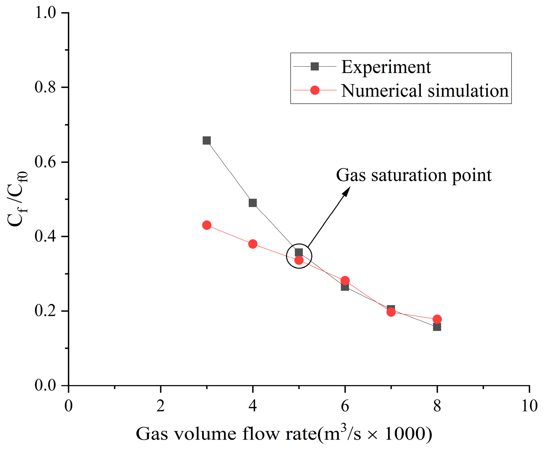
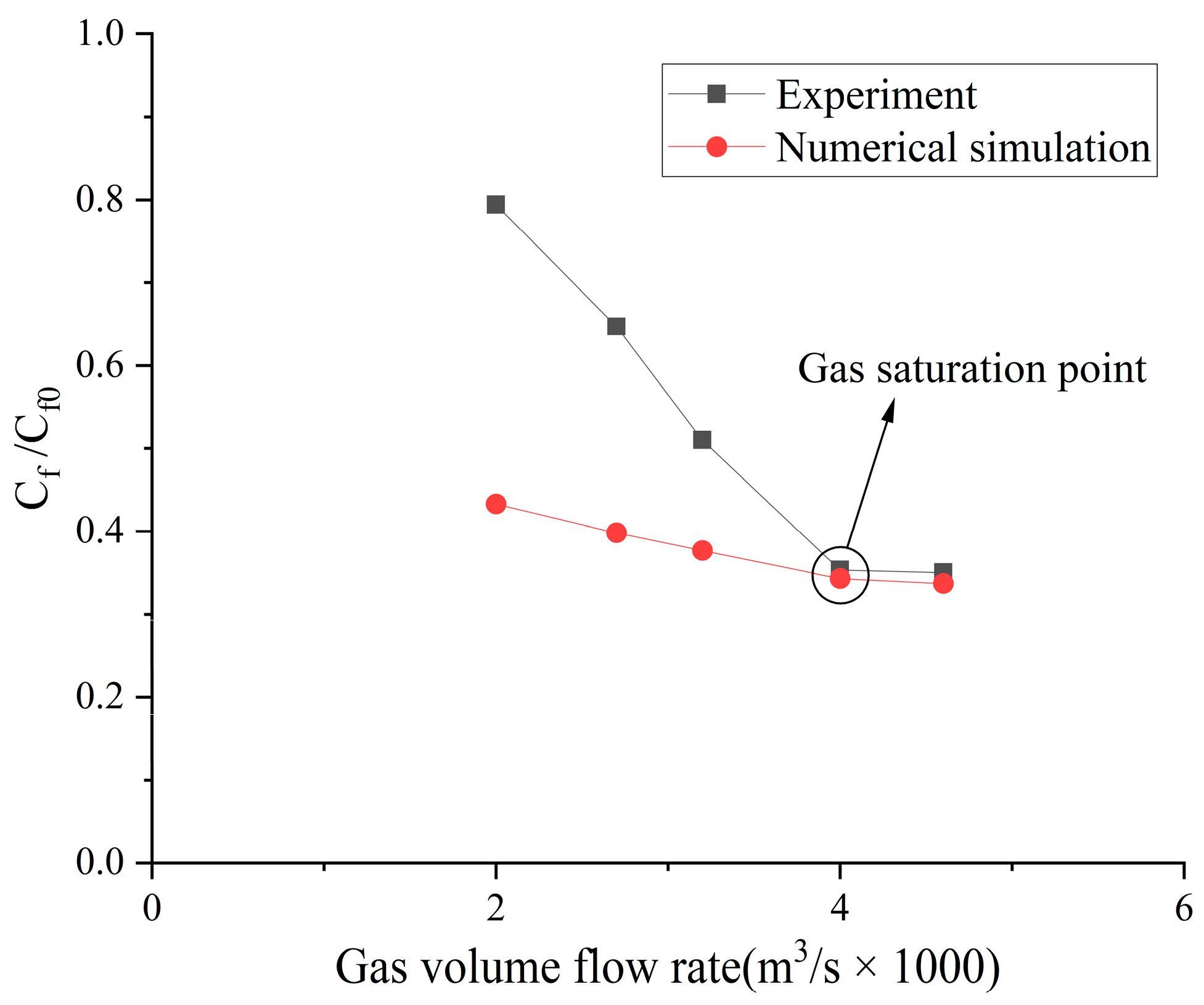
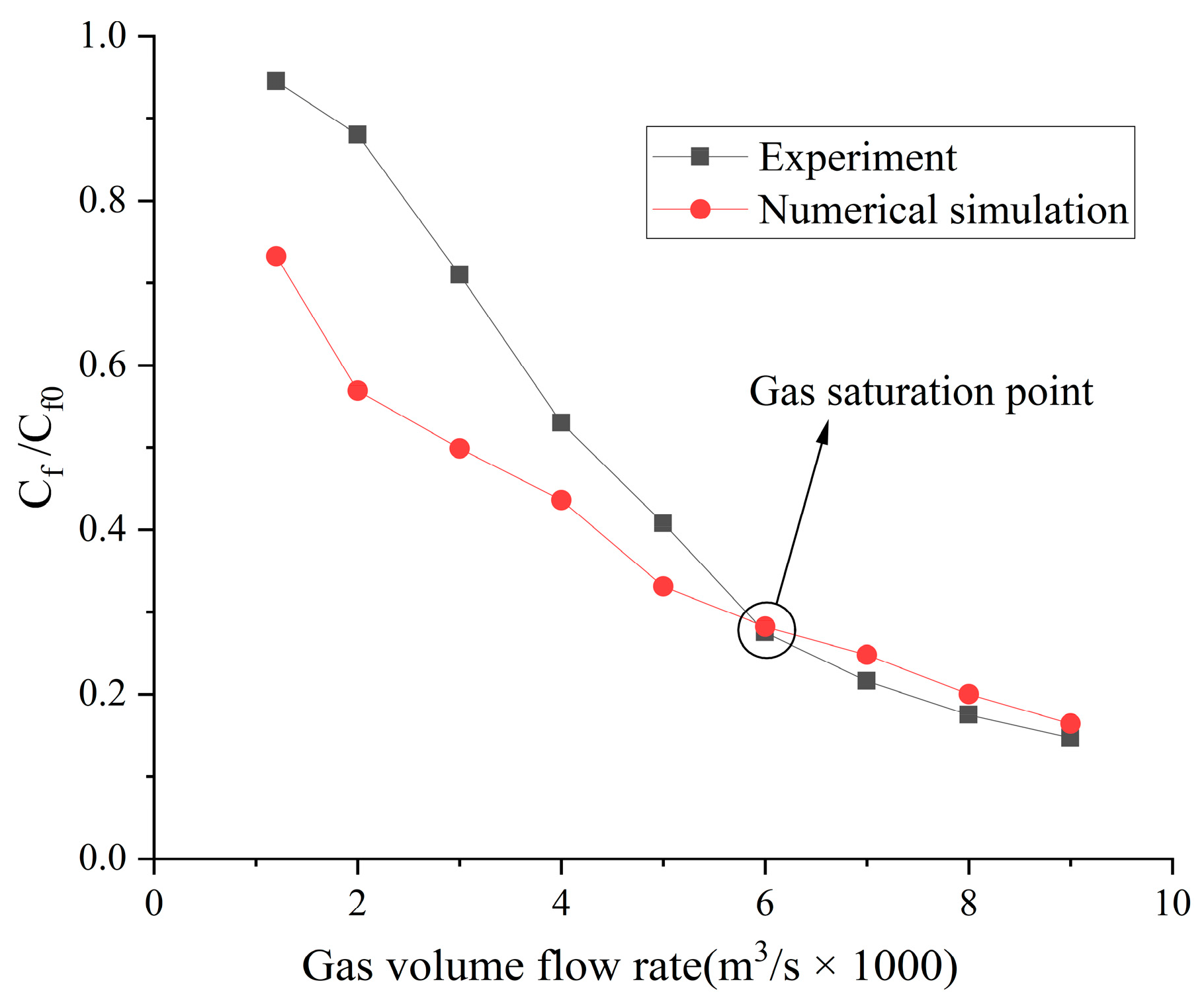
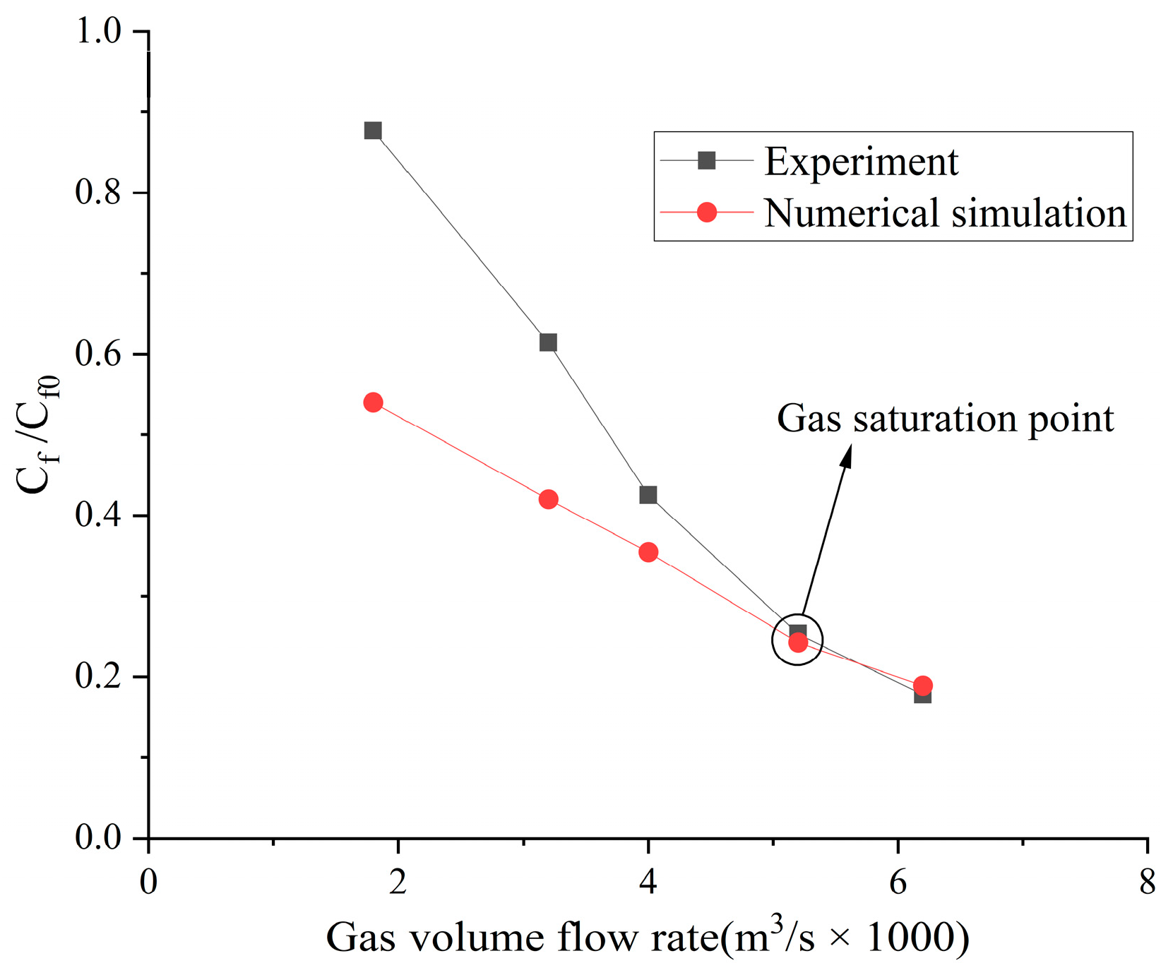
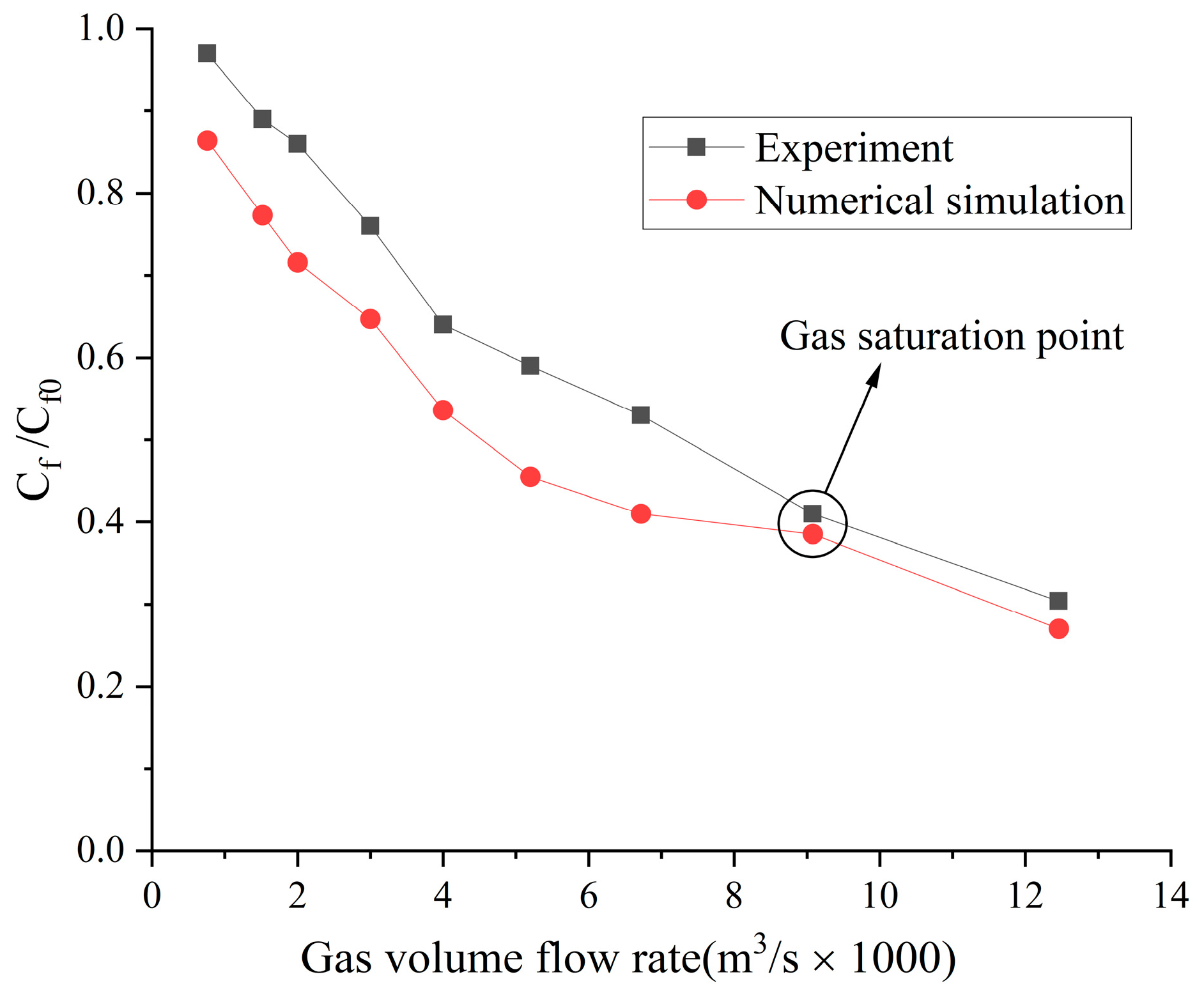
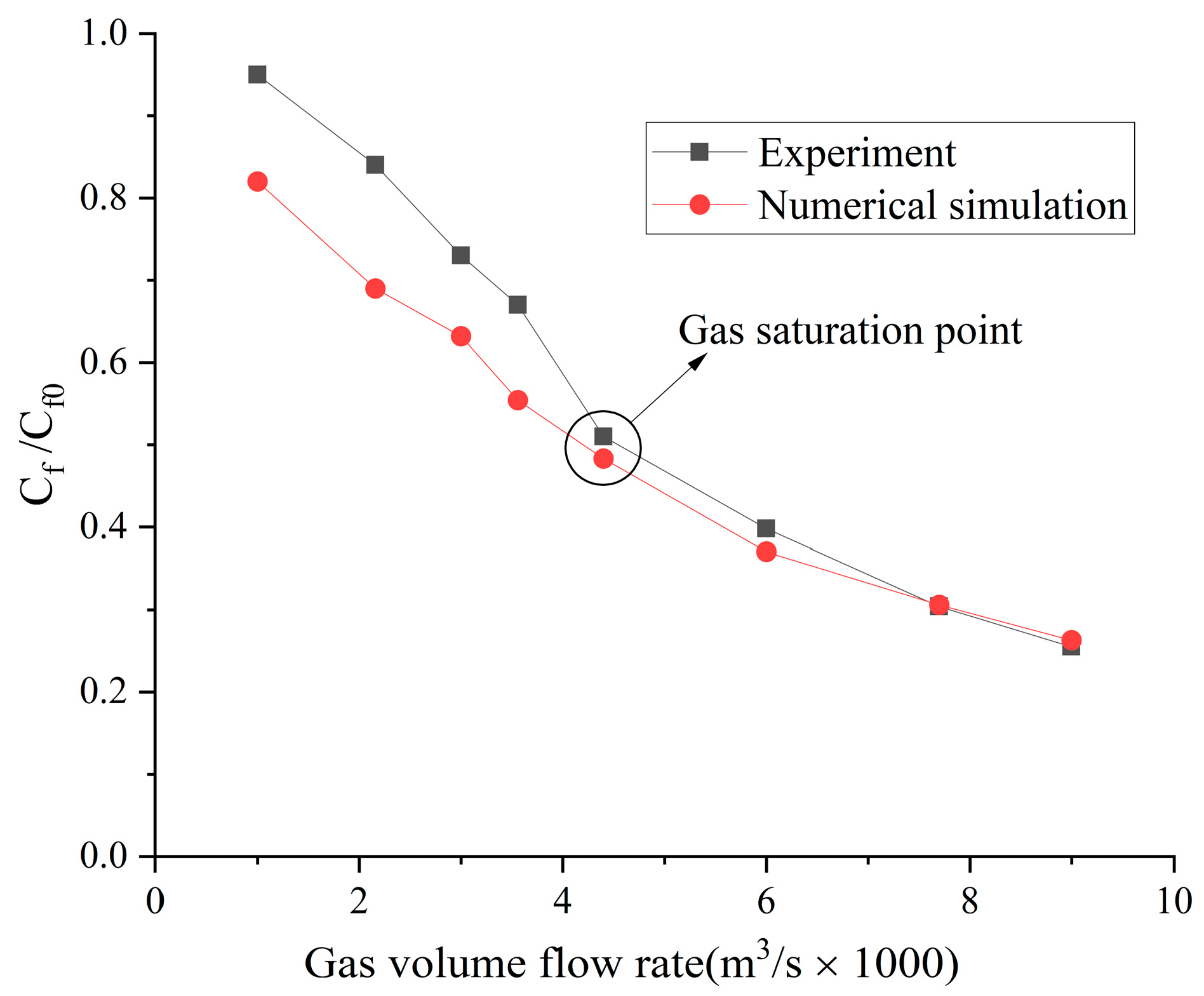
When the volume flow rate of the gas injection is small, the experimental data of the drag reduction ratio is obviously larger than the numerical simulation results, and for different types of gases, their drag reduction ratio decreases at different rates. This is mainly due to the fact that the opening holes ratio in the numerical simulation is larger than that in the experiment. In the case of the same volume flow rate for gas injection, the gas injection speed of simulation is different from that of the experiment due to the difference of the opening holes rate. According to the microbubble drag reduction mechanism, the drag reduction ratio is mainly affected by the diameters of the microbubbles in the boundary layer, which are determined by the gas injection speed [40], and the gas dissolution in the boundary layer further increases this influence. Finally, there is a big gap between the simulation results and the experimental data of the drag reduction ratio;
(2)
With the increase in the volume flow rate of gas injection, when the volume flow rate reaches a certain value, the value of the drag reduction ratio in the experiment is very close to the numerical simulation result, and this close point is marked in the figure, which is defined as the gas saturation point. The existence of the gas saturation point indicates that the gas injection velocity no longer influences the diameters of the microbubbles in the boundary layer. Observing Figure 7, Figure 8, Figure 9 and Figure 10, it can be seen that there are gas saturation points for different types of gases, but these points correspond to different volume flow rates. Observing the volume flow rate of the gas saturation point, it can be seen that helium is about 0.004 m3/s, air and argon are about 0.005 m3/s, argon is slightly larger than air and carbon dioxide is about 0.006 m3/s. The reason why the volume flow rate of these gas saturation points is different is that among these gases, helium has the smallest solubility in water and the smallest influence on the formation of microbubbles in the boundary layer. Therefore, the saturation point of helium corresponds to a smaller gas injection flow rate. Air is more soluble than helium, and argon is slightly more soluble than air. The solubility of carbon dioxide is the largest, which also has the largest influence on the formation of microbubbles in the boundary layer, so the gas saturation point of carbon dioxide corresponds to a larger gas injection flow rate;
(3)
As can be seen from Figure 7, Figure 8, Figure 9 and Figure 10, where the gas saturation point is passed, if the volume flow rate of gas injection continues to increase, the numerical simulation results of the drag reduction ratio of all gases are basically consistent with the experimental data. This is because the gas injection speed and dissolution in the boundary layer no longer affect the diameters of microbubbles in the boundary layer, and the drag reduction ratio completely depends on the volume flow rate of the gas injection. Under the condition that the volume flow rate is the same, the numerical results are basically the same as the experimental data;
(4)
As can be seen from Figure 11, Figure 12 and Figure 13, the comparison between the simulation results and the experimental data of MBDR of different types of gases after the water tunnel pressure increases is consistent with Figure 7, Figure 8, Figure 9 and Figure 10. The volume flow rate of different types of gas injection still has a gas saturation point, but the volume flow rate corresponding to the gas saturation point increases after the water tunnel pressure increases. In addition, by comparing Figure 7 with Figure 11, Figure 8 with Figure 12 and Figure 9 with Figure 13, it can be seen that the solubility of different types of gases in water is also greatly affected by the water tunnel pressure. Carbon dioxide has the largest solubility, so its gas saturation point corresponds to the largest change in volume flow rate, followed by air, with helium being the smallest. The comparison between the simulation results and the experimental data is in accordance with the law of gas solubility variation with water pressure, which proves the correctness of the numerical model.

5. Conclusions

In this study, a numerical method for MBDR considering gas solubility is presented. A UDF is written to define the mass transfer velocity between the gas and liquid phase during microbubble injection of different types of gases, and the numerical models for MBDR of different types of gases are established. According to the experimental conditions, the numerical studies on MBDR of air, carbon dioxide, helium and argon are carried out, and the numerical simulation results and experimental data are compared and analyzed. Finally, the following conclusions are reached:
(1)
Gas solubility cannot be ignored in the process of MBDR. The drag reduction ratio of gas with greater solubility decreases more slowly, and the drag reduction efficiency of gas with smaller solubility is higher;
(2)
When the volume flow rate of injected gas is small, gas dissolution has a great influence on the drag reduction ratio of different types of gases. The larger the solubility of gas, the larger the drag reduction ratio and the lower the drag reduction efficiency. When the volume flow rate of injected gas is large, the influence of gas dissolution on drag reduction ratio of different types of gases is small;
(3)
When the volume flow rate of the injected gas is small, for the same type of gas, if the volume flow rate of the injected gas is the same, but the injection speed is different, the drag reduction ratio is also different, and the greater the solubility of the gas, the greater the difference in the drag reduction ratio.
By comparing the numerical simulation results of the drag reduction ratio with the experimental data, it can be found that the volume flow rate of different types of gases injected has a gas saturation point, which is the dividing point between a small volume flow rate and the large volume flow rate of injected gas. Moreover, due to the difference in gas solubility, the volume flow rate of different types of gases at the gas saturation point is different. The existence of the gas saturation point only reflects the influence of the gas injection speed on the MBDR efficiency, and this point is also the critical point of the transition from MBDR state to the gas-layer drag-reduction state. In addition, in order to improve the calculation accuracy of the proposed model, further research can be carried out from the following aspects: (1) According to the study condition of the microbubble injection flow field, the appropriate turbulence model can be selected. (2) In order to improve the simulation accuracy of the population balance model and the interphase mass transfer coefficient model, the population distribution of the microbubble diameter generated during gas injection should be studied; and (3) the interphase mass transfer rate during microbubble injection is investigated, and the internal relationship between microbubble drag reduction and interphase mass transfer can be analyzed.

Author Contributions

Conceptualization, H.A.; methodology, H.A.; software, P.Y. and H.Z.; validation, P.Y. and H.Z.; formal analysis, X.L.; investigation, H.A. and P.Y.; resources, H.A.; data curation, P.Y. and H.Z.; writing—original draft preparation, H.A., P.Y., H.Z. and X.L.; writing—review and editing, H.A. and P.Y. All authors have read and agreed to the published version of the manuscript.

Funding

This research received no external funding.

Data Availability Statement

Data are contained within the article.

Conflicts of Interest

The authors declare no conflicts of interest.

Nomenclature

a Area of the gas–liquid interface
b ( v , v ) Breakup rate at which the bubbles of volume v break into the bubbles of volume v
c ( v , v ) Coalescence rate of bubbles with volumes v and v
c v i , v j Bubble coalescence rate
C d Drag coefficient
C l Lift coefficient
C vm Virtual mass force coefficient
d p Bubble diameter
D L Liquid phase diffusion coefficient
D q Diffusion coefficient of the qth component in the fluid
E Henry coefficient
F d , q Drag force
F l i f t , q Lift
F v m , q Virtual mass force
F v o l Surface tension
g V Bubble breakage rate
G b Turbulent kinetic energy caused by buoyancy
G k Turbulent kinetic energy caused by mean velocity gradient
J q Diffusion flux of the qth component in the fluid
K L Gas–liquid interface mass transfer coefficient
m ˙ p q Mass transfer from the pth phase to the qth phase
M q Molar mass of the qth phase
n ( v , x , t ) Number density of bubbles
p i * Equilibrium pressure of the solute in the gas phase
P a g v i , v j Probability that a collision will result in a convergence
Re g Bubble Reynolds number
R p q Interaction force between phases
S ( v , x , t ) Source term of the coalescence and breakup of bubble groups
S c Turbulence Schmidt number
S q Mass transfer rate generated by the qth phase from any source
u b ( v , x , t ) Representative bubble velocity
u ¯ i j Collision characteristic velocity of two bubbles with diameters d i and d j and densities n i and n j
v p q Inter-phase velocity
v q Velocity of the qth phase
v S Bubble slip velocity
x i Actual molar fraction of the solute in the liquid phase
x i * Molar fraction of the solute at equilibrium in the liquid phase
Y m Influence of turbulent pulsating flow on the total dissipation rate
Y q Concentration of the qth component in the fluid
α q Gas phase volume fraction of the qth phase
β ( v , v ) Probability density function of the bubble of volume v breaking into the bubble of volume v
γ ( v ) Number of sub-bubbles of volume v
ε Vortex dissipation in liquid phase
κ q Surface curvature
λ q Bulk viscosity of the qth phase
μ Turbulent viscosity
μ L Represents the liquid viscosity
μ q Shear viscosity of the qth phase
μ t Turbulence viscosity coefficient
ρ Average volume density
ρ q Density of the qth phase
σ k Turbulent Prandtl numbers of the turbulent kinetic energy
σ ε Turbulent Prandtl numbers the dissipation rate
σ q p Tension coefficient between the qth phase and the pth phase
τ ¯ ¯ q Stress tensor of the qth phase
ϕ G Gas content
ω v i , v j Collision frequency

References

  1. Pavlov, G.A.; Yun, L.; Bliault, A.; He, S.L. Air Lubricated and Air Cavity Ships: Development, Design, and Application; Springer: New York, NY, USA, 2020; p. 28. [Google Scholar]
  2. Elbing, B.R.; Winkel, E.S.; Lay, K.A.; Ceccio, S.L.; Dowling, D.R.; Perlin, M. Bubble-induced skin-friction drag reduction and the abrupt transition to air-layer drag reduction. J. Fluid Mech. 2008, 612, 201–236. [Google Scholar] [CrossRef]
  3. An, H.; Pan, H.; Yang, P. Research Progress of Air Lubrication Drag Reduction Technology for Ships. Fluids 2022, 7, 319. [Google Scholar] [CrossRef]
  4. McCormick, M.E.; Bhattacharyya, R. Drag Reduction of a Submersible Hull by Electrolysis. Nav. Eng. J. 1973, 85, 11–16. [Google Scholar] [CrossRef]
  5. Pal, S.; Deutsch, S.; Merkle, C.L. A comparison of shear stress fluctuation statistics between microbubble modified and polymer modified turbulent boundary layers. Phys. Fluids A 1989, 1, 1360–1362. [Google Scholar] [CrossRef]
  6. Deutsch, S.; Castano, J. Microbubble skin friction reduction on an axisymmetric body. Phys. Fluids 1986, 29, 3590–3597. [Google Scholar] [CrossRef]
  7. Fontaine, A.A.; Deutsch, S. The influence of the type of gas on the reduction of skin friction drag by microbubble injection. Exp. Fluids 1992, 13, 128–136. [Google Scholar] [CrossRef]
  8. Deutsch, S.; Money, M.; Fontaine, A.; Petrie, H. Microbubble Drag Reduction in Rough Walled Turbulent Boundary Layers. In Proceedings of the ASME FEDSM’03 4th ASME/JSME Joint Fluids Engineering Conference, Honolulu, HI, USA, 6–10 July 2003; pp. 665–673. [Google Scholar]
  9. Zhu, R.; Zhang, H.; Wen, W.; He, X.; Zhao, C.; Liu, Y.; Zhuang, Q.; Liu, Z. Flow-drag reduction performance of a resident electrolytic microbubble array and its mechanisms. Ocean Eng. 2023, 268, 113496. [Google Scholar] [CrossRef]
  10. Skudarnov, P.V.; Lin, C.X. Drag reduction by gas injection into turbulent boundary layer: Density ratio effect. J. Heat Fluid Flow 2006, 27, 436–444. [Google Scholar] [CrossRef]
  11. Mattson, M.; Mahesh, K. Simulation of bubble migration in a turbulent boundary layer. Phys. Fluids 2011, 23, 045107. [Google Scholar] [CrossRef]
  12. Pang, M.J.; Wei, J.J.; Yu, B. Numerical study on modulation of microbubbles on turbulence frictional drag in a horizontal channel. Ocean Eng. 2014, 81, 58–68. [Google Scholar] [CrossRef]
  13. Rawat, S.; Chouippe, A.; Zamansky, R.; Legendre, D.; Climent, E. Drag modulation in turbulent boundary layers subject to different bubble injection strategies. Comput. Fluids 2019, 178, 73–87. [Google Scholar] [CrossRef]
  14. Velasco, L.J.; Venturi, D.N.; Fontes, D.H.; de Souza, F.J. Numerical simulation of drag reduction by microbubbles in a vertical channel. Eur. J. Mech. B-Fluid 2022, 92, 215–225. [Google Scholar] [CrossRef]
  15. Mohanarangam, K.; Cheung, S.C.P.; Tu, J.Y.; Chen, L. Numerical simulation of micro-bubble drag reduction using population balance model. Ocean Eng. 2009, 36, 863–872. [Google Scholar] [CrossRef]
  16. Yan, W. Numerical Simulation of Microbubble Drag Reduction and Mechanism Analysis. Master’s Thesis, Harbin Engineering University, Harbin, China, 2013. (In Chinese). [Google Scholar]
  17. Pang, M.; Zhang, Z. Numerical Investigation on Turbulence Drag Reduction by Small Bubbles in Horizontal Channel with Mixture Model Combined with Population Balance Model. Ocean Eng. 2018, 162, 80–97. [Google Scholar] [CrossRef]
  18. Qin, S.; Chu, N.; Yao, Y.; Liu, J.; Huang, B.; Wu, D. Stream-wise distribution of skin-friction drag reduction on a flat plate with bubble injection. Phys. Fluids 2017, 29, 037103. [Google Scholar] [CrossRef]
  19. Zhang, X.; Wang, J.; Wan, D. Euler–Lagrange study of bubble breakup and coalescence in a turbulent boundary layer for bubble drag reduction. Phys. Fluids 2021, 33, 037105. [Google Scholar] [CrossRef]
  20. Lyu, X.; Tang, H.; Sun, J.; Wu, X.; Chen, X. Simulation of microbubble resistance reduction on a suboff model. Brodogradnja 2014, 65, 23–32. [Google Scholar]
  21. Wang, T.; Sun, T.; Wang, C.; Xu, C.; Wei, Y. Large Eddy Simulation of Microbubble Drag Reduction in Fully Developed Turbulent Boundary Layers. J. Mar. Sci. Eng. 2020, 8, 524. [Google Scholar] [CrossRef]
  22. Zhao, X.-J.; Zong, Z.; Jiang, Y.-C.; Pan, Y. Numerical simulation of micro-bubble drag reduction of an axisymmetric body using OpenFOAM. J. Hydrodyn. 2019, 31, 900–910. [Google Scholar] [CrossRef]
  23. Wang, B. Numerical Simulation and Mechanism Research on Drag Reduction of Ship by Microbubbles. Master’s Thesis, Harbin Engineering University, Harbin, China, 2012. (In Chinese). [Google Scholar]
  24. Shih, T.-H.; Liou, W.W.; Shabbir, A.; Yang, Z.; Zhu, J. A new k-ε eddy viscosity model for high reynolds number turbulent flows. Comput. Fluids 1995, 24, 227–238. [Google Scholar] [CrossRef]
  25. Schiller, L.; Naumann, A. A drag coefficient correlation. Z. Ver. Deutsch. Ing. 1935, 77, 318–320. [Google Scholar]
  26. Drew, D.A.; Lahey, R.T. Application of general constitutive principles to the derivation of multidimensional two-phase flow equations. Int. J. Multiph. Flow 1979, 5, 243–264. [Google Scholar] [CrossRef]
  27. Legendre, D.; Magnaudet, J. The lift force on a spherical bubble in a viscous linear shear flow. J. Fluid Mech. 1998, 368, 81–126. [Google Scholar] [CrossRef]
  28. Magnaudet, J.J. The forces acting on bubbles and rigid particles. In Proceedings of the ASME Fluids Engineering Division Summer Meeting, FEDSM, Vancouver, BC, Canada, 22–26 June 1997; pp. 22–26. [Google Scholar]
  29. Yeoh, G.H.; Tu, J. Computational Techniques for Multi-Phase Flows; Elsevier Butterworth Heinemann; Elsevier Ltd.: London, UK, 2010; pp. 351–456. [Google Scholar]
  30. Luo, H. Coalescence, Breakup and Liquid Circulation in Bubble Column Reactors. Ph.D. Thesis, Norwegian Institute of Technology, Trondheim, Norway, 1993. [Google Scholar]
  31. Laakkonen, M.; Alopaeus, V.; Aittamaa, J. Validation of bubble breakage, coalescence and mass transfer models for gas–liquid dispersion in agitated vessel. Chem. Sci. 2006, 61, 218–228. [Google Scholar] [CrossRef]
  32. Sander, R. Compilation of Henry’s law constants (version 5.0.0) for water as solvent. Atmos. Chem. Phys. 2023, 23, 10901–12440. [Google Scholar] [CrossRef]
  33. Resnick, W.; Gal-Or, B. Gas-liquid dispersions. Adv. Chem. Eng. 1968, 7, 295–395. [Google Scholar]
  34. Higbie, R. The rate of absorption of a pure gas into a still liquid during short periods of exposure. Trans. Am. Inst. Chem. Eng. 1935, 31, 365–389. [Google Scholar]
  35. Danckwerts, P.V. Significance of Liquid-Film Coefficients in Gas Absorption. Ind. Eng. Chem. Res. 1951, 43, 1460–1467. [Google Scholar] [CrossRef]
  36. Balcázar-Arciniega, N.; Antepara, O.; Rigola, J.; Oliva, A. A level-set model for mass transfer in bubbly flows. Int. J. Heat Mass Transf. 2019, 138, 335–356. [Google Scholar] [CrossRef]
  37. Macfarlan, L.H.; Phan, M.T.; Bruce Eldridge, R. A volume-of-fluid methodology for interfacial mass transfer. Chem. Eng. Sci. 2023, 275, 118720. [Google Scholar] [CrossRef]
  38. Li, W.-L.; Wang, J.-H.; Lu, Y.-C.; Shao, L.; Chu, G.-W.; Xiang, Y. CFD analysis of CO2 absorption in a microporous tube-in-tube microchannel reactor with a novel gas-liquid mass transfer model. Int. J. Heat Mass Transf. 2020, 150, 119389. [Google Scholar] [CrossRef]
  39. The Engineering ToolBox. Gases Solved in Water—Diffusion Coefficients. 2008. Available online: https://www.engineeringtoolbox.com/diffusion-coefficients-d_1404.html (accessed on 13 December 2023).
  40. Hashim, A.; Yaakob, O.B.; Koh, K.K.; Ismail, N.; Ahmed, Y.M. Review of micro-bubble ship resistance reduction methods and the mechanisms that affect the skin friction on drag reduction from 1999 to2015. J. Teknol. 2015, 74, 105–114. [Google Scholar]
Figure 1. Schematic diagram of the experimental model.
Inventions 09 00007 g001
Figure 2. Physical model of the vehicle.
Inventions 09 00007 g002
Figure 3. Computing domain and grid division. They can be listed as: (a) Description of the calculation domain of the vehicle; (b) description of grid division of the computational domain.
Inventions 09 00007 g003
Figure 4. Meshing of the vehicle surface in the calculation domain. The arrows represent detail enlargements.
Inventions 09 00007 g004
Figure 5. Drag reduction ratio of different types of gas varies with the volume flow rate of injected gas in the experiment. The experimental data described in the figure comes from the water tunnel experiment [7].
Inventions 09 00007 g005
Figure 6. Drag reduction ratio of different types of gas in the numerical simulation varies with the volume flow rate of injected gas.
Inventions 09 00007 g006
Figure 7. Comparison of numerical results and experimental data of drag reduction ratio during air injection. Tunnel pressure = 15 psi.
Inventions 09 00007 g007
Figure 8. Comparison of numerical results and experimental data of drag reduction ratio during CO2 injection. Tunnel pressure = 15 psi.
Inventions 09 00007 g008
Figure 9. Comparison of numerical results and experimental data of drag reduction ratio during Helium injection. Tunnel pressure = 15 psi.
Inventions 09 00007 g009
Figure 10. Comparison of numerical results and experimental data of drag reduction ratio during Argon injection. Tunnel pressure = 15 psi.
Inventions 09 00007 g010
Figure 11. Comparison of numerical results and experimental data of drag reduction ratio during air injection. Tunnel pressure = 30 psi.
Inventions 09 00007 g011
Figure 12. Comparison of numerical results and experimental data of drag reduction ratio during CO2 injection. Tunnel pressure = 30 psi.
Inventions 09 00007 g012
Figure 13. Comparison of numerical results and experimental data of drag reduction ratio during Helium injection. Tunnel pressure = 30 psi.
Inventions 09 00007 g013
Table 1. Model parameter.
Model Length
L (mm)
Diameter of the Model D (mm)Location of Gas Injection
L1 (mm)
63289146.5
Table 2. Henry coefficients for four gases at 20 °C.
Gases Henry   Coefficient   ( m 3 P a / m o l )
helium2.839 × 105
air1.359 × 105
carbon dioxide3.09 × 102
argon7.14 × 103
Table 3. Diffusivity coefficients of four gases in water.
GasesDiffusivity Coefficient
D L ( m 2 / s )
helium4.8 × 10−9
air3.23 × 10−9
carbon dioxide1.99 × 10−9
argon2.5 × 10−9
Table 4. Parameters for the initial boundary conditions.
ParametersValues
Inlet Velocity13.7 m/s
Temperature20 °C
Density of Water998 kg/m3
Viscosity of Water1.003 × 10−3 kg/m
Inlet Pressure (Gauge)0 Pa
Outlet Pressure (Gauge)0 Pa
Tunnel Pressure15 psi, 30 psi
Table 5. Grid independence analysis.
Mesh GenerationGrid Size (mm)Number of Grids (million)Time Step (ms)CourantDrag Reduction Rate (%)
Fine grid0.83.50.06183.73
Medium Grid1.31.80.10184.61
Coarse grid2.11.20.16186.87
Table 6. Parameters of working condition 1.
GasesTunnel Pressure (psi)Free-Stream Speed (m/s)Gas Volume Flow Rate (m3/s × 103)
air1513.71, 2, 3, 4, 5, 6, 7, 8.
carbon dioxide1513.71.2, 2, 3, 4, 5, 6, 7, 8, 9.
helium1513.71, 2, 2.7, 3.2, 4, 4.6.
argon1513.71.8, 3.2, 4, 5.2, 6.2.
Table 7. Parameters of working condition 2.
GasesTunnel Pressure (psi)Free-Stream Speed (m/s)Gas Volume Flow Rate (m3/s × 103)
air3013.70.73, 1.5, 2, 3, 4, 5.2, 6.7, 8, 9.1, 12.5.
carbon dioxide3013.70.88, 2, 3, 3.9, 4.9, 6.5, 8.4, 9.6, 12.
helium3013.71, 2.2, 3, 3.6, 4.4, 6, 7.7, 9.
Disclaimer/Publisher’s Note: The statements, opinions and data contained in all publications are solely those of the individual author(s) and contributor(s) and not of MDPI and/or the editor(s). MDPI and/or the editor(s) disclaim responsibility for any injury to people or property resulting from any ideas, methods, instructions or products referred to in the content.

