Computer Vision Algorithm for Characterization of a Turbulent Gas–Liquid Jet

Abstract

A computer vision algorithm to determine the parameters of a two-phase turbulent jet of a water-gas mixture traveling at a velocity in the range of 5–10 m/s was developed in order to evaluate the hydrodynamic efficiency of mass exchange apparatuses in real time, as well as to predict the gas exchange rate. The algorithm is based on threshold segmentation, the active contours method, the regression of principal components method, and the comparison of feature overlays, which allows the stable determination of jet boundaries and is a more efficient method when working with low-quality data than traditional implementations of the Canny method. Based on high-speed video recordings of jets, the proposed algorithm allows the calculation of key characteristics of jets: the velocity, angle of incidence, structural density, etc. Both the algorithm’s description and a test application based on video recordings of a real jet created on an experimental prototype of a jet bioreactor are discussed. The results are compared with computational fluid dynamics modeling and theoretical predictions, and good agreement is demonstrated. The presented algorithm itself represents the basis for a real-time control system for aerator operation in jet bioreactors, as well as being used in laboratory jet stream installations for the accumulation of big data on the structure and dynamic properties of jets.

1. Introduction

Intense fluid jetting is a key technical element in a number of industrial devices, e.g., grinding [1,2,3], cutting [4,5], etc. The detailed characterization of multiphase gas–liquid flows is critical in metallurgical processes, the design of efficient air and ground devices, combustion devices in aircraft and aerospace systems, and engines in transportation and marine engines, as well as when developing new technologies leading to technological advances [6,7,8,9]. The system’s jet parameters determine the characteristics of the device and its efficiency and also provide relevant information for industrial biotechnology due to the increased demand for efficient technological solutions in the field. Devices and apparatuses are important components when jets play the role of a kinetic mixer [10,11], providing intensive mass exchange in the volume of the liquid.

Jet stream bioreactors [12,13] represent a type of machine with the recirculation of the liquid and gas phases caused by generated multiscale gas–liquid jets with a high volume content of gas bubbles. The behavior of the jet can be characterized as a high-turbulence physical process, frequently leading to technical problems related to flow control, analyzing its parameters, and further optimizing design elements such as the nozzle and jet pump. There is a liquid core region, the structure of which is affected by interaction with the gas phase, which leads to its significant change, i.e., deformation of the continuous flow.

The interaction of the liquid and gas phases generates a number of physical phenomena, such as the exchange of momentum and energy between the flow phases, a unique structure of flow pulsations, phase transitions, bubble effects, and dissolution processes in the gas phase, which significantly change the characteristics of the heat and mass transfer [14,15,16]. External forces acting on the jet surface can lead to oscillations and perturbations of the jet boundaries. This oscillation can intensify and eventually lead to the disintegration of the flow into small droplets, or even the flow’s complete destruction.

The peculiarity of these devices is that they can combine high jet flow energies and considerable apparatus sizes. The kinetic energy of a jet represents the main source of turbulence and drives the microscale mixing of the liquid and gas phases by turbulent diffusion. This means that high specific costs are associated with the formation of the jet stream. In the case of such a jet having low efficiency, i.e., its significant destruction, the costs become significant.

Therefore, a fundamental physical understanding of jet formation and behavior is an important research and operational challenge.

A number of techniques are known to be applicable to the study of gas–liquid jets due to their wide application in technical and biotechnical problems [17]. Recently, various studies have relied on the computational fluid dynamics (CFD) modeling of hydrodynamic processes in bioreactors [13,18,19,20,21,22,23,24]. The mathematical description of multiphase flows is complicated in many aspects due to the peculiarities associated with the mutual influence of continuous and dispersed phases. Therefore, the bubble flow [13,25,26,27], annular flow [28], and more complex flows [21,23,29] have received a new wave of study. Important mass transfer characteristics of the process are studied in [12,19,23,30]. In addition to characterizing multiphase flows, CFD methods have found application in solving the problem of achieving optimal performance in bioreactors [22]. However, the problem is always associated with the description of multiphase multicomponent flows with developed turbulence, which makes the task of computer simulation computationally complex. Meanwhile, the list of factors affecting the formation of jets is quite significant, and experimental studies and objective monitoring remain valid sources of data on jets’ properties.

It has now been shown that, in a number of areas, new deep and machine learning methods, particularly computer vision (CV) methods, outperform previous, state-of-the-art methods [31,32,33]. These papers often represent general information on new methods or compare them. With recent advances in digitization and big data analytics, digital tools are gradually beginning to be adopted in biotechnology research. Biological, hydrodynamic, and heat and mass transfer processes in bioreactor (fermenter) circuits are key targets for such digital approaches, as these processes are often complicated to analyze [34,35,36,37]. The maximum bioreactor efficiency is primarily determined by gas phase transfer through the gas–liquid interface. Therefore, hydrodynamic parameters such as the bubble sizes in the gas–liquid stream significantly influence the flow behavior and determine the overall performance of the fermenter. Machine learning algorithms show advantages in terms of accuracy with respect to bubble sizing [38,39,40]. Used to capture real-time parameters and support decision making to control and optimize key performance and safety indicators of the biosynthesis process, success stories are increasingly appearing in the scientific and technical literature and reports, where computer vision is proving to be not only one of the most efficient but also one of the most affordable non-destructive methods compared to expensive, invasive methods that require additional, sometimes redundant, equipment with sets of sensors, transducers, detectors, and neural networks, which, in turn, are also attractive tools for a number of their characteristics, such as accuracy and the ability to handle small objects.

Experiments show that the best mixing in jet bioreactors is provided by a coherent jet with the lowest mass loss in the form of detached droplets and the highest vertical velocity. Visually, such a jet is characterized by the smallest opening angle and the absence of edge fluctuations. However, unlike other technical devices, in jet bioreactors, the water jet at the nozzle outlet contains a large amount of gas phase (up to a volume proportion of 1:1 [41]). Depending on the liquid delivery mode determined by the pump operation, such a flow can be a bubble flow, an annular flow, or a set of many individual jets and droplets. Thus, the CV observation of the shape, structure, and velocity of the jet becomes one of the ways to select the optimal mode of operation of the bioreactor.

The following sections will propose a computer vision algorithm that allows the stable processing of a gas–liquid video obtained from a high-speed camera.

2. Materials and Methods

Various parameters, such as the jet opening angle, contour deviations, and jet velocity, are known to have a significant impact on the breakup length and pattern of liquid jets [42] (see Figure 1).

The angle and deviations from the line of a liquid jet’s contour determine its shape. A jet with a narrow angle and few deviations will have a more streamlined shape, resulting in a longer breakup length. On the other hand, a wider angle and more deviations in the contour can lead to an irregular shape, causing the jet to break up sooner.

The velocity of the liquid jet plays a crucial role in its breakup length and pattern. Higher velocities tend to create thinner, more elongated jets that experience greater aerodynamic instability. This instability might cause the jet to break up earlier and result in a more chaotic breakup pattern. Conversely, lower velocities lead to thicker jets that are relatively more stable and have a longer breakup length. However, as the jet speed increases, both an increase and a decrease in breakup length can occur, depending on the speed range in which the experiments are carried out. In the case of a low speed of turbulent flow, an increase will be observed, and when a certain critical point is reached, the increase will be replaced by a decrease. The conditions at the jet boundary, such as the presence of surrounding gas or a solid surface, can significantly influence the breakup of the liquid jet. For instance, if the jet is fully surrounded by a gas medium, it experiences less resistance and can travel for a longer distance before breaking up. Alternatively, if the jet comes into contact with a solid surface, it may undergo secondary breakup or atomization, leading to a shorter breakup length and a more dispersed pattern.

2.1. Data Parameters and a General Description of the Order of Operations for Algorithms

In order to evaluate the characteristics of the jet and subsequently relate them to the parameters of the apparatus for its production, we have developed algorithms based on computer vision methods. High-speed camera records provide initial data.

Each video after loading is converted into a three-dimensional array of scalars and pixel intensities. Here, indices along one of the axes allow us to work with individual frames. We use the grayscale color model so that the algorithms that we implement do not depend on the color features of the lighting equipment or the environment. It also allows a reduction in the weight of the data in the array itself, which is very important for the fast execution of algorithms. Next, we normalize the data so that, regardless of the format of the source data, the minimum intensity is 0 and the maximum is 255. After this, to determine the parameters of a gas–liquid jet, we propose the following set of steps:

1.

detection of the edge of the jet (gas–liquid boundary) in the form of a set of coordinates of points on this boundary for each frame of the video sequence;

2.

determination of the straight line of the best approximation to points on the jet boundary;

3.

calculation of the root-mean-square deviation of points on the jet boundary from the straight line of best approximation;

4.

calculation of the angle of deviation of the line of the best approximation from the vertical for both the right and left edge of the jet; the difference between these angles is equal to the angular expansion of the jet.

Using computer vision algorithms, it is necessary to take into account the features of specific data sets. In our case, there is heterogeneity in the images, i.e., areas of high and low pixel intensity. The image regions between these irregularities can be used to detect jet boundaries. However, the original image does not have high contrast, and it also contains noise, i.e., the visible boundaries are blurred. This is due to the fact that the flows and environments studied impose physical limitations on the image quality. The selected computer vision methods should be sufficiently resistant to noise and blurring.

The study of the data by plotting pixel intensity distributions (Figure 2) is an important step in choosing the parameters of filters for image processing, as well as the parameters of methods for the detection of jet boundaries.

However, the mere presence of heterogeneity is not enough. Of great importance is the relative position of such pixels. In this vein, it is necessary to take into account the characteristic pixel intensity gradients that the images have, since it is the magnitude of this gradient that makes it possible to clearly detect the border. Accordingly, the algorithm used for border detection must be able to work with exactly the range of gradients that we observe. In our case, the boundaries are very blurred; the gradients are small, and, accordingly, purely gradient methods are less preferred. Another limitation is the physical continuity of the boundary of the gas–liquid jet. The algorithm must be able to construct a continuous boundary, even if the jet boundaries appear steep in the image.

Another feature of our data is the dynamic changes over time (Figure 3). The average brightness intensity of the pixels and their distribution in the frame can vary very significantly as we move from frame to frame. Accordingly, methods applied to such data must be robust to such dynamic changes.

The dynamic nature of the data variability (Figure 3) corresponds to the physical causes and hydrodynamic features of the studied gas–liquid system. This must also be taken into account since such variability is also observed in the form of boundary deviations. As the jet stream angle increases, the size of the area corresponding to the jet will increase, which means that the average pixel intensity in the frames will also change.

2.2. Active Contours Method for Jet Edge Detection

A number of publications describe several approaches to determining the jet edge, i.e., the gas–liquid interface [43,44,45,46]. All methods are based on gradient methods, primarily on the Canny edge method [47]. However, to find the edges of the jet on our data, these methods produce a lot of side contours. Therefore, it was decided to use the active contour model (ACM) method [48,49] to determine the boundaries of objects on 2D images. In ACM, the object boundary is considered as an elastic line (spline) specified by the coordinates (x, y) of the points on it, and the functional $\mathrm{E}$ is minimized [50]:

$$\mathrm{E}=\underset{0}{\overset{1}{\int }}\left[{\mathrm{E}}_{\mathrm{int}}\left(\mathrm{v}\left(\mathrm{s}\right)\right)+{\mathrm{E}}_{\mathrm{image}}\left(\mathrm{v}\left(\mathrm{s}\right)\right)\right]\mathrm{ds}$$

(1)

where $\mathrm{v}\left(\mathrm{s}\right)=\left(\mathrm{x}\right(\mathrm{s}),\mathrm{y}(\mathrm{s}\left)\right)$ is the parametric representation of the contour, and $s\in [0;1]$ is the contour parameter.

${\mathrm{E}}_{\mathrm{int}}\left(\mathrm{v}\left(\mathrm{s}\right)\right)=\alpha {\left|{\mathrm{v}}_{\mathrm{s}}\right|}^2+\beta {\left|{\mathrm{v}}_{\mathrm{s}\mathrm{s}}\right|}^2$ is the internal energy of the spline; ${\mathrm{v}}_{\mathrm{s}}$ and ${\mathrm{v}}_{\mathrm{ss}}$ are the first derivative and the second derivative of $\mathrm{v}$ with respect to s, respectively.

${\mathrm{E}}_{\mathrm{image}}=-\gamma {|\nabla \mathrm{I}(\mathrm{x},\mathrm{y})|}^2$ is the so-called image energy; $\alpha ,\beta$, and $\gamma$ are the parameters of the ACM method. Thus, by minimizing the functional $\mathrm{E}$, it is possible to “pull” the contour to the boundaries with a sharp difference in brightness while, at the same time, avoiding excessively long and crimped contours. If there is a noticeable level of noise and interfering artifacts (for example, splashes) in the image, Gaussian smoothing is first applied to the intensity function $\mathrm{I}(\mathrm{x},\mathrm{y})$ before calculating ${\mathrm{E}}_{\mathrm{image}}$. On the first frame of the video sequence, the points of the beginning and end of the lines of the initial approximation of the jet boundaries are placed, which are then used as initial conditions on all analyzed frames. Moreover, the distance between the upper points of the initial approximation lines is used to obtain the length scale factor (the diameter of the pipe outlet nozzle is known).

Figure 4 shows an example of the application of the ACM method to determine the boundaries of the jet.

Before the analysis of data, it is necessary to align (rotate) the image so that the normal to the plane of the nozzle runs strictly vertically. For a quantitative assessment of such jet parameters as the angle of divergence and fluctuations in the boundary contour, a straight line of best approximation is determined for both edges of the jet. Since the position of the jet in the initial data is close to vertical, the best results for determining the approximating straight line are given by the principal component method (PCA) [50] compared to the least squares method. In the approach that we used, an approximating line was obtained in the form of a sequence of coordinates of its points $\left({\mathrm{x}}_{\mathrm{i}},{\mathrm{y}}_{\mathrm{i}}\right),\mathrm{i}=1\cdots \mathrm{n}$, where the number of points n was equal to their number on the original contour.

The angle of deviation of the line of best approximation of the edge of the jet from the vertical position ${\alpha }_{\mathrm{edge}}$ was calculated as

$${\alpha }_{\mathrm{edge}}={tan}^{-1}\left(\frac{{\mathrm{x}}_{\mathrm{n}}-{\mathrm{x}}_1}{{\mathrm{y}}_{\mathrm{n}}-{\mathrm{y}}_1}\right)$$

(2)

${\mathrm{x}}_1,{\mathrm{x}}_{\mathrm{m}},{\mathrm{y}}_1,{\mathrm{y}}_{\mathrm{n}}$ are, respectively, the $\mathrm{x}$ and $\mathrm{y}$ coordinates of the first and last points on the line of best approximation of the given edge of the jet (see Figure 4).

The difference between the angles ${\alpha }_{\mathrm{edge}}$ of both the right and left edges of the jet is equal to the angular opening (expansion) of the jet. Further, in this article, this value is called the jet angle.

Next, the root-mean-square deviation of the contour points of the jet edges from the corresponding approximating straight lines is calculated. This parameter characterizes numerically the oscillatory behavior of the jet edges (boundaries).

2.3. Method for Determination of the Flow Velocity in a Jet

An important characteristic of the processes occurring in the bioreactor is the rate of liquid supply to it. Measuring the solution pumping rate with a flow meter is not always possible. Therefore, we have developed an approach to estimate the linear jet flow velocity using computer vision methods. When analyzing the original video recordings, it can be seen that there are structures on the surface of the jet that move, as we assume, at the speed of the jet itself. The “lifetime” of such structures is mainly from 2 to 5 frames of video recording produced at a speed of 1000 frames per second. It is possible to trace the interframe movement of such structures throughout their existence interval and estimate the average displacement during the interframe interval.

Figure 5c in a later section shows an example of two adjacent frames with an estimated offset of a given structure. The flow velocity estimate is calculated according to

$${\mathrm{v}}_{\mathrm{flow}}=\frac{\mathrm{dy}}{\mathrm{dt}},$$

(3)

where $\mathrm{dy}$ is the interframe shift of the selected structure, $\mathrm{dt}$ is the time interval between adjacent video frames. This approach will give a suitable estimate of the flow velocity only at high shooting speeds, since the lifetime of isolated structures on the flow surface is, according to our estimates, no more than 5–8 $\mathrm{ms}$ (5–8 frames at a shooting rate of 1000 frames per second).

To improve the accuracy of stream velocity estimation, we propose, firstly, to place at least 10 points on each frame—the centers of the structures, the interframe shift of which will be measured. Secondly, such measurements are made on a relatively large number of frames. The obtained values of the flow rate estimates are subjected to statistical processing. The mean value $\mathrm{v}$ and the root-mean-square spread ${\sigma }_{\mathrm{x}}$ are calculated. Values that do not fall within the interval $\mathrm{v}\pm 2{\sigma }_{\mathrm{v}}$ are excluded from further analysis. The average value of the remaining values is the estimate of the flow velocity.

To automatically select the centers of the structures whose interframe shift will be evaluated, the following approach is proposed. Preliminarily, Gaussian smoothing of the processed frame of the video sequence is performed in order to reduce the influence of random fluctuations. Next, the image is binarized with a threshold, which is currently set manually. It is necessary to adjust the threshold so that only a few (about 10) individual small areas remain. All the indicated transformations of the image are performed only between the boundaries of the flow found earlier. Figure 6 shows an example of the original frame and that after binarization. To reduce the size of the areas that will be followed further, the erosion procedure was applied to them [47].

The centers of the found areas are taken as the centers of the structures, the interframe shift of which will be measured to estimate the flow rate. To find the coordinates of the selected structure on the next frame, the method of maximum mutual spatial correlation is used [51,52].

We carried out a visual comparison of the results of manual marking with the results of the algorithm (Figure 7). The resulting differences are practically insoluble visually. Calculating the errors for such algorithms is quite complicated since the boundaries of the jet are not known in advance and the data are obtained experimentally. However, by performing a similar assessment for a synthetic image of a jet, we can estimate the root-mean-square error as 0.07 pixels.

The algorithm was also compared with a well-known method of determining edges in images, i.e., the Canny edge method [47]. Figure 8 shows an example of the application of the Canny method to a jet image, both synthetic and experimentally obtained. On the synthetic image, the Canny method showed a good result, in contrast to the image obtained experimentally. It can be seen that due to the presence in the real image of a large number of objects and structures with complex boundaries, the Canny edge method, on the one hand, allowed many false detections of edges; on the other hand, there are discontinuities at the detected liquid–gas interface. Finally, it can be concluded that, with no special preprocessing, the algorithms based on the Canny method with respect to image series are unstable.

Thus, the proposed algorithm for the detection of the liquid–gas interface on experimentally obtained images, being almost completely automatic, is practically not inferior in accuracy to manual tracing.

2.4. Jet Properties at Different Flows: Algorithm Usage

The developed algorithms were tested on the example of data obtained with the experimental setup, which is represented by a jet-stream-type mass exchange apparatus; see Figure 9. Previously, such a setup was used in the study of bubble generation by computer vision methods [38].

The mass exchange apparatus in Figure 9 is a closed hydrodynamic circuit. The mixing and circulation of the liquid are carried out using the circulation pump. Along the flow of the liquid, the pipeline and heat exchanger are located. The aerator mixes the sucked gas and liquid phases and then accelerates the gas–liquid jet and penetrates into the liquid inside the machine body, where the video is taken through the viewing window.

The operating mode of this setup is regulated by the rotation speed of the pump, which in turn depends on the value of the frequency converter. The pump creates a flow of liquid, which is saturated with gas by passing through the aerator and descends through the pipe into the tank, forming a high-turbulence gas–liquid jet. Due to the complex flow kinetics, the characteristics of the jet will be determined by many factors, such as the nozzle shape, gas phase fraction, medium structure, pressure, turbulent energy, etc.

Thus, it is difficult to consider all the physical factors and predict the jet characteristics that affect the convection and, ultimately, mass transfer in the setup machine body (the tank). One solution is to create advanced CFD models, but this method is computationally intensive and needs experimental verification. Therefore, we investigated the task of processing a set of experimental video recordings of a jet flow in the setup at different pump operation modes. Note that the video records were made in a foggy environment inside the tank, caused by the peculiarities of the fluid dynamic currents inside the apparatus. Thus, such data are a good test for the proposed computer vision algorithms.

Table 1. The description of the observed jet structures on the video data for different setup regimes. By the regime, we consider the value on the frequency converter that controls the pump performance.

Setup Regime, Hz	Jet Structure	Comment
20	Split	The water flow is insufficient to fill the entire nozzle volume. The jet is discontinuous and represented by split streams.
25	Split	Similar to the regime of 20 Hz.
30	Ring (annular)	The fluid flow is uninterrupted along the nozzle walls, but there is not enough fluid to fill the entire nozzle cross-section. A ring current is observed.
35	Uniform	The liquid flow fills the nozzle completely, and the jet appears to be continuous, in which the liquid and gas fractions are uniformly distributed.
40	Uniform	Similar to the regime of 35 Hz.
45	Uniform	Similar to the regime of 35 Hz.
50	Uniform	Similar to the regime of 35 Hz.

shows the investigated operating modes of the unit and the visually observed structural features of the jet.

Figure 10 shows three types of gas–liquid jet flow structures. The images are presented without processing; the blurring is due to the highly foggy environment inside the tank. All structures are united by the presence of sharp jet boundaries, which form the divergence of the jet. By total jet divergence, we refer to an angle 2$\alpha$ where a is calculated for each edge of the jet, as shown in Figure 4.

Figure 5 shows the steps of applying the algorithm to calculate the characteristic velocity of a gas–liquid jet. Figure 5a schematically represents the necessary labels that will be used in constructing the contours in the active contours method. Figure 5b shows the continuous curves for one gas–liquid jet flow structure, which characterizes the contours from which the jet angle will be calculated. Figure 5c shows schematically the velocity calculation for two consecutive frames using the threshold segmentation method. The threshold segmentation method identifies specific areas corresponding to highlights in two adjacent frames. Next, the vertical shift in pixels is calculated for each selected segment. Then, the displacement value is converted into a physical distance by scaling at the extreme points of the pipe (fixed diameter). In order to calculate the segment speeds, the resulting distance in millimeters is divided by the time between two successive frames. Averaging the obtained velocities makes it possible to calculate the characteristic velocity of the gas–liquid jet under the assumption that the velocity of the glare along the vertical axis is approximately equal to the velocity of the flow.

All videos discussed in this paper were captured by a Sony ZV-1 (Sony Corp., Beijing, China) high-speed (1000 frames per second) video recorder. The deviation of the jet contours illustrates the pulsation of internal flows and their properties. For the best possible convection of the medium in the tank, the jet must be continuous, forming a single mass body, and have downward directed velocities at all points in the volume. This means that the effective jet must have the lowest edge deviation. At the same time, to increase convection, the jet must have the maximum momentum, which refers to the largest vertical velocity component. For the 20–50 Hz regimes (see Table 1) of the investigated jet stream setup, the liquid and gas phase fluxes were measured in experiments earlier. The measured curves are presented in Figure 11.

The volumetric fluid flow rate was measured as a function of the pump capacity and is a smooth curve. The gas volume flow rate provided by the free suction of the aerator was measured by anemometry and represents a significantly non-linear curve. An important characteristic of the aerator is the ejection coefficient, which is the ratio of the volumetric gas flow rate to the liquid flow rate. In Figure 11, one can see that the ejection coefficient of the aerator of the experimental setup varies non-monotonically, which indicates a change in the gas content and in the structure of the gas–liquid flow in the jet. Thus, the jet characteristics are difficult to predict due to the complex nonlinear relationship between the ejection process and pump performance and cannot be reliably interpolated or extrapolated.

3. Results and Discussion

In this section, we analyze the results of applying the presented algorithm to the jet videos obtained using the experimental setup considering different modes of pump operation (which is equivalent to changing the input mechanical energy, since all the energy in the setup is inputted only by the rotating pump blades). For simplicity, we will denote the pump modes by the frequency of the electric current due to its linearly related quantities.

For each mode of the setup (20 Hz, 25 Hz, 30 Hz, 35 Hz, 40 Hz, 45 Hz, 50 Hz), frame-by-frame measurements of the jet angle, edge divergence, and flow rate parameters were performed. For this purpose, video recordings with a length of 1000 frames (1 s of physical time) were selected. Figure 12, Figure 13, Figure 14 and Figure 15 represent the results of these studies. Table 1 summarizes the qualitative characteristics of the jet structure observed visually.

Note that in the 20 Hz mode, the jet with a discontinuous split flow structure (Figure 10a) has a large angle (up to 23 degrees) and average deviation (about 9 mm). From the physical point of view, this is explained by the low energy and flow density (because the pump fluid supply is minimal compared to other modes), as well as the fact that the fluid is not sufficient, not only to fill the entire nozzle but also to form a film flow. As a result, individual jets fly out of the nozzle and then disintegrate into droplets and fly in different directions. Such a jet does not provide the penetration of the water column in the bioreactor tank, which means that mixing and mass transfer are at a very low level.

In the 30 Hz mode, a jet with continuous boundaries is formed at the nozzle outlet. Visually, it can be seen that the boundaries of the jet are quite thin, and, in the center of the flow, there is a solid gas phase. This type of flow is usually called a ring flow. In this case, the angle is decreased by almost five times compared to the 20 Hz mode, to about 5 degrees, while the mean edges’ deviation is decreased by about two times to 4–5 mm. These observations are attributed to an increase in the fluid flow, which is sufficient to form a continuous ring. The fluid ceases to disintegrate into droplets and is no longer dispersed, as was observed in the case of the 20 Hz mode.

The bulk of the gas moves in the center of the jet separately from the liquid boundary layer, in the structure of which there are few bubbles, and therefore the structure is almost homogeneous. This reduces the deviation of the jet boundaries. In terms of efficiency, such a jet has a good penetration capacity at relatively low pump speeds, but the low gas content makes the jet inefficient in terms of mass transfer: gas does not enter the unit tank in bubble form, and the contact area of the liquid and gas phases as a result is low.

In the 40 Hz setup mode, a continuous gas–liquid jet is observed. The pulsations of the bubble phase cause local turbulence and oscillations of the jet, which can be seen by the increase in the boundary deviation up to 15 mm. At the same time, the jet has a small angle (about 5 degrees), which means that the velocities in the flow have a predominantly vertical direction. Such a jet has a large penetration force while providing not only mixing but also high mass transfer rates.

Increasing the pump rpm after the 40 Hz mode led to the formation of a column of bubbly medium above the nozzle (see Figure 15). Thus, a pressure gradient was formed at the nozzle outlet: the compressed mixture of gas and liquid flies out of the nozzle and sharply decompresses, which leads to an increase in the jet angle up to 12 degrees and the growth of the boundary deviation up to 15 mm. Such a jet has a high momentum and penetration force, but, because of the large angle, the vertical velocity component may be equivalent to a jet in the 40 Hz mode, which would reduce the specific mixing efficiency per unit of energy expended.

In Figure 16, the average angle and edge deviation for different setup regimes are presented. Note the tendency of a decreasing angle and deviation when passing from low-intensity and fluid flow modes, for which split jet flows are observed, to modes corresponding to continuous flows (from 30 Hz). Further, there is a build-up of gas content in the liquid flow, which leads to pulsations and a growth in deviation. When a certain critical mode is reached (in our case, it is 40 Hz), a significant pressure gradient appears at the nozzle outlet, as a result of which the jet is decompressed and its angle increases rapidly along with the deviation.

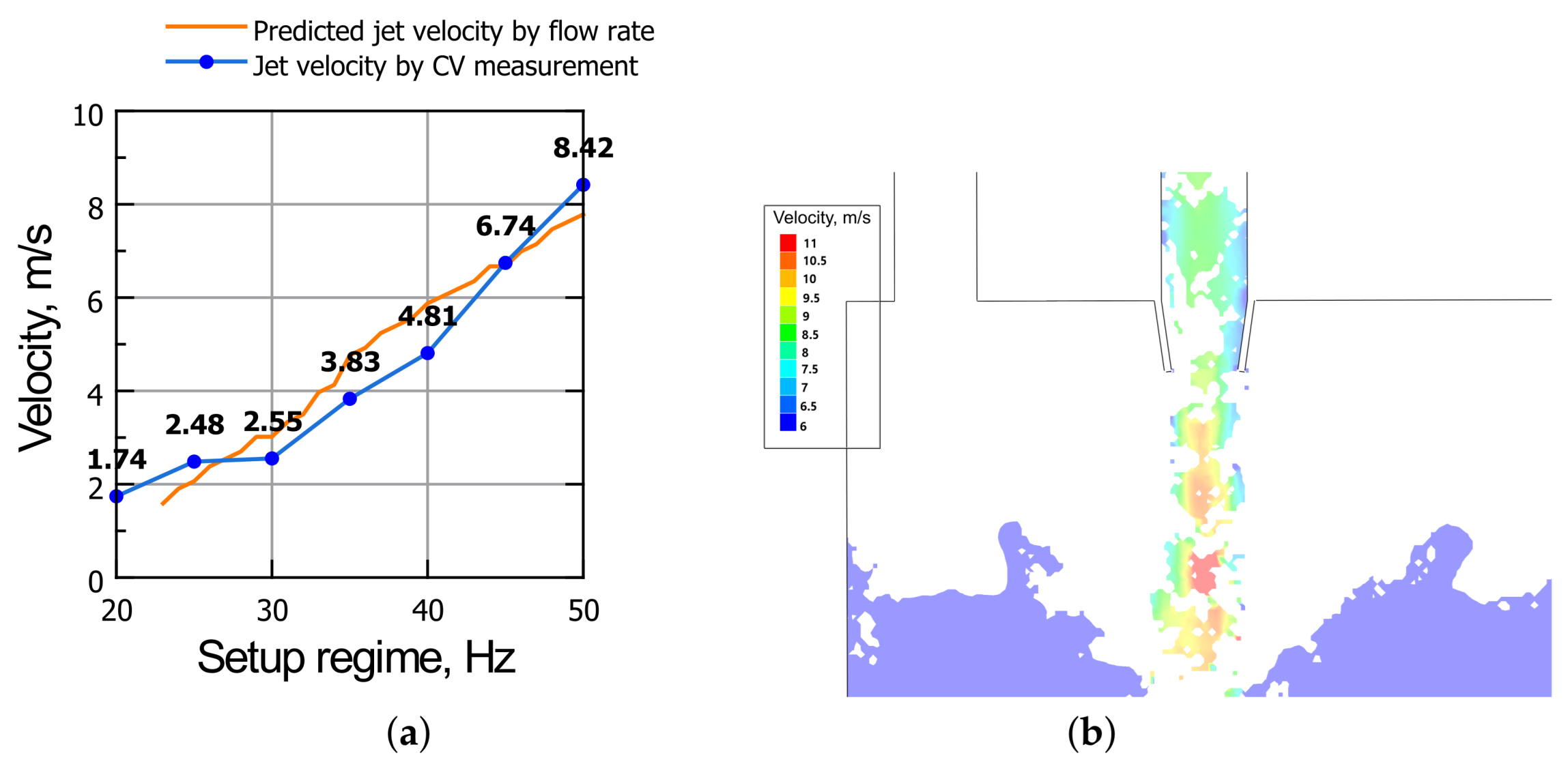
In Figure 17a, the average jet velocities measured with the proposed CV algorithm for each of the installation modes are presented (blue line). Note that for the 20–25 Hz modes with a split jet, the velocity values will be affected by the resistance of the gas phase to individual droplets. Therefore, it is expected that despite the growth in the liquid flow rate, the jet velocity grows slowly. As soon as the jet flow passes to the ring or continuous state (from 30 Hz), the velocity begins to grow almost linearly with the increase in liquid flow as the carrying phase. In the 40–50 Hz regimes, there is a decrease in the aerator ejection coefficient (Figure 11), which is an indication of insufficient gas phase inflow due to the design limitations of the aerator. At the same time, significant pressure and velocity pulsations may occur in the jet, which lead to an increase in the jet angle and deviation of the edge contour. In general, the jet velocity can be predicted from the balance of the liquid $Q_{liq}$ and gas $Q_{gas}$ flow rates. Since these flow rates are measured directly (see Figure 11), the velocity can be approximated as $\frac{Q_{gas}+Q_{liq}}{A_{nozzle}}$, where $A_{nozzle}$ is the nozzle cross-sectional area. This estimation is averaged over time and space and does not take into account the local influence of the wall roughness, bubble size, and structure on the hydraulic resistance of the flow. It also does not take into account the slip velocities between the bubbles and the fluid. Earlier, in work [13], it was shown that in a relevant bubble descent flow, the slip velocity can reach 10% of the liquid phase velocity. However, this is a good, physically reasonable approach for the verification of the computer vision method. Comparing the jet velocity from CV measurements and the predicted velocity based on the conservation principle (blue and orange curves in Figure 11), one can see a difference not exceeding 15%.

Earlier, CFD simulations using the FlowVision 3.09.05 software [53] of the jet flow in the unit were performed for the 50 Hz mode and showed liquid flow velocities from 8.5 m/s at the edges of the jet to 11 m/s in the center of the jet (see Figure 17b). Taking into account such a convex velocity profile, and the fact that the proposed computer vision method works only with the jet surface, we note the good correspondence of the obtained velocity measurement results with the results of CFD simulations.

These conclusions can be considered as verification of the developed algorithm.

Using the represented methodology, we were able to determine the optimal operating mode of the experimental setup in terms of maximizing the specific impulse per unit volume of the gas–liquid jet. This mode corresponds to the minimum jet angle and edge deviation and maximum flow velocity. In the case of industrial fermenters, the comparison of CV measurements and averaged predictions of gas and liquid flow rates at the aerator inlet allows the localization of anomalous modes of jet formation (e.g., due to design defects in the aerator or equipment wear during operation). The flexibility of the methodology that we propose is limited by the possibilities of verification. For each new jet stream apparatus, it is necessary to calibrate the computer vision method in order to obtain adequate results.

4. Conclusions

The methods of threshold segmentation, active contours, the regression of principal components, and the comparison of feature overlays made it possible to implement a scheme for the calculation of the jet stream angles, edge deviations, and velocities of gas–liquid jets for various video data and operating modes of the experimental setup.

The comparison of experimental data and modeling with computer vision calculations showed that the velocity estimates were close and the differences did not exceed 15%. Moreover, the CV measurements were consistent with third-party CFD calculations. At the same time, edge detection was found to be quite accurate and stable even with noisy data and a rough initial approximation in the form of a segment for all frames of one video recording. The comparison of the proposed algorithm with the results of partitioning using the classical Canny method yielded an RMS error of no more than 0.07 pixels. At the same time, the Canny method loses robustness when jet droplets break away and therefore requires resource-intensive image preprocessing. The proposed algorithm does not demonstrate this problem.

Test CV measurements have shown that the real jet in the apparatus may have asymmetric angles for the left and right boundaries. In addition, the environment inside the apparatus (foggy with high light scattering) leads to noise in the original data images. The robustness of the proposed algorithm allows us to handle such data while maintaining sufficient accuracy.

The presented algorithms for the evaluation of jet characteristics by computer vision methods based on high-speed video records currently have a number of limitations. First, the efficiency of the algorithms (in terms of accuracy and stability) depends on the quality of the original image. The presence of splashes, blur, low or uneven image contrast, and the excessive illumination of certain areas affects the accuracy of the final result. This leads to the need to carefully choose the video shooting point, the type of lighting (front or back), and its intensity. Image preprocessing methods also require further research. In particular, it is obvious that for the automatic selection of structures whose interframe shift is estimated in the flow velocity measurement algorithm, it is necessary to use an adaptive threshold during binarization, as well as histogram intensity equalization algorithms in the jet image region.

In addition, it was found that the jet structure, which depends on the gas content, local velocities, and bubble sizes, as well as aerator operation features, can significantly affect the flow velocity profile in the jet. When a flow core with significantly higher velocities is formed in the center of the jet rather than near the walls, the CV algorithm can significantly underestimate the velocity values compared to the average cross-sectional velocity value.

The absence of a dependency on hardware and software and the great potential for the optimization of the program code make it possible to use the proposed method “in real time”, directly during experiments and in industrial processes.