Approximate Closed-Form Solution of the Differential Equation Describing Droplet Flight during Sprinkler Irrigation

Abstract

Sprinkler irrigation is widely used in agriculture because it allows for rational use of water. However, it can induce negative effects of soil erosion and of surface waterproofing. The scholars of these phenomena use the numerical integration of the equation of motion, but if there was an analytical solution, the study would be facilitated, and this solution could be used as software for regulating sprinklers. Therefore, in this study, the solution of the differential equation of the flight of droplets produced by sprinklers in the absence of wind was developed. The impossibility of an exact analytical solution to the ballistic problem due to the variability of the drag coefficient of the droplets is known; therefore, to find the integrals in closed form, the following were adopted: a new formula for the drag coefficient; a projection of the dynamic’s equation onto two local axes, one tangent and one normal to the trajectory and some linearization. To reduce the errors caused by the latter, the linearization coefficients and their calculation formulas were introduced through multiple non-linear regressions with respect to the jet angle and the initial droplet speed. The analytical modeling obtained, valid for jet angles from 10° to 40°, was compared to the exact numerical solution, showing, for the total travel distance, a high accuracy with a mean relative error MRE of 1.8% ± 1.4%. Even the comparison with the experimental data showed high accuracy with an MRE of 2.5% ±1.1%. These results make the analytical modeling capable of reliably calculating the travel distance, the flight time, the maximum trajectory height, the final fall angle and the ground impact speed. Since the proposed analytical modeling uses only elementary functions, it can be implemented in PLC programmable logic controllers, which could be useful for controlling water waste and erosive effects on the soil during sprinkler irrigation.

1. Introduction

Sprinkler irrigation is widely used in agriculture because it allows a rational use of water. However, the high specific power (W m⁻²), a product of kinetic energy (J m⁻³) with an application rate (m³ s⁻¹ m⁻²) of water droplets impacting soil, is a factor to be controlled because it can induce the negative effects of soil erosion and surface sealing [1]. The landing angle of the droplets on the soil surface is also a factor to be controlled because low values induce the negative effects of soil erosion and surface sealing [1].

In recent years, scientific research in this area has been oriented towards study, mathematical modeling and experimentation to reduce the phenomena of soil sealing and erosion and to increase distribution uniformity. Hui et al. [1] studied the influence of low sprinkler pressure on soil erosion. Chen et al. [2] investigated erosion due to droplet kinetic energy for different soil types and indicated the importance of pressure, nozzle diameter and sprinkler spacing. Hui et al. [3], after confirming that the phenomenon of soil erosion depends more on the impact angle than on the kinetic energy of the droplets, identify low-pressure sprinklers as a possible solution. Zhu et al. [4] quantified the angle of impact on crops such as corn and the associated splash production resulting in soil erosion. Chen et al. [5] studied the influence of the kinetic energy of droplets produced by low-pressure sprinklers on soil erosion. Ge et al. [6] set up a method to evaluate the kinetic energy, the diameter of the droplets and the distribution of their speeds. Félix-Félix et al. [7] characterized the morphology and velocity of the droplets in the laboratory with the aim of improving sprinkler simulation models. Hua et al. [8] proposed three-dimensional mathematical modeling of sprinkler rainfall, based on numerically solved ballistics equations, to estimate the influence of rotation speed and performed an experimental verification of it.

In many of these works, it was necessary to use the differential equations of droplet motion, solved through numerical methods [9,10,11,12]. In fact, the numerical solution allows for the simulation of the characteristics of the droplet trajectory and, therefore, the total travel distance, the height of the trajectory, the flight time, the landing angle and the terminal velocity. The differential equations of droplet motion during sprinkler irrigation are derived from Newton’s second law of dynamics, in which the system of external forces applied to the droplet is equal to the product of mass and acceleration [13,14,15,16,17,18,19]. The forces applied are gravity, buoyancy and drag. While the first two are constant during the motion, the drag force depends on the droplet velocity with a complex and non-unique law: this is the reason why the exact closed-form solution of the droplet flight dynamic equations is impossible.

This is why the numerical solution is necessary; however, in the recent past, two proposals for approximate analytical solutions have been made. In the first proposal [20], the closed-form solution was possible because two simplifying hypotheses were adopted. The first was on the simplified formulation of the drag coefficient, while the second concerned the way to project the vector equation of dynamics onto the x and y axes, multiplying the drag force by ${\mathrm{c}\mathrm{o}\mathrm{s}}^2 \theta$ and by ${\mathrm{s}\mathrm{i}\mathrm{n}}^2 \theta$ instead of by $\cos \theta$ and by$\sin \theta$, respectively. These simplifications, on the one hand, had allowed an easy closed-form solution, but on the other, had led to a certain error then calculated by Yan et al. [21]. In the second proposal [22], the solution was obtained by imposing that the drag coefficient followed Stokes’ law, i.e., the drag force linear function of the droplet velocity. This hypothesis, on the one hand, allowed for easy analytical integration but, on the other hand, introduced an easily reliable error if one considers that Stokes’ law is valid for $0.1\le Re\le 2$ while during the motion of the droplets, the Reynolds number Re is many times higher than this range, often by two or three orders of magnitude.

Comparing the two methods of solving the equations of motion, the analytical one and the numerical one, the advantage of the closed-form solution is that this is a set of equations based on elementary functions (trigonometric, logarithmic and exponential) that can be solved in sequence and instantaneously, using a double dozen cells in a spreadsheet. A pocket scientific calculator can also be used. Furthermore, it must be considered that equations based on elementary functions can be implemented in PLC (programmable logic controller). This possibility is precluded by numerical integration methods and, furthermore, these methods are not instantaneous: for each condition to be analyzed, modern software requires, on average, tens of seconds of processing. Finally, software for numerical integration can have high investment costs.

Therefore, a closed-form solution of the droplet flight dynamic equation, approximated by minimizing errors, will be carried out through a series of measures: the development of a new single formula for the drag coefficient valid for the entire droplet flight; a projection of the dynamic equation onto two local axes, one tangent and one normal to the trajectory; some appropriate linearization [23] introducing linearization coefficients as a function of the jet angle and the initial speed, with formulas obtained through multiple non-linear regressions.

2. Materials and Methods

Section 2.1 is dedicated to the setting of the two flight differential equations, one for the ascending portion of the trajectory and one for the descending portion, and to their partially approximate analytical solution. The integration procedure of these two flight equations is long and divided into many steps and is reported to allow interested readers to follow the procedure and the phases dedicated to the approximations. Instead, readers interested only in the final equations to determine the geometric and dynamic values of the trajectories useful for the study and mitigation of the soil erosion phenomenon can find them grouped in Section 3.4, which follows. They are to be used on the spreadsheet or inserted into the PLC software, i.e., into the microprocessors that can be installed in the sprinklers for their adjustment aimed at mitigating soil erosion during irrigation. Section 2.2 is dedicated to the description of the exact numerical integration of the two flight equations. The exact results of the numerical integration constitute the benchmark to evaluate (Section 3.1) the accuracy of the results of the analytical modeling equations developed in Section 2.1 and summarized in Section 3.4.

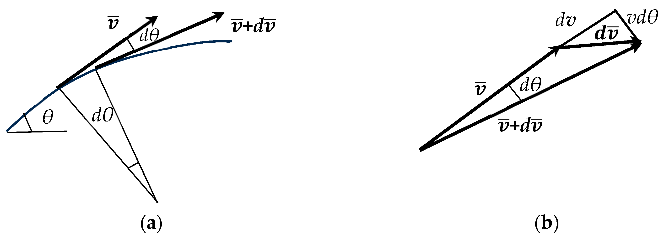
2.1. Closed-Form Solution and Mathematical Modeling

When the water jet comes out of the sprinkler nozzle, it is compact but then breaks into ligaments and then into droplets, thanks to the interaction with the ambient air. This is a complex phenomenon which also sees a subsequent interaction between the droplets themselves, already formed. As always happens in engineering, to study such a high complexity, some simplifying hypotheses [9] are posed to carry out mathematical modeling. If necessary, after comparing the solution and the experimental results, correction coefficients can be introduced.

Therefore, to set the differential equation of the flight of the droplets emitted from the nozzle, it was necessary to define some simplifying conditions:

• Flow of water completely disintegrates into droplets of various diameters in the outlet section of the sprinkler nozzle;
• All droplets have the same initial velocity, which is equal to the average velocity of the water flow in the exit section of the nozzle;
• Each droplet of water is considered alone along the trajectory, i.e., without collisions with the other droplets;
• Water droplets are considered rigid spheres upon exiting the nozzle and remain spherical during flight;
• Water droplets are not subject to evaporation, so their diameters remain unchanged throughout their trajectory;
• No wind.

Figure 1 shows the trajectory of a droplet emitted from the nozzle of a sprinkler.

It is possible to divide the trajectory into a first part from the emission point of the nozzle 0, which is at a height h (m) from the ground up to the top, and into a second part from the top up to the landing. The jet angle θ₀ (°) is the initial angle of the droplet jet, equal to the nozzle angle. The most important expected results of the mathematical modeling are the droplet travel distance x_tot (m), the flight time t_tot (s), the terminal velocity v_end (m s⁻¹) and the ground impact angle θ_end (°), which depend on droplet diameter D (m); initial velocity of the droplet v₀ (m s⁻¹); jet angle θ₀; nozzle height from the ground h (m); characteristics of air, such as viscosity μ (Pa s) and density ρ_air (kg m⁻³).

2.1.1. Ascending Portion of the Trajectory

Considering the ascending portion (Figure 1) from the sprinkler (0, h) to the top (x_top, y_top), the differential equation of dynamics is

$$m·\overline{a}=-m·\overline{g}-\overline{R}\to m_D·\frac{d\overline{v}}{dt}=-\left(m_D-m_{air}\right)·\overline{g}-c_d\frac{\pi }{4}{D}^2{\rho }_{air}\frac{v}{2}\overline{v}$$

(1)

where $\overline{a}=\frac{d\overline{v}}{dt}$ is the acceleration vector (m s⁻²), $m_D·\overline{g}$ is the gravitational force vector (N), m_D is the mass of the droplet (kg), $m_{air}·\overline{g}$ is the buoyancy force (N), m_air is the mass (kg) of the air moved by the droplet, $\overline{R}=c_d\frac{\pi }{4}{D}^2{\rho }_{air}\frac{v}{2}\overline{v}$ is the drag force vector (N), which is proportional to the drag coefficient c_d, to the equatorial area of the droplet of diameter D and to the kinetic energy (J). The air density is ρ_air (kg m⁻³). The buoyancy force is three orders of magnitude less than the gravitational force, so it can be neglected: $\left(m_D-m_{air}\cong m_D\right).$

Generally, to proceed with numerical integration and as was performed in a previous simplified analytical modeling [20], the vector Equation (1) is projected along the horizontal x and vertical y axes. Instead, in the present study, the projection of dynamics equation onto a local reference system having a tangent axis s and a normal axis n to the trajectory was chosen (Figure 2).

Figure 3 shows that the scalar velocity variation in the s direction is dv, and therefore, the acceleration is $\frac{dv}{dt}$, while in the n direction, the scalar velocity variation is v·dθ; therefore, the acceleration is $v\frac{d\theta }{dt}$. Therefore, Equation (1) projected onto s and n, neglecting the buoyancy force, which is three orders of magnitude less than the gravitational force $\left(m_D-m_{air}\cong m_D\right),$ becomes

$$\mathit{s}: m_D·\frac{dv}{dt}=m_D·\frac{d^{2}s}{{dt}^2}=-m_D·g·\mathrm{s}\mathrm{i}\mathrm{n}\theta -c_d\frac{\pi }{4}{D}^2{\rho }_{air}\frac{v^2}{2}$$

(2)

$$\mathit{n}: m_D·\frac{d\theta }{dt}v=m_D·g·\mathrm{c}\mathrm{o}\mathrm{s}\theta$$

(3)

The convention that the angle θ starts from the jet angle θ₀ value and takes on a positive value during the ascending portion of the trajectory is adopted.

In Equation (3), the component of the gravitational force has a positive sign because its direction is concordant with the n-axis. In Equation (2), the drag force appears in which the drag coefficient c_d is not constant but depends on the velocity v through the Reynolds number. Bird et al. (1960) [24] indicated that, with laminar motion $(0.1\le Re\le 2)$in the boundary layer, the Stokes formula $c_d=\frac{24}{Re}$ applies; with transition motion $(2<Re\le 500)$, the formula $c_d=\frac{18.5}{{Re}^{0.6}}$ applies; with turbulent motion $\left(Re>500\right)$, the formula $c_d=0.44$applies. These formulas are valid for rigid spheres.

Since, during the motion of the droplet, the Reynolds number varies, it may be that the choice of a relationship between the three indicated by Bird et al. [24] in order to perform the integration of Equation (2) produces important errors in the prediction of the droplet travel distance and the flight time.

To overcome this difficulty, in the present analytical model, a unique relationship has been applied. Recently [25], for$0.1\le Re\le \mathrm{200,000}$, the following formula was developed:

$c_d=26.31·{Re}^{-\left(0.000037447{·G}^4-0.00066989·G^3+0.0016779·G^2-0.033243·G+0.86961\right)},$ where$G=\mathrm{l}\mathrm{n}\left(Re\right).$ However, since in the motion of the droplets emitted by the sprinklers, the Reynolds number does not exceed the value of 10,000, the previous relationship has been simplified, always using the Standard Drag Curve data (SDC) [25,26]:

$$c_d=25.1·{Re}^{0.04925·\mathrm{l}\mathrm{n}Re-0.90977}$$

(4)

It is valid for $0.3\le Re\le \mathrm{10,000}$ and, compared to the SDC data, it has a relative mean error—MRE = 3.8% and a standard deviation—SD = 3.0%. In the same Reynolds range, the three relationships proposed by Bird et el. [24] present MRE = 3.1% and SD = 3.0%, i.e., values similar to those obtained with (4).

Equation (2) with (4), after dividing by the mass of the droplet m_D, becomes

$$\frac{dv}{dt}=\frac{dv}{d\theta }·\frac{d\theta }{dt}=-g·\mathrm{s}\mathrm{i}\mathrm{n}\theta -25.1·{Re}^{0.04925·\mathrm{l}\mathrm{n}Re-0.90977}·\frac{\pi }{8}{D}^2\frac{{\rho }_{air}}{m_D}{v}^2$$

(5)

Equation (3) gives $\frac{d\theta }{dt}=\frac{g}{v}·\mathrm{c}\mathrm{o}\mathrm{s}\theta$, which is inserted into (5). Furthermore, the velocity variable v is replaced with the Reynolds number variable Re, $v=Re\frac{\mu }{{\rho }_{air}·D}$, where μ is the air viscosity (Pa s). Finally, instead of the mass of the spherical droplet, the expression is inserted, $m_D={\rho }_w\frac{\pi D^3}{6}$, where ρ_w is the density of water (kg m⁻³). Equation (5) becomes

$$\frac{dRe}{d\theta }=-Re·\tan \theta -\frac{25.1}{Ar}·\frac{{Re}^{0.04925·\mathrm{l}\mathrm{n}Re-0.90977+3}}{\cos \theta }$$

(6)

where the quantity Ar is the Archimedes number [25]: $Ar=\frac{4}{3}\frac{D^3{\rho }_{air}\cdot {\rho }_w\cdot g}{{\mu }^2}$.

Equation (6) is a non-integrable differential equation due to the exponent $(0.04925·\mathrm{l}\mathrm{n}Re-0.90977+3)$. However, through some parallel numerical integration tests of Equation (6), it was seen that the maximum decrease in Re occurs with the minimum droplet diameter of 0.25 mm and is approximately 30-fold during the ascending part of the trajectory. Consequently, the maximum variation of the exponent $(0.04925·\mathrm{l}\mathrm{n}Re-0.90977+3)$ is 7%, while it reduces to 2% with large droplet diameter (D = 5 mm).

Consequently, the simplifying hypothesis of considering the exponent calculated with the Reynolds number equal to the initial value ${Re}_0=\frac{{\rho }_{air}{v}_{0}D}{\mu }$ was adopted. Therefore, Equation (6) becomes

$$\frac{dRe}{d\theta }=-Re·\tan \theta -\frac{25.1}{Ar}·\frac{{Re}^{\beta }}{\cos \theta }$$

(7)

where $\beta =0.04925·\mathrm{l}\mathrm{n}{Re}_0-0.90977+3$.

By introducing the new variable $u_a=\frac{1}{{Re}^{\beta -1}}$, so $\frac{d{u}_a}{d\theta }=\frac{-\left(\beta -1\right)}{{Re}^{\beta }}\frac{dRe}{d\theta }$, Equation (7) can be transformed:

$$\frac{{du}_a}{d\theta }=\left(\beta -1\right)·u_a·\tan \theta +\frac{\left(\beta -1\right)}{Ar}·\frac{25.1}{\cos \theta }$$

(8)

Equation (8) is a first-order linear differential equation that can be solved by the Bernoulli method, that is, by introducing the variable u_a as the product of two dummy variables w_a and z_a: $u_a=w_a·z_a$. Therefore, Equation (8) becomes

$$\frac{{dw}_a}{d\theta }{z}_a+w_a\frac{d{z}_a}{d\theta }=\left(\beta -1\right)·w_a·z_a·\tan \theta +\frac{\left(\beta -1\right)}{Ar}·\frac{25.1}{\cos \theta }$$

(9)

A function $z_a=z_a\left(\theta \right)$ must be found such that its derivative satisfies this equality:

$$w_a\frac{d{z}_a}{d\theta }=\left(\beta -1\right)·w_a·z_a·\tan \theta$$

(10)

It is sufficient to integrate, by separation of the variables, Equation (10) to obtain the desired function:

$$z_a=C_{za}·{\left(\cos \theta \right)}^{-\left(\beta -1\right)}$$

(11)

where C_za is the constant of integration. The combination of Equations (9)–(11) gives

$$\frac{{dw}_a}{d\theta }=\frac{\beta -1}{C_{za}}·\frac{25.1}{Ar}·\frac{{\left(\cos \theta \right)}^{\left(\beta -1\right)}}{\cos \theta }$$

(12)

Since β is between approximately 2.3 and 2.6 depending on the droplet diameter D and the initial velocity v₀, (β − 1) is between 1.3 and 1.6, i.e., non-integer number, so the differential equation (12) has no solution in closed form. However, the expression ${\left(\cos \theta \right)}^{\left(\beta -1\right)}$can be replaced by $\alpha {\left(\cos \theta \right)}^2$, where the coefficient α depends on the initial values of the Reynolds number Re₀, the jet angle θ₀ and the water pressure in the nozzle p. The relationship $\alpha =\alpha \left({Re}_0,{\theta }_0,p\right)$ will be obtained later, in Appendix A, using a nonlinear multiple regression. It will be performed in such a way as to also consider the errors due to the approximation introduced in Equation (7) with the exponent β = constant. Thus, Equation (12) becomes

$$\frac{{dw}_a}{d\theta }=\frac{\beta -1}{C_{za}}·\frac{25.1}{Ar}·\mathsf{\alpha }·\cos \theta$$

(13)

The solution of which, containing the quantity C_wa, which is the value assumed by the variable w_a when θ = θ₀, is

$$w_a=\frac{\beta -1}{C_{za}}·\frac{25.1}{Ar}·\alpha \left(\sin {\theta }_0-\sin \theta \right)+C_{wa}$$

(14)

Combining Equations (14) and (11), the variable u_a becomes

$$u_a=w_a·z_a=\frac{\left(25.1/Ar\right)·\left(\beta -1\right)·\alpha ·\left(\sin {\theta }_0-\sin \theta \right)+C_{ua}}{{\left(\cos \theta \right)}^{\beta -1}}$$

(15)

where $C_{ua}=C_{wa}·C_{za}$. Since $u_a={Re}^{-\left(\beta -1\right)},$ Equation (15) becomes

$$Re=\frac{\cos \theta }{{\left[\frac{25.1}{Ar}\left(\beta -1\right)·\alpha ·\left(\sin {\theta }_0-\sin \theta \right)+C_{ua}\right]}^{\frac{1}{\beta -1}}}$$

(16)

By imposing the initial conditions, $\theta ={\theta }_0, Re={Re}_0$, the constant C_ua is obtained, as follows:

$$C_{ua}={\left(\frac{\cos {\theta }_0}{{Re}_0}\right)}^{\beta -1}$$

(17)

Setting θ = 0, Equation (16) gives the value of the Reynolds number at the top of the trajectory:

$${Re}_{top}=\frac{1}{{\left[\frac{25.1}{Ar}\left(\beta -1\right)·\alpha ·\sin {\theta }_0+C_{ua}\right]}^{\frac{1}{\beta -1}}}$$

(18)

From Equation (16), it is easy to obtain the velocity of the droplet with diameter D:

$$v_a=\frac{d{s}_a}{dt}=\frac{\mu }{{\rho }_{air}D}·\frac{\cos \theta }{{\left[\frac{25.1}{Ar}\left(\beta -1\right)·\alpha ·\left(\sin {\theta }_0-\sin \theta \right)+C_{ua}\right]}^{\frac{1}{\beta -1}}}$$

(19)

The integral of Equation (19) provides the length s_a (m) of the trajectory in the ascending portion as a function of the time and angle θ:

$$s_a=\frac{\mu }{{\rho }_{air}D}\int \frac{\cos \theta ·dt}{{\left[\frac{25.1}{Ar}\left(\beta -1\right)·\alpha ·\left(\sin {\theta }_0-\sin \theta \right)+C_{ua}\right]}^{\frac{1}{\beta -1}}}$$

(20)

The combination of Equation (19) with the expression $\frac{d\theta }{dt}=\frac{g}{v}·\mathrm{c}\mathrm{o}\mathrm{s}\theta$ obtained from Equation (3) gives the elemental time interval dt as a function of angle θ:

$$dt=\frac{\mu }{{\rho }_{air}Dg}\frac{d\theta }{{\left[\frac{25.1}{Ar}\left(\beta -1\right)·\alpha ·\left(\sin {\theta }_0-\sin \theta \right)+C_{ua}\right]}^{\frac{1}{\beta -1}}}$$

(21)

Finally, the combination of Equations (20) and (21) gives s_a as a function of only the angle θ:

$$s_a=\frac{{\mu }^2}{{\rho }_{air}^2{D}^{2}g}\int \frac{\cos \theta ·d\theta }{{\left[\frac{25.1}{Ar}\left(\beta -1\right)·\alpha ·\left(\sin {\theta }_0-\sin \theta \right)+C_{ua}\right]}^{\frac{2}{\beta -1}}}$$

(22)

Performing the integral, Equation (22) becomes

$$s_a=\frac{{\mu }^2}{{\rho }_{air}^2{D}^{2}g}·\frac{\frac{25.1}{Ar}\alpha \left(\beta -1\right) \left(\sin \theta -\sin {\theta }_0\right)-C_{ua}}{\frac{25.1}{Ar}\alpha \left(3-\beta \right){\left[-\frac{25.1}{Ar}\alpha \left(\beta -1\right)\left(\sin \theta -\sin {\theta }_0\right)+C_{ua}\right]}^{\frac{2}{\beta -1}}}+C_s$$

(23)

where C_s is the constant of integration, which is determined by imposing the initial conditions $\theta ={\theta }_0, s_a=0$. Furthermore, by imposing $\theta =0$, Equation (23) gives the length of the ascending trajectory up to the top:

$$s_{top}=\frac{{\mu }^2}{{\rho }_{air}^2{D}^{2}g}\left\{\frac{-\frac{25.1}{Ar}\alpha \left(\beta -1\right)\sin {\theta }_0-C_{ua} }{\frac{25.1}{Ar}\alpha \left(3-\beta \right){\left[\frac{25.1}{Ar}\alpha \left(\beta -1\right)\sin {\theta }_0+C_{ua}\right]}^{\frac{2}{\beta -1}}}+\frac{{C_{ua}}^{\frac{\beta -3}{\beta -1}}}{\frac{25.1}{Ar}\alpha \left(3-\beta \right)}\right\}$$

(24)

If the function inside the integral of Equation (22) were multiplied by cos θ, the integration would provide the droplet travel distance x_top or, if it were multiplied by sin θ, the integration would provide the height y_top (Figure 1). Unfortunately, the two new functions cannot be integrated; therefore, simplified calculation methods of x_a and y_a are proposed. It is valid because it involves mean relative errors of approximately 1%. The variables s_a and, therefore, x_a and y_a of the ascending portion originate at the sprinkler nozzle (Figure 1).

The method consists of calculating the arithmetic mean value, γ, of cos θ₀ and cos 0, which is $\gamma =\frac{\cos {\theta }_0+1}{2}$, and multiplying it by s_a, obtaining the droplet travel distance x_top. To obtain y_top, first, the average angle θ_ave is calculated, then its trigonometric tangent is calculated, which is the ratio between y_top and x_top. The formulas are

$$\left\{\begin{array}{c}\gamma =\frac{\cos {\theta }_0+1}{2}\\ x_{top}=s_{top}·\gamma \\ {\theta }_{ave}=\arccos \gamma \\ y_{top}=x_{top}·\tan {\theta }_{ave}\end{array}\right.$$

(25)

To obtain the flight time to the top, Equation (21) could be used, which, however, cannot be integrated. However, with the precaution of multiplying the function inside the integral of Equation (21) by the $\cos \theta ,$ a solution is obtained, which must be corrected with a coefficient φ to be obtained (Appendix A) via the regression method, similar to the coefficient α. Therefore, the following equation gives the flight time t_top:

$$t_{top}=\phi \frac{\mu }{{\rho }_{air}Dg}\left\{\frac{-\frac{25.1}{Ar}\alpha \left(\beta -1\right)\sin {\theta }_0-C_{ua} }{\frac{25.1}{Ar}\alpha \left(2-\beta \right){\left[\frac{25.1}{Ar}\alpha \left(\beta -1\right)\sin {\theta }_0+C_{ua}\right]}^{\frac{1}{\beta -1}}}+\frac{{C_{ua}}^{\frac{\beta -2}{\beta -1}}}{\frac{25.1}{Ar}\alpha \left(2-\beta \right)}\right\}$$

(26)

2.1.2. Descending Portion of the Trajectory

The descending portion presents a differential equation of droplet motion like Equation (1), but with the difference that the sign of the gravitational force is positive because it becomes a driving force (Figure 1):

$$m_D·\frac{d\overline{v}}{dt}=\left(m_D-m_{air}\right)·\overline{g}-c_d\frac{\pi }{4}{D}^2{\rho }_{air}\frac{v}{2}\overline{v}$$

(27)

Therefore, Equation (7) also changes the sign as follows:

$$\frac{dRe}{d\theta }=Re·\tan \theta -\frac{25.1}{Ar}·\frac{{Re}^{\delta }}{\cos \theta }$$

(28)

where the exponent δ depends on the Reynolds number at the top of the trajectory Re_top, already determined by Equation (18): $\delta =0.04925·\mathrm{l}\mathrm{n}{Re}_{top}-0.90977+3$.

The convention is adopted that the angle θ starts from a zero value at the top of the trajectory and takes on a positive value during the descending portion.

Also, considering the dummy variable for the descending segment, $u_d=\frac{1}{{Re}^{\delta -1}}$ and $u_d{=w}_d·z_d$, Equations (9)–(12) become

$$\frac{{dw}_d}{d\theta }{z}_d+w_d\frac{d{z}_d}{d\theta }=-\left(\delta -1\right)·w_d·z_d·\tan \theta +\frac{\left(\delta -1\right)}{Ar}·\frac{25.1}{\cos \theta }$$

(29)

$$w_d\frac{d{z}_d}{d\theta }=-\left(\delta -1\right)·w_d·z_d·\tan \theta$$

(30)

$$z_d=C_{zd}·{\left(\cos \theta \right)}^{\left(\delta -1\right)}$$

(31)

$$\frac{{dw}_d}{d\theta }=\frac{\delta -1}{C_{zd}}·\frac{25.1}{Ar}·\frac{1}{{\left(\cos \theta \right)}^{\delta }}$$

(32)

Equation (32), like Equation (12), cannot be integrated because δ is not integer. But, even in this case, an approximation such as ${\left(\cos \theta \right)}^{\delta }\cong \epsilon {\left(\cos \theta \right)}^2$, where ε is a coefficient obtainable (Appendix A) through regression method like α, makes Equation (32) integrable, as follows:

$$\frac{{dw}_d}{d\theta }=\frac{\delta -1}{C_{zd}}·\frac{25.1}{Ar}·\frac{1}{{\epsilon \left(\cos \theta \right)}^2}$$

(33)

The solution is

$$w_d=\frac{\delta -1}{\epsilon ·C_{zd}}·\frac{25.1}{Ar}·\tan \theta +C_{wd}$$

(34)

where C_wd is the value of the variable w_d at the beginning of the descending trajectory, i.e., at the top when θ = θ_top = 0.

The multiplication of Equations (31) and (34) gives the dummy variable u_d relating to the descending section:

$$u_d{=w}_d·z_d=\left[\frac{\delta -1}{\epsilon }·\frac{25.1}{Ar}·\tan \theta +C_{ud}\right]{\left(\cos \theta \right)}^{\left(\delta -1\right)}$$

(35)

The new constant of the descending portion is $C_{ud}=C_{wd}{·C}_{zd}$. Since $u_d=\frac{1}{{Re}^{\delta -1}}$, Equation (35) becomes for the descending portion:

$$Re=\frac{{\rho }_{air}·v_d·D}{\mu }=\frac{1}{{\left[\frac{\delta -1}{\epsilon }·\frac{25.1}{Ar}·\tan \theta +C_{ud}\right]}^{\frac{1}{\delta -1}}\cos \theta }$$

(36)

The constant C_ud is determined with the initial condition of the descending portion: $\theta =0, Re={Re}_{top}$:

$$C_{ud}={\left(\frac{1}{{Re}_{top}}\right)}^{\delta -1}$$

(37)

From Equation (36), it is easy to obtain the elemental displacement ds_d of the droplet of diameter D along the descending portion of the trajectory:

$$d{s}_d=\frac{\mu }{{\rho }_{air}D}·\frac{dt}{{\left[\frac{\delta -1}{\epsilon }·\frac{25.1}{Ar}·\tan \theta +C_{ud}\right]}^{\frac{1}{\delta -1}}\cos \theta }$$

(38)

The combination of Equation (36) with the expression $\frac{d\theta }{dt}=\frac{g}{v}·\mathrm{c}\mathrm{o}\mathrm{s}\theta$, obtained from Equation (3), gives the following:

$$dt=\frac{\mu }{{\rho }_{air}Dg}·\frac{d\theta }{{\left[\frac{\delta -1}{\epsilon }·\frac{25.1}{Ar}·\tan \theta +C_{ud}\right]}^{\frac{1}{\delta -1}}{\left(\cos \theta \right)}^2}$$

(39)

By inserting Equation (39) into (38) and proceeding on to integration, the path length s_d(θ) of the droplet along the descending trajectory can be obtained:

$$s_d=\frac{{\mu }^2}{{\rho }_{air}^2{D}^{2}g}\int \frac{d\theta }{{\left[\frac{\delta -1}{\epsilon }·\frac{25.1}{Ar}·\tan \theta +C_{ud}\right]}^{\frac{2}{\delta -1}}{\left(\cos \theta \right)}^3}$$

(40)

Unfortunately, Equation (40) has no solution due to the term ${\left(\cos \theta \right)}^3$ and the non-integer exponent $\frac{2}{\delta -1}$. To overcome the first difficulty, (40) was projected onto the x-axis, given that the main objective is to have a formula for the droplet travel distance x. To overcome the second difficulty, a linearization was introduced:

$${\left[\tan \theta +\frac{\epsilon ·Ar·C_{ud}}{25.1\left(\delta -1\right)}\right]}^{\frac{2}{\delta -1}}\cong \lambda \left[\tan \theta +\frac{\epsilon ·Ar·C_{ud}}{25.1\left(\delta -1\right)}\right]+\eta$$

(41)

The coefficients λ and η will be determined using the regression method (Appendix A), as expected for the previous coefficients α, ε and φ. Equation (40) transforms as follows:

$$x_d=\frac{{\mu }^2}{{\rho }_{air}^2{D}^{2}g·\left(\frac{\delta -1}{\epsilon }·\frac{25.1}{Ar}\right)}\int \frac{d\theta }{{\left\{\lambda \left[\tan \theta +\frac{\epsilon ·Ar·C_{ud}}{25.1\left(\delta -1\right)}\right]+\eta \right\}\left(\cos \theta \right)}^2}$$

(42)

The variables x_d, y_d and s_d originate at the top of the trajectory (Figure 1).

The solution of Equation (42), including the constant of integration, is

$$x_d=\frac{1}{\lambda }\frac{{\mu }^2}{{\rho }_{air}^2{D}^{2}g·\left(\frac{\delta -1}{\epsilon }·\frac{25.1}{Ar}\right)}·\ln \left[\frac{\tan \theta +\frac{\epsilon ·Ar·C_{ud}}{25.1\left(\delta -1\right)}+\frac{\eta }{\lambda }}{\frac{\epsilon ·Ar·C_{ud}}{25.1\left(\delta -1\right)}+\frac{\eta }{\lambda }}\right]$$

(43)

For Equation (43) to provide the droplet travel distance x_d = x_end up to the point of impact to the ground, the landing angle of the trajectory at the point of impact θ_end must be known (Figure 1). An effective way to solve the problem is to start from the observation that the tan θ coincides with the derivative dy_d/dx_d. Therefore, it is sufficient to highlight the tan θ and proceed to the integration to obtain the coordinate y_d = y_d (x_d).

To facilitate the operation, some groups of parameters will be collected under two constant symbols, K₁ and K₂:

$$K_1=\frac{1}{\lambda }\frac{{\mu }^2}{{\rho }_{air}^2{D}^{2}g·\left(\frac{\delta -1}{\epsilon }·\frac{25.1}{Ar}\right)}$$

(44)

$$K_2=\frac{\epsilon ·Ar·C_{ud}}{25.1\left(\delta -1\right)}+\frac{\eta }{\lambda }$$

(45)

Thus, Equation (43) becomes

$$x_d=K_1·\ln \left[\frac{\tan \theta }{K_2}+1\right]$$

(46)

From which it is easy to highlight tan θ:

$$\tan \theta =\frac{d{y}_d}{d{x}_d}=K_2\left(e^{\frac{x_d}{K_1}}-1\right)$$

(47)

Integration of Equation (47) gives

$$y_d=K_2{K}_1\left(e^{\frac{x_d}{K_1}}-1\right)-K_2{x}_d$$

(48)

The combination of Equations (46) and (48) gives

$$y_d=K_1\tan \theta -K_2{K}_1·\ln \left[\frac{\tan \theta }{K_2}+1\right]$$

(49)

If this Equation (49) is applied to the landing point of the droplet, then the total height of the descending trajectory is known and equals ${y_{end}=y}_{top}+h$ (Figure 1), where y_top is obtained from Equation (25). Therefore, from (49), the only remaining unknown can be found: ${\theta =\theta }_{end}$.

With the value of θ_end entered into Equation (46), the complete travel distance of the descending portion x_end can be obtained. The total travel distance is the sum of the travel distance of the ascending portion x_top (25) and the descending portion x_end (46):

$$x_{tot}=x_{top}+x_{end}$$

(50)

Concerning the flight time during the descending trajectory, Equation (39) needs to be integrated. However, the exponent $\frac{1}{\delta -1}$ is not an integer and, therefore, prevents a solution. As already performed to solve Equation (40), a linearization is necessary:

$${\left[\tan \theta +\frac{\epsilon ·Ar·C_{ud}}{25.1\left(\delta -1\right)}\right]}^{\frac{1}{\delta -1}}\cong \sigma \left[\tan \theta +\frac{\epsilon ·Ar·C_{ud}}{25.1\left(\delta -1\right)}\right]+\psi$$

(51)

The coefficients σ and ψ will be determined using the regression method (Appendix A), as expected for the previous coefficients λ, η, α, ε and φ. Equation (39) transforms as follows:

$$t=\frac{\mu }{{\rho }_{air}Dg\left(\frac{\delta -1}{\epsilon }·\frac{25.1}{Ar}\right)}\int \frac{d\theta }{{\left\{\sigma \left[\tan \theta +\frac{\epsilon ·Ar·C_{ud}}{25.1\left(\delta -1\right)}\right]+\psi \right\}\left(\cos \theta \right)}^2}$$

(52)

After integrating (52) and entering the value of the landing angle $\theta ={\theta }_{end}$, the result obtained is the flight time from the top to the point of landing.

$$t_{end}=\frac{1}{\sigma }·\frac{\mu }{{\rho }_{air}Dg\left(\frac{\delta -1}{\epsilon }·\frac{25.1}{Ar}\right)}·\ln \left[\frac{\tan {\theta }_{end}+\frac{\epsilon ·Ar·C_{ud}}{25.1\left(\delta -1\right)}+\frac{\psi }{\sigma }}{\frac{\epsilon ·Ar·C_{ud}}{25.1\left(\delta -1\right)}+\frac{\psi }{\sigma }}\right]$$

(53)

Finally, the total flight time t_tot results from the sum of t_top (26) with t_end (53):

$$t_{tot}=t_{top}+t_{end}$$

(54)

2.2. Numerical Solution

The approximate closed-form solution, which led to the analytical modeling of the trajectory and, therefore, the travel distance, represented by Equations (18) for the calculation of Re_top, Equations (24) and (25) for the calculation of x_top and y_top, Equation (49) for the calculation of θ_end and Equation (46) for the calculation of x_end, was evaluated by comparing its results with the exact ones obtained with a numerical solution of the differential equation (ODE) of motion:

$$\frac{dRe}{d\theta }=-Re·\tan \theta -\frac{25.1}{Ar}·\frac{{Re}^{0.04925·\mathrm{l}\mathrm{n}Re-0.90977+3}}{\cos \theta }$$

(55)

This Equation (55) is that of the ascending portion of the trajectory and is different from Equation (7) because the variable exponent with ln Re has been kept, and therefore, it is the exact ODE. A similar differential equation was used for the descending portion of the trajectory. It also differs from Equation (28) because the variable exponent with ln Re has been maintained:

$$\frac{dRe}{d\theta }=Re·\tan \theta -\frac{25.1}{Ar}·\frac{{Re}^{0.04925·\mathrm{l}\mathrm{n}Re-0.90977+3}}{\cos \theta }$$

(56)

Both ODEs were integrated numerically for the first time to obtain Re as a function of θ. Finally, a subsequent numerical integration led to travel distance x and flight time t.

Numerical Adams’ method, especially suitable for this type of differential equation and easily implementable in Excel, was used for solving the two ODEs (55) and (56).

3. Results and Discussion

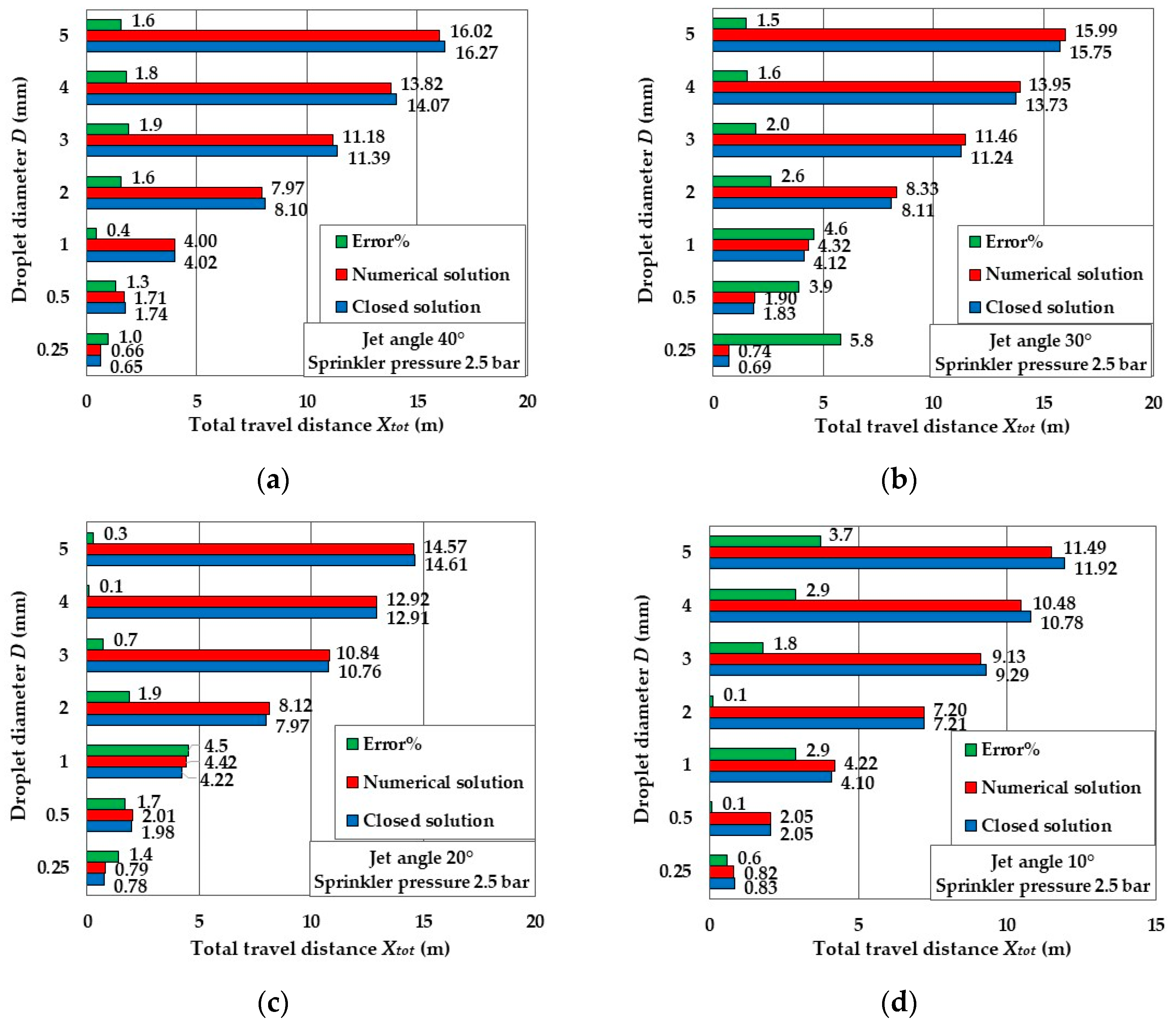
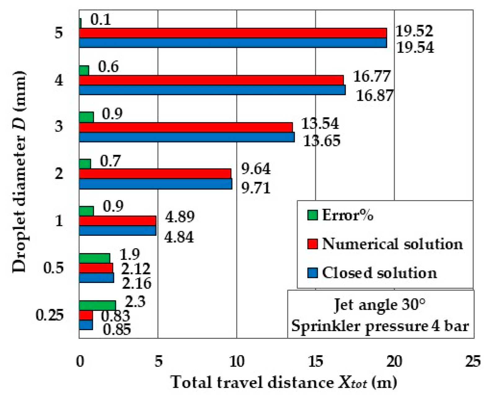
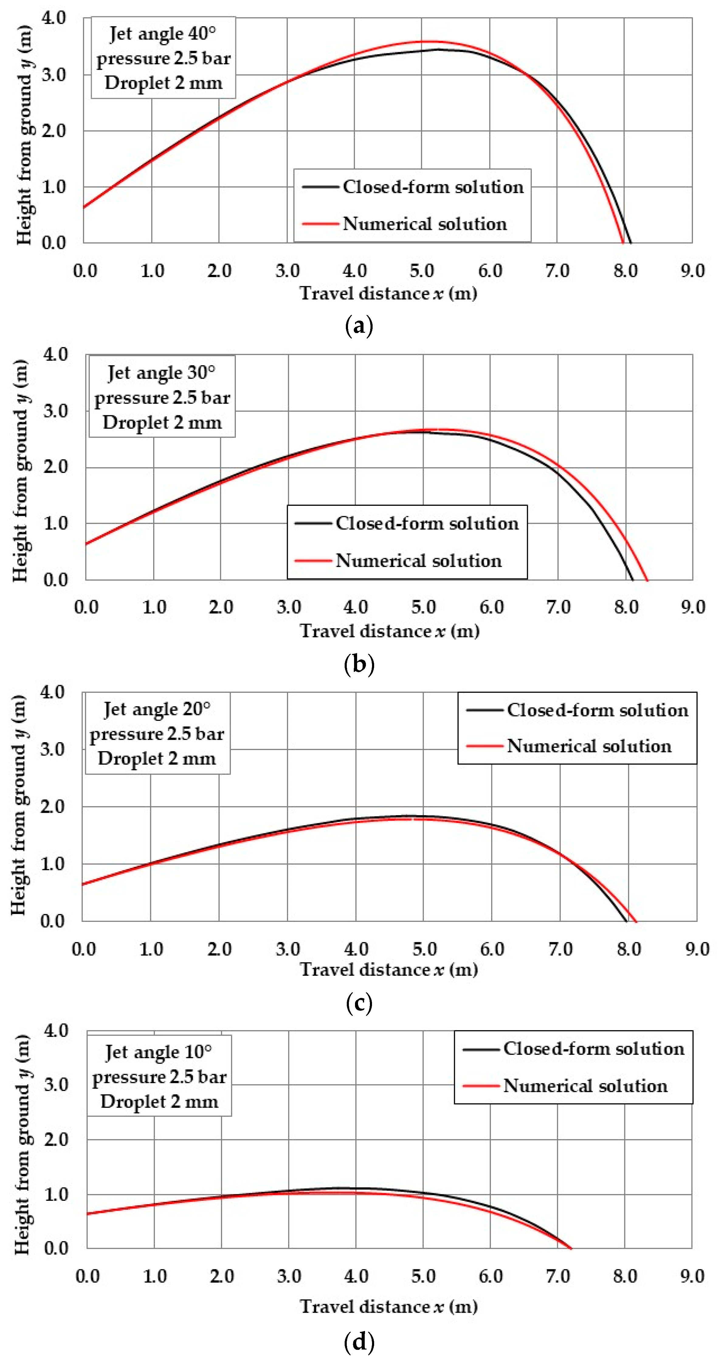
3.1. Comparison between Approximate Closed-Form Solution and Exact Numerical Solution

To evaluate the accuracy of the analytical modeling constituted by the approximate closed-form solution obtained in Section 2.1, the relevant equations to determine the travel distance were applied to droplets of seven different diameters (D = 0.25, 0.5, 1, 2, 3, 4 and 5 mm) produced by a sprinkler with different jet angles (θ₀ = 40°, 30°, 20° and 10°) and with two different pressures (p = 2.5 and 4 bar). The reference environmental conditions were air temperature T_air = 20 °C and altitude 50 m, which corresponded to air density ρ_air of 1.2 kg m⁻³ and air viscosity μ of 0.000018 Pa s.

With the same values of D, θ₀ and p, the numerical integrations described in Section 2.2 were carried out to obtain the exact values of the travel distance x_tot.

The comparison results are shown in Figure 4a–d, respectively, for each of the four jet angles θ₀ but with the same pressure p = 2.5 bar. To verify the accuracy of the approximate closed-form solution compared to the exact numerical one, with p = 4 bar, the numerical experimentation was limited to the variation of the diameter D, maintaining a single jet angle of 30°. The comparison results are shown in Figure 5.

The histograms of all the Figures show, through horizontal bars, the values of the travel distance x_tot obtained analytically (blue color) and numerically (red color) for each of the seven diameters of the droplet. In the histograms, for each diameter, there is a third bar (green color), which represents the relative percentage error, equal to

$$\mathrm{E}\mathrm{r}\mathrm{r}\mathrm{o}\mathrm{r}\mathrm{\%}=\left|\frac{{\left(x_{tot}\right)}_{analytic}-{\left(x_{tot}\right)}_{numeric}}{{\left(x_{tot}\right)}_{numeric}}\right|·100$$

(57)

Considering the set of 35 error% values, the mean relative error MRE is 1.8%, and the standard deviation SD is 1.4%. These values show how analytical modeling, i.e., based on the approximate closed-form solution, is a valid calculation tool.

To have a further qualitative evaluation of the accuracy of the approximate analytical solution compared to the exact numerical one, in Figure 6a–d, the trajectories were plotted and calculated both analytically and numerically with the four different jet angles (40°, 30°, 20° and 10°). The curves are limited to the case of the 2 mm droplet because, for other droplet diameters, the differences between the two trajectories are similar. These differences between the two trajectories, one calculated analytically (black line) and one calculated numerically (red line), confirm the relative error% calculated on the total travel distance, which was shown in Figure 4 and Figure 5.

For diameters less than approximately 0.45 mm, it may happen that the constant K₂ calculated with Equation (45) is negative, just below zero, due to the approximation of the values of the linearization coefficients introduced with the regression (Appendix A) of λ and η, despite R² = 0.99. This makes the solution of Equation (49) impossible because the argument of the logarithm function becomes negative.

The meaning of this event is that K₂ should tend to 0 due to the small size of the droplet and, therefore, its tendency to end its flight in a direction close to the vertical (${\theta }_{end}\to 90°)$, i.e., mathematically, the trajectory tends toward an asymptote. Therefore, for very small variations of θ_end, the variations of x_end are infinitesimal, but those of y_end become very large. This extreme situation would require absolute accuracy in the calculation of $K_2\to 0$, which the regression of λ and η cannot ensure. However, if (45) gives a negative K₂ just below zero, the difficulty is easily overcome by replacing this negative value with a positive K₂ value close to 0. Empirically, it has been found that the optimal value is K₂ = 10⁻⁴.

3.2. Comparison between Approximate Closed-Form Solution and Experimental Data

Analytical modeling based on the approximate closed-form solution was also applied to the experimentally measured droplet motion by Tompson et al. [27,28]. These authors measured the travel distance x_tot and the flight time t_tot for droplets with diameters D equal to 0.3, 0.9, 1.8, 3.0 and 5.1 mm emitted by a sprinkler with a jet angle θ₀ of 25° and with an initial velocity v₀ of 30.9 m/s. Nozzle height above ground h was 4.5 m and environmental conditions were air temperature T_air = 38 °C, relative humidity RH = 20% and no wind. Tompson’s experimental results compared to those of this study are shown in

Table 1. Total travel distance x_tot of sprinkler droplets: data of this study compared to those of Tompson et al. [27,28].

Droplet Diameter D (mm)	Travel Distance xtot (m) Tompson et al. [27,28]	Travel Distance xtot (m) This Study	Relative Error (%)
0.3	1.30	1.27	−2.6
0.9	5.22	5.20	−0.3
1.8	10.00	10.92	+9.2
3.0	13.48	17.27	+28.2
5.1	17.83	25.76	+44.5

and

Table 2. Total flight time t_tot of sprinkler droplets: data of this study compared to those of Tompson et al. [27,28].

Droplet Diameter D (mm)	Flight Time ttot (s) Tompson et al. [27,28]	Flight Time ttot (s) This Study	Relative Error (%)
0.3	2.63	1.03	−60.9
0.9	1.54	1.66	+7.7
1.8	1.63	1.97	+20.8
3.0	1.75	2.17	+24.1
5.1	1.84	2.38	+29.4

.

About the travel distance (Table 1), the mean relative error MRE is 17%, mainly due to a prediction of excessive travel distance x_tot for large droplets, from 3 to 5.1 mm.

For the flight time (Table 2), an MRE of 28% occurs due to the excessive time t_tot predicted by the analytical modeling for the larger droplets and a reduced t_tot for the 0.3 mm droplet.

3.3. Modification of the Drag Coefficient Formula to Consider the Deformation of the Droplets

Table 1 and Table 2 showed, in the case of medium and large droplets, too high values of the total travel distance and total flight time predicted by the analytical modeling. This is attributable to the reduced value of the drag coefficient obtained from Equation (4). In fact, it was obtained with a regression procedure starting from experimental data of the Standard Drag Curve (SDC) [25,26], which are valid for rigid spheres.

Yan et al. [21] and Kincaid [29], however, suggest using the approach of Park et al. [30,31], who, analyzing the data of Laws [32] and Gunn and Kinzer [33], found that the drag coefficient c_d for $Re\ge 1000$ begins to increase compared to the constant value of 0.44 due to the deformation of the droplets during flight.

The equation that Park et al. [30,31] suggested to take this fact into account is the following:

$$c_d=0.438·\left[1+0.021·{\left(\frac{Re}{1000}-1\right)}^{1.25}\right]$$

(58)

In this formula, there is a first constant term equal to 0.438, which is like the value of 0.44 predicted by Bird’s model [24] and 0.45 predicted by Fukui’s model [14]. Then, there is a second term in parentheses, which is a factor greater than 1 for $Re\ge 1000$. Due to this increasing factor, for example, with $Re=\mathrm{10,000}$, the drag coefficient c_d is 0.591.

In

Table 3. Drag coefficient c_d calculated with Equation (4), based on the Standard Drag Curve—SDC, introducing Re₀ of Tompson tests [27,28], compared with those calculated with Equation (58) of Park et al. [30,31].

Droplet Diameter D (mm)	Re0 Tompson et al. [27,28]	Drag Coefficient cd Equation (4) Based on SDC	Drag Coefficient cd Equation (58) Park et al. [30,31]
0.3	554	0.572	-
0.9	1661	0.442	0.443
1.8	3323	0.400	0.464
3.0	5538	0.383	0.499
5.1	9414	0.376	0.570

, the c_d values from Equations (4) and (58) have been compared considering the Reynolds numbers Re₀ of the experimental tests of Tompson et al. [27,28].

Table 3 shows that the values of Equation (4) are close to the experimental ones of the Standard Drag Curve—SDC [25,26], while those of Equation (58) are increasing with Re₀. The solution to this problem is to introduce the increasing factor present in the Equation (58) of Park et al. [30,31], also in Equation (4).

But Equation (58) has the term inside the brackets, which for $Re\le 1000$ cannot be calculated because it contains a negative number with a non-integer exponent, and in any case, the term in the brackets should remain constant and equal to 1. Therefore, a new empirical formula has been identified, which has a polynomial in place of the Park Equation (58), so that, for $Re\le 1000,$ Equation (4) remains valid, and for Re > 1000, it provides increasing values like those of Park. Ultimately, Formula (4), also considering the hypotheses written for Equation (7), becomes

$$\begin{gathered} c_d=\left[{0.000304\left(\frac{{Re}_0}{1000}\right)}^4-{0.00688\left(\frac{{Re}_0}{1000}\right)}^3+0.0499{\left(\frac{{Re}_0}{1000}\right)}^2-0.0637\left(\frac{{Re}_0}{1000}\right)+1.015\right] \\ ·25.1·{Re}^{0.04925·\mathrm{l}\mathrm{n}{Re}_0-0.90977} \end{gathered}$$

(59)

The new c_d values calculated with Equation (59) are, in the order of increasing D from 0.9 to 5.1 mm, 0.450, 0.456, 0.502 and 0.560. They differ from those obtained with Equation (58) of Park et al. (Table 3), with an MRE of only 1.5%. It must be noted that (58) is valid only for $1000\le Re\le \mathrm{10,000}$, while (59) is valid for $0.3\le Re\le \mathrm{10,000}$.

Formula (59) keeps expression (4) within it; therefore, the only modification to be made to the analytical modeling of Section 2.1. is to replace, in all the equations in which it is present, the number 25.1 with the constant K equal to

$$K=25.1·\left[{0.000304\left(\frac{{Re}_0}{1000}\right)}^4-{0.00688\left(\frac{{Re}_0}{1000}\right)}^3+0.0499{\left(\frac{{Re}_0}{1000}\right)}^2-0.0637\left(\frac{{Re}_0}{1000}\right)+1.015\right]$$

(60)

Because of this modification, the new values of total travel distance x_tot and total flight time t_tot are shown in

Table 4. Total travel distance x_tot of the droplets: data from the analytical modeling completed with Equation (60) of this study, compared to the experimental ones of Tompson et al. [27,28].

Droplet Diameter D (mm)	Travel Distance xtot (m) Tompson et al. [27,28]	Travel Distance xtot (m) This Study with Equation (60)	Relative Error (%)
0.3	1.30	1.27	−2.6
0.9	5.22	5.10	−2.4
1.8	10.00	9.60	−4.0
3.0	13.48	13.61	+1.0
5.1	17.83	18.23	+2.3

and

Table 5. Total flight time t_tot of sprinkler droplets: data of the analytical modeling completed with Equation (60), compared to those of Tompson et al. [27,28].

Droplet Diameter D (mm)	Total Flight Time ttot (s) Tompson et al. [27,28]	Total Flight Time ttot (s) This Study with Equation (60)	Relative Error (%)
0.3	2.63	1.03	−60.9
0.9	1.54	1.63	+5.8
1.8	1.63	1.85	+13.3
3.0	1.75	1.94	+11.0
5.1	1.84	2.01	+9.0

, respectively.

Table 4 shows the new travel distance values x_tot and the relative error% compared to Tompson’s experimental data. They are significantly better than those in Table 1. Now, the mean relative error MRE is 2.5%, and the standard deviation SD is 1.1%.

Therefore, the new values of c_d calculated with Equation (59), based on the indications of Park et al. [30,31], and the consequent replacement in the analytical model of Section 2.1. of the number 25.1 with the constant K of Equation (60), made the model capable of correctly describing the trajectory and therefore the total travel distance x_tot of the droplets experimentally analyzed by Tompson et al. [27,28].

Table 5 shows the new flight time values t_top. Excluding the flight time of the 0.3 mm droplet, the others were improved compared to those in Table 2. In particular, the mean relative error—MRE was 9.8%, and the SD was 3.2%.

The error of −60.9%, relating to the smallest droplet, seems to have no explanation. Perhaps the flight time was longer during the experimentation because the droplet was also involved, in the last part of the almost vertical trajectory, in a convective upward motion of the air due to temperature differences with the ground; very small mass of the droplet (14 μg); high height of the nozzle from the ground (4.5 m); final angle calculated with Equation (49) very high (θ₀ = 89.8°), which confirms a last part of the trajectory that is almost vertical.

3.4. Synoptic Table of the Definitive Analytical Modeling Based on Approximated Closed-Form Solution with the Drag Coefficient according to Park’s Values with Equations (59) and (60)

In this section, only the final equations of the closed-form integration carried out in Section 2.1 are collected, together with Equation (60) of Section 3.3 and the regression equations of Appendix A. They represent the mathematical model to be used on the spreadsheet or to be inserted into the PLC software (microprocessors dedicated to the control and regulation of sprinklers) to determine the geometric and dynamic values of the trajectories useful for the study and mitigation of the phenomena of soil sealing and erosion.

The travel distance of the ascending portion of the trajectory (0-top) is (Figure 1):

$$x_{top}=s_{top}·\gamma$$

(25a)

where

$$\gamma =\frac{\cos {\theta }_0+1}{2}$$

(25b)

$$s_{top}=\frac{{\mu }^2}{{\rho }_{air}^2{D}^{2}g}\left\{\frac{-\frac{K}{Ar}\alpha \left(\beta -1\right)\sin {\theta }_0-C_{ua} }{\frac{K}{Ar}\alpha \left(3-\beta \right){\left[\frac{K}{Ar}\alpha \left(\beta -1\right)\sin {\theta }_0+C_{ua}\right]}^{\frac{2}{\beta -1}}}+\frac{{C_{ua}}^{\frac{\beta -3}{\beta -1}}}{\frac{K}{Ar}\alpha \left(3-\beta \right)}\right\}$$

(24)

where the quantities K, Ar, β, α and C_ua are

$$K=25.1·\left[{0.000304\left(\frac{{Re}_0}{1000}\right)}^4-{0.00688\left(\frac{{Re}_0}{1000}\right)}^3+0.0499{\left(\frac{{Re}_0}{1000}\right)}^2-0.0637\left(\frac{{Re}_0}{1000}\right)+1.015\right]$$

(60)

$$Ar=\frac{4}{3}\frac{D^3{\rho }_{air}\cdot {\rho }_w\cdot g}{{\mu }^2}$$

(6)

$$\beta =0.04925·\mathrm{l}\mathrm{n}{Re}_0-0.90977+3$$

(7)

$$\alpha =\left(1.4677·{10}^{-6}{Re}_0{\theta }_0+7.7412·{10}^{-3}{\theta }_0+1.1394·{10}^{-5}{Re}_0+0.7516\right)·{\left(\frac{2.5}{p}\right)}^{0.01156·{Re}_0^{0.4}}$$

(A1)

$$C_{ua}={\left(\frac{\cos {\theta }_0}{{Re}_0}\right)}^{\beta -1}$$

(17)

where the initial value of Reynolds number (Figure 1) is ${Re}_0=\frac{{\rho }_{air}{v}_{0}D}{\mu }$.

The height from the nozzle to the top of the trajectory y_top is (Figure 1)

$$y_{top}=x_{top}·\tan {\theta }_{ave}$$

(25d)

where

$${\theta }_{ave}=\arccos \gamma$$

(25c)

The number of Reynolds at the top of trajectory Re_top is

$${Re}_{top}=\frac{1}{{\left[\frac{K}{Ar}·\left(\beta -1\right)·\alpha ·\sin {\theta }_0+C_{ua}\right]}^{\frac{1}{\beta -1}}}$$

(18)

The flight time from the nozzle to the top of the trajectory t_top is

$$t_{top}=\phi \frac{\mu }{{\rho }_{air}Dg}\left\{\frac{-\frac{K}{Ar}\alpha \left(\beta -1\right)\sin {\theta }_0-C_{ua} }{\frac{K}{Ar}\alpha \left(2-\beta \right){\left[\frac{K}{Ar}\alpha \left(\beta -1\right)\sin {\theta }_0+C_{ua}\right]}^{\frac{1}{\beta -1}}}+\frac{{C_{ua}}^{\frac{\beta -2}{\beta -1}}}{\frac{K}{Ar}\alpha \left(2-\beta \right)}\right\}$$

(26)

where

$$\phi =1.247·{\left(\cos {\theta }_0\right)}^{-0.5865}{·Re}_0^{-0.02691}$$

(A2)

The travel distance of the descending portion of the trajectory (top-end) is (Figure 1):

$$x_{end}=K_1·\ln \left[\frac{\tan \theta }{K_2}+1\right]$$

(46)

where the quantities K₁, K₂, δ, ε, λ, η and C_ud, are

$$K_1=\frac{1}{\lambda }\frac{{\mu }^2}{{\rho }_{air}^2{D}^{2}g·\left(\frac{\delta -1}{\epsilon }·\frac{K}{Ar}\right)}$$

(44)

$$K_2=\frac{\epsilon ·Ar·C_{ud}}{K·\left(\delta -1\right)}+\frac{\eta }{\lambda }$$

(45)

$$\delta =0.04925·\mathrm{l}\mathrm{n}{Re}_{top}-0.90977+3$$

(28)

$$\epsilon =0.966$$

(A3)

$$\lambda =8.748{·\theta }_0^{0.3179}{·\left(\ln {Re}_{top}\right)}^{-1.3454}$$

(A4)

$$\eta =0.115·{\theta }_0^{1.4321}·{Re}_{top}^{-0.3646}$$

(A5)

$$C_{ud}={\left(\frac{1}{{Re}_{top}}\right)}^{\delta -1}$$

(37)

The $\tan {\theta }_{end}$ can be obtained with an iterative method from the following:

$${y_{end}=y}_{top}+h=K_1\tan {\theta }_{end}-K_2{K}_1·\ln \left[\frac{\tan {\theta }_{end}}{K_2}+1\right]$$

(49)

The terminal velocity v_end is

$$v_{end}=\frac{\mu }{{\rho }_{air}D}·\frac{1}{{\left[\frac{\delta -1}{\epsilon }·\frac{K}{Ar}·\tan {\theta }_{end}+C_{ud}\right]}^{\frac{1}{\delta -1}}\cos {\theta }_{end}}$$

(36)

The total travel distance x_tot results from the sum of x_top (25a) and x_end (46):

$$x_{tot}=x_{top}+x_{end}$$

(50)

The flight time from top to end of the trajectory t_end is

$$t_{end}=\frac{1}{\sigma }·\frac{\mu }{{\rho }_{air}Dg\left(\frac{\delta -1}{\epsilon }·\frac{K}{Ar}\right)}·\ln \left[\frac{\tan {\theta }_{end}+\frac{\epsilon ·Ar·C_{ud}}{K·\left(\delta -1\right)}+\frac{\psi }{\sigma }}{\frac{\epsilon ·Ar·C_{ud}}{K·\left(\delta -1\right)}+\frac{\psi }{\sigma }}\right]$$

(53)

where

$$\sigma =1.2762{·\theta }_0^{-0.2312}·{Re}_{top}^{0.001854}$$

(A6)

$$\psi =0.0788·{\theta }_0^{0.3443}·{Re}_{top}^{0.05992}$$

(A7)

The total flight time t_tot is the sum of t_top (26) and t_end (51):

$$t_{tot}=t_{top}+t_{end}$$

(54)

The nomenclature of the quantities present in this Section 3.4 is collected in

Table 6. Nomenclature relating to the quantities of the equations in the synoptic table of definitive analytical modeling.

Symbol	Unity of Measurement	Description
a	m s−2	acceleration
Ar	-	Archimedes number
C	-	integration constant
cd	-	drag coefficient
D	m	droplet diameter
g	m s−2	gravity acceleration
h	m	nozzle height from the ground
m	kg	mass
n		axis normal to the trajectory
p	bar	nozzle pressure
Re	-	Reynolds number
s	m	axis tangential to the trajectory and/or length of the trajectory
t	s	time
v	m s−1	droplet velocity
u, w, z	-	auxiliary variables
x	m	travel distance
y	m	height of trajectory
Greek symbol	Unity of measurement	Description
α	-	linearization coefficient
β	-	Exponent in the drag coefficient formula for ascending trajectory
γ	-	linearization coefficient
δ	-	Exponent in the drag coefficient formula for descending trajectory
ε	-	linearization coefficient
η	-	“
θ	°	trajectory angle
λ	-	linearization coefficient
μ	Pa s	viscosity
ρ	kg m3	density
σ	-	linearization coefficient
φ	-	“
ψ	-	“
Subscript		Description
a		ascending portion of trajectory
air		air
ave		average
d		descending portion of trajectory
D		droplet
end		end of trajectory
top		top of trajectory
ua		integration constant of auxiliary variable u of ascending trajectory
ud		integration constant of auxiliary variable u of descending trajectory
w		water
0		start of trajectory

.

3.5. Results of the Application of Definitive Analytical Modeling

The definitive approximate analytical modeling, presented in the previous Section 3.4, was applied with the same diameters D (0.25, 0.5, 1, 2, 3, 4 and 5 mm) and with the same jet angles θ₀ (40°, 30°, 20° and 10°) and with the pressure p of 2.5 bar adopted during the comparison (Section 3.1) between the exact numerical solution and the approximate analytical one. For each diameter and for each jet angle, the result was the trajectories diagram (Figure 7a–d) and the total travel distance x_tot, the maximum height y_top, the impact angle on the ground θ_end and the terminal velocity v_end (

Table 7. Geometric and kinematic characteristics of droplet trajectories: total travel distance x_tot, maximum height from ground y_top + h, landing angle θ_end and terminal velocity at the landing v_end. Pressure p of 2.5 bar.

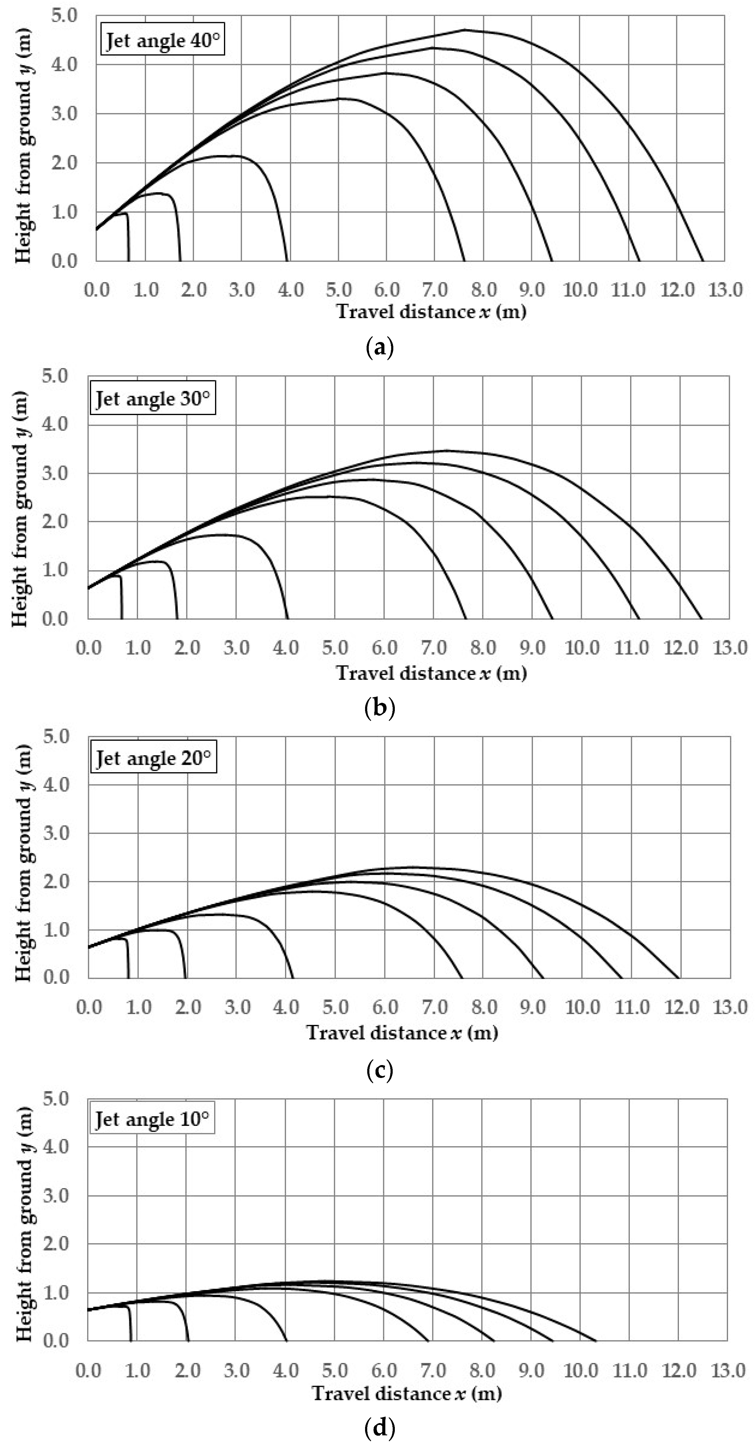
Jet Angle θ0 (°)	Droplet Diameter D (mm)	Travel Distance xtot (m)	Top Height from Ground ytop + h (m)	Landing Angl e θend (°)	Terminal Velocity vend (m/s)
	0.25	0.65	0.96	89.5	1.9
	0.5	1.73	1.37	87.2	3.2
	1	3.94	2.14	82.0	4.7
40°	2	7.62	3.30	75.0	6.4
	3	9.43	3.83	71.7	7.2
	4	11.24	4.34	69.0	7.9
	5	12.55	4.69	67.0	8.4
	0.25	0.69	0.88	89.4	1.8
	0.5	1.82	1.18	86.5	3.0
	1	4.05	1.72	79.5	4.3
30°	2	7.65	2.52	69.9	5.8
	3	9.43	2.88	65.4	6.5
	4	11.17	3.22	61.7	7.2
	5	12.44	3.46	59.2	7.7
	0.25	0.81	0.80	89.2	1.7
	0.5	1.97	1.00	85.3	2.8
	1	4.15	1.33	75.3	3.9
20°	2	7.57	1.79	61.1	5.3
	3	9.22	1.99	54.9	6.1
	4	10.80	2.17	50.1	6.8
	5	11.96	2.30	47.0	7.4
	0.25	0.87	0.73	88.7	1.6
	0.5	2.04	0.81	83.0	2.4
	1	4.04	0.94	66.9	3.3
10°	2	6.91	1.10	45.4	5.1
	3	8.25	1.16	37.6	6.2
	4	9.45	1.21	32.3	7.3
	5	10.32	1.25	29.2	8.2

).

Figure 7a–d, respectively, for the jet angles of 40°, 30°, 20° and 10°, each show the trajectories of the seven droplets differing in diameter, from 0.25 to 5 mm. Note that the total travel distances are smaller than those reported in Figure 4a–d due to the correction introduced with Equation (60), which is necessary to take into account the deformation of the larger droplets during the motion as predicted by Park et al. [30,31].

Finally, Table 7 shows the values of the total travel distance x_tot, obtained with Equation (50); of the maximum height y_top, obtained with (25d); of the landing angle θ_end, obtained with (49) and of the terminal velocity v_end, obtained with (36).

In the application of the definitive analytical model presented in Section 3.4, Figure 7 and, even more so, Table 7 show how the smallest jet angle (10°) has the smallest landing angles and quite high landing speeds. Scholars [1,2,3,4] point out that these values of the two parameters, the high dynamic one (landing velocity) and the low geometric one (landing angle), are the most dangerous for erosion and the formation of the superficial crust with relative reduction in infiltration. The travel distance achieved with a jet angle of 10° is also the lowest, therefore showing a lower efficiency in the use of irrigated water.

The largest landing angles, at less risk of erosion and the formation of surface crust, are obtained with jet angles of 40°. However, accepting a slight reduction in the landing angle but with an improvement in the travel distance and, above all, with a reduction in the landing velocity and, therefore, in the impact kinetic energy, the jet angle of 30° seems the most appropriate.

In any case, the application carried out here is limited to discrete jet angle values and, therefore, has only an example value. The reader will be able to carry out the application with different angles if they are within the 10–40° range.

As regards the influence of the diameter, Table 7 shows how the smaller droplets have much less impact and, therefore, are less dangerous for erosion and the formation of surface crust, both in terms of kinetic energy and landing angle.

3.6. Analytical Modeling and Droplet Evaporation

The analytical modeling summarized in Section 3.4 has, among the hypotheses, zero evaporation of the droplets during the flight. How far is this hypothesis from reality?

The results shown in Table 4, where the total travel distance calculated with the analytical modeling without evaporation are compared to the experimental one of Tompson et al. [27,28], where the droplets evaporated, highlights that the zero-evaporation hypothesis of the modeling is acceptable.

Confirmation can also be found in the experimentation and mathematical modeling of Kincaid and Longley [34]. They showed the influence of the droplet diameter D and environmental conditions (dry bulb temperature T_air and relative humidity RH%) on the loss rate of water mass through evaporation [35] during the flight.

The loss rate increases with increasing temperature, decreasing humidity and droplet diameter. The situation with the greatest loss rate occurred with the smallest droplet (D = 0.3 mm) and with the maximum temperature (T_air = 31 °C) and minimum humidity (RH = 22%). The loss rate was almost 10% s⁻¹, while, already with the droplet of 0.9 mm, the loss rate dropped to around 1.5% s⁻¹.

These are environmental conditions similar to those of the tests of Tompson et al. [27,28] (T_air = 38 °C and RH = 20%). Considering the droplet diameter D = 0.3 mm, the application of the loss rate of 10% s⁻¹, assumed constant during the entire flight time, which is approximately 1 s (Table 5), becomes a volume loss of the droplet of 10%. This volume reduction corresponds to a droplet diameter at the end of the flight equal to $D_{end}=\sqrt[3]{0.9}·D=0.29$ mm. With a constant loss rate, the average diameter during the flight is $D_{ave}=\left(D+D_{end}\right)/2=0.295$ mm. This is a reduction in diameter limited to 1.7%, which, applied to the mathematical modeling of paragraph 3.4, produces a new travel distance x_tot = 1.24 m compared to 1.27 m in Table 4. Clearly, this is an approximate procedure compared to the exact one, which should have used a new equation of motion with the presence of a dm/dt term.

The relative difference between 1.27 and 1.24 m is only −2.4%, which, with lower air temperatures and, above all, with higher humidity and larger diameters, becomes an imperceptible difference. It is concluded that the effects of evaporation on the travel distance calculated by the analytical modeling proposed here can be neglected without this worsening the predictive capacity of the modeling.

4. Conclusions

Starting from the differential equation of the flight of droplets emitted by sprinklers, its closed-form solution was studied through a new formulation of the drag coefficient; the projection of the vector equation onto two local axes, one tangent and one normal to the trajectory and some linearization. The linearization coefficients were obtained with multiple non-linear regressions as a function of the jet angle θ₀ and the initial velocity v₀. The set of equations obtained, presented in Section 3.4, is, therefore, an analytical model for droplet ballistics.

In a previous work from twenty years ago [20], the ballistics problem in terms of closed-form solution had already been studied. However, considering the simplifying hypotheses adopted at the time—particularly on the value of the drag coefficient and on the choice to write the projections on the x and y axes of the flight equation by multiplying the drag force by the ${\cos }^2\theta$ and ${\sin }^2\theta$, respectively, instead of $\cos \theta$ and $\sin \theta$—if, on the one hand, they allowed an easy closed-form solution, on the other, they introduced a mean relative error MRE that Yan et al. [21] calculated as equal to 42% compared to the experimental values of Tompson et al. [27,28]. Similar errors can be expected from the analytical integration proposal made by [22], in this case, due to the choice to formulate the drag coefficient via the Stokes equation.

Other authors in the last twenty years have studied the problem of droplet ballistics; however, they have always done so with the numerical solution of the differential equation of flight. The exact numerical solution was also performed in the present work but only to have a benchmark against which to evaluate the accuracy of the approximate closed-form solution proposed here.

The result of this comparison regarding the total travel distance was highly satisfactory, with a mean relative error MRE of 1.8% and a standard deviation SD of 1.4%.

Compared to the experimental data of Thompson et al. [27,28], the analytical model proposed here showed an MRE of 2.5% and an SD of 1.1%, confirming its high accuracy.

The proposed analytical modeling did not consider the mass loss due to evaporation, but the excellent fit with the experimental data of Thompson et al. [27,28], where the droplets evaporated, confirms what emerged in the Kincaid and Langley experiment [34]. These authors, in fact, had demonstrated that only very small droplets, when in environmental conditions of low humidity and high temperature, are subject to significant mass losses during flight, with values which, for these extreme cases, are, in any case, no higher than 10%.

The analytical modeling was built for a range of jet angle values between 10° and 40°; therefore, outside of it, the use of the model could lead to important errors.

Ultimately, the proposed analytical modeling is reliable and can predict, in the absence of wind, the travel distance, the maximum height of the trajectory, the landing angle and the terminal velocity before impact on the ground. This is all useful information for controlling water waste and the erosive effects on the soil due to the kinetic energy and landing angle of the droplets.

Furthermore, the proposed analytical modeling contains only elementary functions such as trigonometric ones, the logarithm and the exponential, which allow it to easily become the software for PLC control systems to be applied to sprinklers. In the future, it will, therefore, be interesting to verify the application to sprinkler irrigation systems of PLC-based hardware implemented with software attributable to this analytical modeling, which should also be expanded to consider the effects of the wind.

References

- Hui, X.; Zhao, H.; Zhang, H.; Wang, W.; Wang, J.; Yan, H. Specific power or droplet shear stress: Which is the primary cause of soil erosion under low-pressure sprinklers? Agric. Water Manag. 2023, 286, 108376. [Google Scholar] [CrossRef]
- Chen, R.; Li, H.; Wang, J.; Song, Z. Critical factors influencing soil runoff and erosion in sprinkler irrigation: Water application rate and droplet kinetic energy. Agric. Water Manag. 2023, 283, 108299. [Google Scholar] [CrossRef]
- Hui, X.; Zheng, Y.; Muhammad, R.S.; Tan, H.; Yan, H. Non-negligible factors in low-pressure sprinkler irrigation: Droplet impact angle and shear stress. J. Arid Land 2022, 14, 1293–1316. [Google Scholar] [CrossRef]
- Zhu, Z.; Zhu, D.; Ge, M. The spatial variation mechanism of size, velocity, and the landing angle of throughfall droplets under maize canopy. Water 2021, 13, 2083. [Google Scholar] [CrossRef]
- Chen, R.; Li, H.; Wang, J.; Guo, X. Analysis of droplet characteristics and kinetic energy distribution for fixed spray plate sprinkler at low working pressure. Trans. ASABE 2021, 64, 447–460. [Google Scholar] [CrossRef]
- Ge, M.; Wu, P.; Zhu, D.; Zhang, L. Analysis of kinetic energy distribution of big gun sprinkler applied to continuous moving hose-drawn traveler. Agric. Water Manag. 2018, 201, 118–132. [Google Scholar] [CrossRef]
- Félix-Félix, J.R.; Salinas-Tapia, H.; Bautista-Capetillo, C.; Garcia-Aragon, J.; Burguete, J.; Playan, E. A modified particle tracking velocimetry technique to characterize sprinkler irrigation drops. Irrig. Sci. 2017, 35, 515–531. [Google Scholar] [CrossRef]
- Hua, L.; Li, H.; Bortolini, L.; Jiang, Y. A model for predicting effects of rotation variation on water distribution of rotary sprinkler. Irrig. Sci. 2023, in press. [CrossRef]
- Zerihun, D.; Sanchez, C.A.; Warrick, A.W. Sprinkler irrigation droplet dynamics. I: Review and theoretical development. J. Irrig. Drain. Eng. 2016, 142, 04016007. [Google Scholar] [CrossRef]
- Zerihun, D.; Sanchez, C.A.; Warrick, A.W. Sprinkler irrigation droplet dynamics. II: Numerical solution and model evaluation. J. Irrig. Drain. Eng. 2016, 142, 04016008. [Google Scholar] [CrossRef]
- Zhang, R.; Liu, Y.; Zhu, D.; Wu, P.; Zheng, C.; Zhang, X.; Khudayberdi, N.; Liu, C. Simulating droplet distribution characteristics for sprinkler irrigation with a modified ballistic model. Comput. Electron. Agric. 2023, 215, 108437. [Google Scholar] [CrossRef]
- Zhang, R.; Liu, Y.; Zhu, D.; Zhang, X.; Gao, F.; Zheng, C. Modelling the spray range of rotating nozzles based on modified ballistic trajectory equation parameters. Irrig. Drain. 2023, 72, 343–357. [Google Scholar] [CrossRef]
- Seginer, I. Tangential velocity in sprinkler drops. Trans. ASAE 1965, 8, 90–93. [Google Scholar] [CrossRef]
- Fukui, Y.; Nakanish, K.; Okamura, S. Computer evaluation of sprinkler irrigation uniformity. Irrig. Sci. 1980, 2, 23–32. [Google Scholar] [CrossRef]
- von Bernuth, R.D.; Gilley, J.R. Sprinkler droplet size distribution estimation from single leg test data. Trans. ASAE 1984, 27, 1435–1441. [Google Scholar] [CrossRef]
- Vories, E.D.; Von Bernuth, R.D.; Mickelson, R.H. Simulating sprinkler performance in wind. J. Irrig. Drain. Eng. 1987, 113, 119–130. [Google Scholar] [CrossRef]
- Seginer, I.; Nir, D.; von Bernuth, R.D. Simulation of wind distorted sprinkler patterns. J. Irrig. Drain. Eng. 1991, 117, 285–306. [Google Scholar] [CrossRef]
- Carrion, P.; Tarjuelo, J.M.; Montero, J. SIRIAS: A simulation model for sprinkler irrigation. I: Description. Irrig. Sci. 2001, 20, 73–84. [Google Scholar] [CrossRef]
- Playan, E.; Burguete, J.; Zapata, N.; Salvador, R.; Bautista-Capetillo, C.; Cavero, J.; Martinez-Cob, A.; Faci, J.; Dechimi, F. Mathematical Problems and Solutions in Sprinkler Irrigation; Monografıas de la Real Academia de Ciencias 31: Zaragoza, Spain, 2009; pp. 153–174. [Google Scholar]
- Lorenzini, G. Simplified modelling of sprinkler droplet dynamics. Biosyst. Eng. 2004, 87, 1–11. [Google Scholar] [CrossRef]
- Yan, H.J.; Bai, G.; He, J.Q.; Li, Y.J. Model of droplet dynamics and evaporation for sprinkler irrigation. Biosyst. Eng. 2010, 106, 440–447. [Google Scholar] [CrossRef]
- Ben Charfi, I.; Corbari, C.; Skokovic, D.; Sobrino, J.; Mancini, M. Modeling of water distribution under center pivot irrigation technique. J. Irrig. Drain. Eng. 2021, 147, 04021024. [Google Scholar] [CrossRef]
- Friso, D. A new mathematical model for food thermal process prediction. Modell. Simul. Eng. 2013, 2013, 569473. [Google Scholar] [CrossRef]
- Bird, R.B.; Steward, W.E.; Lightfoot, E.N. Transport Phenomena; Wiley & Sons: New York, NY, USA, 1960; pp. 185–187. [Google Scholar]
- Friso, D. Mathematical modelling of particle terminal velocity for improved design of clarifiers, thickeners and flotation devices for wastewater treatment. Clean Technol. 2023, 5, 921–933. [Google Scholar] [CrossRef]
- Lapple, C.E.; Shepherd, C.B. Calculation of particle trajectories. Ind. Eng. Chem. 1940, 32, 605–617. [Google Scholar] [CrossRef]
- Thompson, A.L.; Gilley, J.R.; Norman, J.M. A sprinkler water droplet evaporation and plant canopy model: I Model development. Trans. ASAE 1993, 36, 735–741. [Google Scholar] [CrossRef]
- Thompson, A.L.; Gilley, J.R.; Norman, J.M. A sprinkler water droplet evaporation and plant canopy model: II. Model application. Trans. ASAE 1993, 36, 743–750. [Google Scholar] [CrossRef]
- Kincaid, D.C. Spray drop kinetic energy from irrigation sprinklers. Trans. ASAE 1996, 39, 847–853. [Google Scholar] [CrossRef]
- Park, S.W.; Mitchell, J.K.; Bubenzer, G.D. Splash erosion modeling: Physical analysis. Trans. ASAE 1982, 25, 357–361. [Google Scholar] [CrossRef]
- Park, S.W.; Mitchell, J.K.; Bubenzer, G.D. Rainfall characteristics and their relation to splash erosion. Trans. ASAE 1983, 26, 795–804. [Google Scholar] [CrossRef]
- Laws, J.O. Measurements of the fall velocity of waterdrops and raindrops. Trans. Am. Geophys. Union 1941, 22, 709–721. [Google Scholar] [CrossRef]
- Gunn, R.; Kinzer, G.D. The terminal velocity of fall for water droplets in stagnant air. J. Meteorol. 1949, 6, 243–248. [Google Scholar] [CrossRef]
- Kincaid, D.C.; and Longley, T.S. A water droplet evaporation and temperature model. Trans. ASAE 1989, 32, 457–462. [Google Scholar] [CrossRef]
- Friso, D. Conveyor-belt dryers with tangential flow for food drying: Mathematical modelling and design guidelines for final moisture content higher than the critical value. Inventions 2020, 5, 22. [Google Scholar] [CrossRef]