Machine Learning and Signal Processing for Bridge Traffic Classification with Radar Displacement Time-Series Data

Abstract

This paper introduces a novel nothing-on-road (NOR) bridge weigh-in-motion (BWIM) approach with deep learning (DL) and non-invasive ground-based radar (GBR) time-series data. BWIMs allow site-specific structural health monitoring (SHM) but are usually difficult to attach and maintain. GBR measures the bridge deflection contactless. In this study, GBR and an unmanned aerial vehicle (UAV) monitor a two-span bridge in Germany to gather ground-truth data. Based on the UAV data, we determine vehicle type, lane, locus, speed, axle count, and axle spacing for single-presence vehicle crossings. Since displacement is a global response, using peak detection like conventional strain-based BWIMs is challenging. Therefore, we investigate data-driven machine learning approaches to extract the vehicle configurations directly from the displacement data. Despite a small and imbalanced real-world dataset, the proposed approaches classify, e.g., the axle count for trucks with a balanced accuracy of 76.7% satisfyingly. Additionally, we demonstrate that, for the selected bridge, high-frequency vibrations can coincide with axles crossing the junction between the street and the bridge. We evaluate whether filtering approaches via bandpass filtering or wavelet transform can be exploited for axle count and axle spacing identification. Overall, we can show that GBR is a serious contender for BWIM systems.

1. Introduction

Extracting vehicle configurations on bridges is essential, like detecting overweight trucks and acquiring site-specific traffic information. This information can be considered for structural health monitoring (SHM). At an early stage of weight control, static scales have been used. However, the weighing process takes a long time, and measurement stations can be easily bypassed. An alternative approach uses sensors on the pavement that acquire dynamic measurements. This approach reduces the weighing time, but the sensors are exposed to more stress, making the system maintenance difficult. Current solutions use the bridge as a weighing scale [1,2,3]. These systems are called bridge weigh-in-motion (BWIM). A part of the bridge, such as the girder, is usually used to measure strain or acceleration during a vehicle crossing, which is henceforth referred to as an event. Axle count, spacing, and driving speed information determine the vehicle’s weight. Pavement sensors are generally exploited to acquire these three parameters. Nothing-on-road (NOR) BWIMs are entirely dispensed with pavement sensors by only using the lower side of the bridge for sensor attachment. This setup increases the challenge of acquiring data about the vehicle configuration. Also, the lower bridge side has to be accessible, which is not always the case. A remote NOR BWIM has barely been studied, except by Ojio et al. [3], who use cameras for contactless measurements.

Ground-based radar (GBR) has frequently been investigated in the context of bridge monitoring in recent years [4,5,6,7,8]. It achieves comparable or even better accuracy than established, conventional strain, or acceleration sensors [7] with the advantage of being remote and non-invasive. Thus, GBRs can be quickly set up for measurements. As they measure the bridge deflection and displacement, it can be directly applied to many SHM methods, like determining the dynamic input factor [9]. Furthermore, GBR has been investigated regarding the detection of bridge crossing events and, to some extent, the vehicle type classification [10,11]. Arnold and Keller [12] show that it is possible to differentiate between single- and multi-presence events from GBR deflection using machine learning (ML) despite facing challenges like variable-length time series and dataset imbalance. Yet, GBR has never been explicitly studied in the context of BWIM. In this paper, we will investigate the potential of GBR bridge displacement time series for BWIM by applying standard signal processing methods such as bandpass filtering and continuous wavelet transform (CWT) and using data-driven ML.

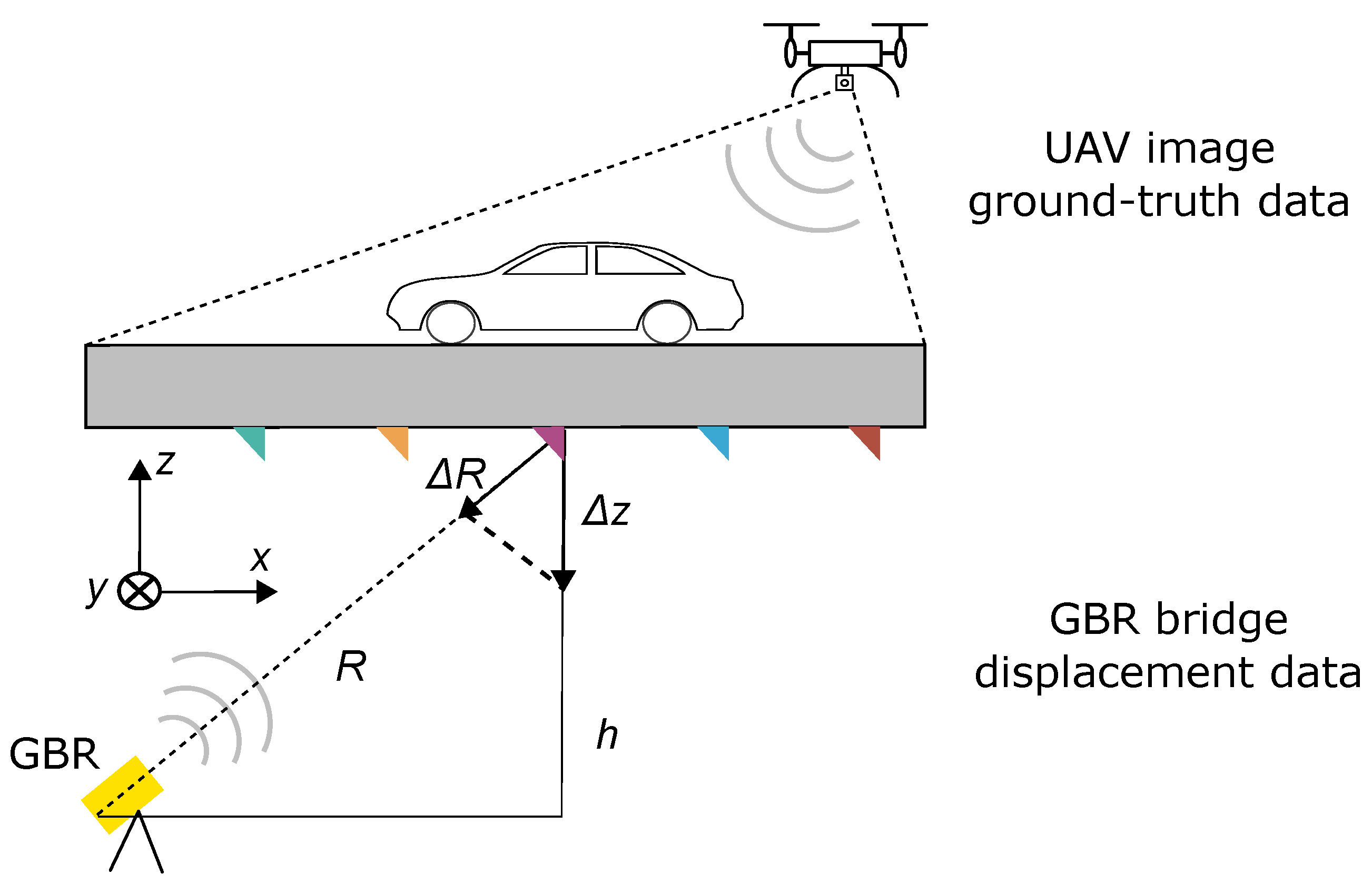
Our study is motivated by using remote displacement measurements with GBR in the context of BWIM. We develop an output-only method using GBR for analysis and an unmanned aerial vehicle (UAV) to gather ground-truth data. Measuring the displacement is challenging, so it has barely been studied for BWIM. Yet, it is regarded as a relevant feature for SHM [13]. To our knowledge, to this date, no study exists that tries to extract traffic information from only real-world bridge deflection. Since GBR-based bridge monitoring has many advantages, such a system would be beneficial. Therefore, we focus on two objectives.

• We analyze and implement ML approaches to determine relevant BWIM vehicle configurations, including vehicle type, lane, locus, speed, axle count, and spacing.
• We investigate signal processing techniques in the context of axle-related parameters.

An important aspect of BWIM is the determination of the traffic load. This study will not investigate load estimation since we do not have ground-truth data. However, Ojio et al. [3] showed that it is possible to extract the vehicle load from bridge displacement data. Furthermore, our approach is currently limited to single-vehicle events. Otherwise, the number of vehicles during an event has to be extracted from bridge displacement data. To date, no study in this regard has been conducted. Therefore, events during which multiple vehicles are present simultaneously have been discarded as Arnold and Keller [12] indicates that data-driven differentiation between single- and multi-presence events is possible.

First, we describe the related work relevant to this study in Section 2. In Section 3, we explain the setup for GBR measurements and describe the used dataset. In Section 4, we first cover the basics of wavelet transform. Then, the proposed feature extraction, the ML models, and the methodology for each task are detailed. The results of our approach are laid out in Section 5, and a comprehensive discussion is given in Section 6. Finally, Section 7 summarizes the main findings of this study.

2. Related Work

The relevance of time-series data in ML has never measured up to the prominence of images, although the variety in the data poses an exciting challenge. A wide range in scaling, length, sampling frequency, channels, etc., makes it challenging to develop versatile models to handle such complexity. The UCR dataset provides extensive datasets and is often used as a benchmark for new approaches [14]. However, at the date of writing this paper, only six datasets are both multi-variate and of unequal length. Moreover, the differences in signal length are minor. Oftentimes, an unequal length is circumvented by rescaling or padding in the time domain or extracting features, for instance, by fitting an autoregressive integrated moving average model [15]. Utilizing the UCR dataset, ref. [16] gives a detailed overview of the most relevant state-of-the-art methods for time-series classification. Random convolutional kernel transform (ROCKET), introduced by [17], is highlighted due to its training speed and as it has the best results, especially for multi-variate time-series classification. ROCKET uses random convolutional kernels to extract features, which are then used as input data for a linear ridge classifier. Dempster et al. [18] further refined ROCKET to a version called MiniRocket. MiniRocket is faster than ROCKET and is mostly deterministic while achieving comparable results. The authors also contributed a version of MiniRocket to the Python library sktime [19], which can handle unequal-length time series. Ref. [20] took an approach based on convolutional neural networks (CNNs) in combination with padding and masking for acoustic scene classification. To this end, they implemented a global pooling layer that supports masking to prevent the model from learning the padding. Arnold and Keller [12] used hand-crafted features for tree-based learners and MiniRocket for a bridge event classification on variable-length GBR displacement data. Additionally, they investigated the potential of data augmentation in this context. Overall, they achieve a balanced accuracy of over 90% when classifying crossings in single- or multi-presence events.

Several studies used ML or deep learning (DL) methods to extract vehicle information from NOR BWIM time series data. Kawakatsu et al. [21] attached a single strain sensor to the span of a 300 $\mathrm{m}$ long-concrete bridge in Japan. They used CNNs to detect vehicles and estimate the speed, locus, and axle count. As input, 8 $\mathrm{s}$ windows of strain data are passed to the network. They use a traffic surveillance system for their ground-truth data, resulting in up to 996,093 samples depending on the classification task. In [22], they expand their dataset by a steel bridge and investigate acceleration sensors as an alternative to strain sensors. The mean absolute error (MAE) for locus estimation is $0.097$ $\mathrm{m}$ or $0.127$ $\mathrm{m}$ for strain data depending on the driving direction. Kawakatsu et al. [2] extend their previous work by load estimation using multi-task CNNs. A load meter provides the necessary ground-truth data. They also increase the sequence length of the input data to 20 $\mathrm{s}$. For a 74 $\mathrm{m}$-long steel bridge, they achieve an MAE of $0.92$ $\mathrm{m}$/$\mathrm{s}$ for speed, and an $0.354$ $\mathrm{m}$ for axle spacing. The effects of more than one sensor are investigated in [23]. Eleven sensors are used to input different CNN architectures for several bridges, further improving the previous results. For a two-span bridge, they achieve a balanced accuracy score of 91.92% for an imbalanced lane estimation. Other features are comparable or slightly improved compared to their previous studies.

For axle detection, simple peak detection algorithms are often used [22]. Yu et al. [24] applied a combination of wavelet transform and peak detection on strain data from finite element method (FEM) simulations. Although they only use FEM data and do not transfer to real-world data, they make several relevant findings. Firstly, it is shown that axle information can be extracted from global bridge responses. Furthermore, the sampling frequency significantly impacts the identification accuracy since it leads to sharper peaks. For example, at  200 $\mathrm{Hz}$, the axle spacing identification errors for a three-axle vehicle traveling at 30 $\mathrm{m}$/$\mathrm{s}$ are 25.3% and 97.1%, respectively. At a sampling frequency of 500 $\mathrm{Hz}$, these errors decrease to 0.2% and 1.43%. Finally, they show that road surface conditions can severely impact the results. Lechner et al. [25] also use wavelets for BWIM based on crack displacement sensor data. They measure the width changes of an existing crack during traffic loading. With this local response, they can successfully obtain vehicle speed, axle count, and distances. Using the influence line, they can also compute individual axle loads. Zhao et al. [26] use free-of-axle detectors (FAD) in combination with wavelets for improved strain-based axle detection. FAD BWIM uses additional FAD sensors attached to the lower side of the bridge. They have shown that axle-induced peaks in the FAD strain signal with Daubechies wavelets are more easily distinguished. While such FAD BWIMs give good results, they need many sensors, leading to a higher probability of failure.

Concerning contactless BWIM, Ojio et al. [3] investigate the potential of cameras for bridge displacement measurements. They can extract the axle loads of a few reference vehicles with known weights from the bridge displacement using the influence line. However, regarding other aspects such as speed, lane, and axle spacing, they rely on a second camera instead of directly extracting these parameters from the displacement data. An overview of BWIM studies relevant to this work is presented in

Table 1. Work related to the comparison of extracted vehicle configurations.

Parameter	Response, Sensor, or Model	References
Speed	Camera	[3]
	Displacement	[25]
	Strain	[2,21,23]
	FEM	[24]
Lane or locus	Strain	[21,23]
Axle count	Camera	[3]
	Displacement	[25]
	Strain	[2,21,23,26]
	FEM	[24,26]
Axle spacing	Strain	[2,23]
	FEM	[24]

.

3. GBR Measurements and Dataset

In this section, we briefly introduce GBR measurements. We refer you to, e.g., [6] for a more detailed explanation. Next, we outline our process for acquiring ground-truth data from UAV images. Figure 1 shows our overall measurement setup. Finally, we will highlight several aspects of the dataset relevant to this study.

3.1. GBR Measurement Setup

Measurements have been conducted at a prestressed concrete bridge in Germany. To achieve a high signal-to-noise ratio (SNR), five corner reflectors have been attached to the lower side of one of the two spans of the bridge (see Figure 1 and Figure 2). The monitored field has a length of $28.5$ $\mathrm{m}$. Both fields are loosely connected via a $0.8$ $\mathrm{m}$ thick asphalt layer. Two lanes are present with opposing driving directions, as indicated by the black arrows. The speed limit is 100 $\mathrm{k}$$\mathrm{m}$/$\mathrm{h}$. We monitored the bridge with two GBRs, represented by yellow rectangles in the upper image of Figure 2. While the upper GBR measures the y and z components, the left GBR primarily records the x and z components. From here on out, we will primarily focus on the left GBR.

The GBR uses two different principles to acquire displacement data [27]. Firstly, using frequency modulation, the GBR can distinguish measurement points along its line of sight (LOS). The range resolution $\Delta$$r$ can be calculated according to

$$\begin{array}{c}\hfill \Delta r=\frac{c}{2·B}=0.75\mathrm{m},\end{array}$$

(1)

with the speed of light $c$ = $3 \times$ 10⁸ $\mathrm{m}$/$\mathrm{s}$² and a bandwidth $B$ = 200 $\mathrm{M}$$\mathrm{Hz}$. Every $0.75$ $\mathrm{m}$, the GBR measures the displacement by summing all reflected signals of a range bin. The reflectors are thus spread along the x and y plane to be distinguishable for both GBRs.

The second principle to acquire the displacement signal from each range bin is interferometry. With a sampling rate of up to 200 $\mathrm{Hz}$, the phase shift $\Delta \varphi$ of each point is measured and then transformed to radial displacement $\Delta$$R$ along LOS using

$$\begin{array}{c}\hfill \Delta R=\frac{\lambda }{4\pi }·\Delta \varphi .\end{array}$$

(2)

$\lambda$ represents the wavelength of the GBR.

Finally, using triangulation and assuming only one dominant displacement component, the vertical displacement $\Delta$z can be calculated according to

$$\Delta z=\frac{R}{h}·\Delta R,$$

(3)

where h is the height difference between the bridge and GBR, and R is the distance of the GBR to a measurement point (see Figure 1). The lower plot of Figure 2 shows an example displacement signal for all five reflectors. The vehicle inducing the signal is the bus shown in Figure 3.

3.2. UAV Dataset as the Ground-Truth Data

During our measurement campaigns, we deployed a UAV to monitor the bridge deck with a sampling frequency of around 25 fps. Furthermore, several control points along the bridge were measured using a tachometer. This enables us to transform image coordinates in pixels to positions in meters in our radar reference system. In Figure 3, two control points are highlighted with yellow circles. As they are visible in the UAV video data for each frame, deviations in the UAV position do not influence the transformation. Five measurement campaigns have covered various weather conditions over almost two years.

To acquire information about locus, axle spacing, and speed, we labeled each axle on three images per vehicle using a labeling tool [28]. Figure 3 shows a two-axle bus’s labeling results (ground-truth data). For the position of an axle, we used the x-wise center of a bounding box, which is then transformed into the meter. The distance between consecutive axles has been calculated via the position difference. By labeling more than one image per vehicle, we determined the speed. For that, we used the positions of the first axle, the number of frames elapsed between each labeled image, and the UAV sampling frequency. Finally, the y position of the lower bound of the first axle represents the locus. Labeling three images per vehicle has allowed us to detect outliers in the extracted properties. Imprecisions during the labeling process can lead to minor variations in the ground-truth data. Furthermore, the transformation accuracy precisely depends on how the control points are recognized during the transformation process. To validate the ground-truth data, we compared datasheets for recognizable vehicles to the extracted axle spacing to verify our procedure. This provided a satisfactory match. Therefore, the margin of these errors is not significant enough to have a relevant impact. One challenge during the labeling process was posed by the darkness in combination with wet streets since it rendered the asphalt and the wheels barely distinguishable. Especially for trucks with raisable tires, it has been challenging to say whether they have touched the street or not.

Table 2. Axle configuration and lane information for cars and trucks in our dataset.

Type	2 Axles	3 Axles	4 Axles	5 Axles	7 Axles	Lane 1	Lane 2
Car	443	7	5	-	-	235	220
Truck	24	12	41	53	1	78	53

lists the axle counts distinguished by vehicle type. As expected, cars mainly have two axles, whereas trucks have varying axle configurations. Overall, 455 single cars and 131 single trucks have been registered and labeled. Additionally, Table 2 shows the distribution of events for both lanes. Lane 1 has been used more often, but all values are similar.

Figure 4 shows the distributions for our regression tasks: speed, locus, and axle spacing estimation. The car’s speed is generally higher and sometimes exceeds the speed limit. Trucks drive slower on average. The locus shows similar distributions for both vehicle types and corresponds to the existence of two lanes. The most significant difference is shown in the axle spacing, as cars have values of approximately $2.8$ $\mathrm{m}$, while trucks have values ranging from approximately 0.7 $\mathrm{m}$ to 10.3 $\mathrm{m}$. At the peak of the car distribution, the truck distribution has a local minimum.

4. Methodology

In this chapter, we will shortly introduce wavelet transform. Then, we explain our preprocessing and feature extraction steps and, afterward, the data-driven approaches and methods for each vehicle parameter. First, we investigate the distinction between cars and trucks. For all other tasks, we investigate both vehicle types simultaneously to have a more extensive dataset, as well as only trucks, by disregarding cars, as trucks are more relevant to SHM.

4.1. Prerequisite Concerning Wavelets

We will only superficially explain the concept of wavelets. For a more in-depth explanation, please see, e.g., [29]. One motivation behind wavelets is to acquire local frequency information while maintaining a high temporal resolution, which is impossible using Fourier transformation. The method is analog, as the original signal is expressed as a family of functions. These functions are constructed from a so-called mother wavelet:

$$W(a,b)={\int }_{-\infty }^{+\infty }f\left(t\right)\frac{1}{\sqrt{a}}\psi \left(\frac{t-b}{a}\right)dta\in {\mathbb{R}}^{+},b\in \mathbb{R}$$

(4)

Different coefficients are generated from the input signal by varying scaling a and time delay b. One example of a mother-wavelet is the Gaussian wavelet

$$\psi \left(t\right)=C·exp(-t^2),$$

(5)

where C is an order-dependent normalization factor. Another mother-wavelet is the Gaussian derivative wavelet, the m-th order derivative of Equation (5), where m lies between 1 and 8. It is defined as

$$\psi \left(t\right)=\frac{1}{\sqrt{\Gamma \left(m+\frac{1}{2}\right)}}\frac{d^m}{d{\eta }^m}exp(-t^2/2),$$

(6)

where $\Gamma$ represents the gamma function [30]. The Gaussian derivative wavelet will be used in this study, as implemented by Lee et al. [31].

4.2. Preprocessing and Feature Extraction

We minimize the preprocessing, so removing each time series’s offset is the only step except for axle counting and axle spacing estimation, where we use an additional high-pass filter before feature extraction. This offset comes from long-term drifts in the signal due to environmental influences [10]. Otherwise, no filtering is applied since we want to maintain high-frequency information.

Figure 5 shows the methodology for our feature-based approaches. Among others, we test various models in combination with manually crafted features.

Table 3. These 11 features were extracted from the GBR time-series data $\underline{x}$. The Python packages numpy and scipy were used for the calculation. All non-default values are stated.

Feature No.	Name of Feature	Basis of Calculation
1	Maximum	$\max \left(\underline{x}\right)$
2	Minimum	$\min \left(\underline{x}\right)$
3	Mean	$\min \left(\underline{x}\right)$
4	Skewness	$\mathrm{mean}\left({\underline{x}}^3\right)$
5	Kurtosis	$\mathrm{mean}\left({\underline{x}}^4\right)$
6	Median	$\mathrm{median}\left(\underline{x}\right)$
7	Length	$\mathrm{len}\left(\underline{x}\right)$
8	xMinPosRatio	$\mathrm{argmin}\left(\underline{x}\right)/\mathrm{len}\left(\underline{x}\right)$
9	Power	$\mathrm{sum}\left({\underline{x}}^2\right)/\mathrm{len}\left(\underline{x}\right)$
10	MAD	$\mathrm{median}\_\mathrm{abs}\_\mathrm{deviation}\left(\underline{x}\right)$
11	GradMax	$\max \left(\mathrm{gradient}\left(\underline{x}\right)\right)$

summarizes all features used in this study and how they are calculated. Each feature is calculated for each used time series. Only a part of these features is used for a specific task to avoid making ML predictions more challenging by adding irrelevant features. This selection will be stated in the corresponding subsections. Different input features are passed to the ML models since the number of reflectors also varies depending on the task. Since tree-based models are scale-independent, no scaling is applied to the input features for random forest (RF) [32] and gradient boosting (GB) [33]. The input features are scaled in the case of k-NearestNeighbours (KNN) [34].

Unlike manual feature selection, MiniRocket [18] uses random convolutional kernels to extract 9996 features. The kernels have a fixed length of 9, and their weights are restricted to two values: $\alpha =-1$ and $\beta =2$. Dilation, or the spread of a kernel over the time series, lies within the range of $\lfloor 2^0\rfloor$ and $\lfloor 2^{max}\rfloor$, where $\max =lo{g}_2(l_{input}-1)/8$ and with $l_{input}$ are the input length. Padding is fixed due to the convolution and alternates between no and zero padding. Biases are calculated based on the result of the convolution of randomly selected training examples, therefore being the only non-deterministic aspect of the MiniRocket approach. The final extracted feature is the proportion of positive values (PPV), which can be calculated with

$$\mathrm{PPV}\left(Z\right)=\frac{1}{N}\sum _{i=0}^{N-1}[z_i>0]i\in \mathbb{N},$$

(7)

where Z is the convolution result between the input signal and a kernel and N represents the non-zero signal length [17].

Theoretically, the number of kernels can be regarded as a hyperparameter, but Dempster et al. [18] recommend using 10,000 kernels since they do not observe a significant impact on the accuracy for different values. Normalization is unnecessary using the PPV and the bias drawn from the convolution results.

We split our data in an $80:20$ manner for training and testing, and we use stratified sampling for classification tasks to maintain class frequency. During training, we apply a 5-fold cross-validation grid search to find the best hyperparameters for each regression and classification task. For MiniRocket, we use the configuration recommended by the authors, which also includes a ridge regressor or classifier as the final step. During grid search, we optimize the mean squared error (MSE) for regression and the balanced accuracy for classification.

4.3. Vehicle Type

Since we distinguish between cars and trucks in the following tasks, we want to investigate whether data-driven distinction is possible for completeness. Although it seems trivial to use a threshold, the driving lane also comes into play. Therefore, we use the reflectors 2 and 4 (see Section 3.1). As input features, we use 2, 3, and 9 of Table 3. So, for each time series, we extract the minimum, mean, and power using the corresponding calculation methods. As we use two reflectors and extract each feature for each reflector, six features are extracted in this task. These features are then directly passed to RF, GB, and KNN after scaling to predict the vehicle type.

4.4. Lane and Locus

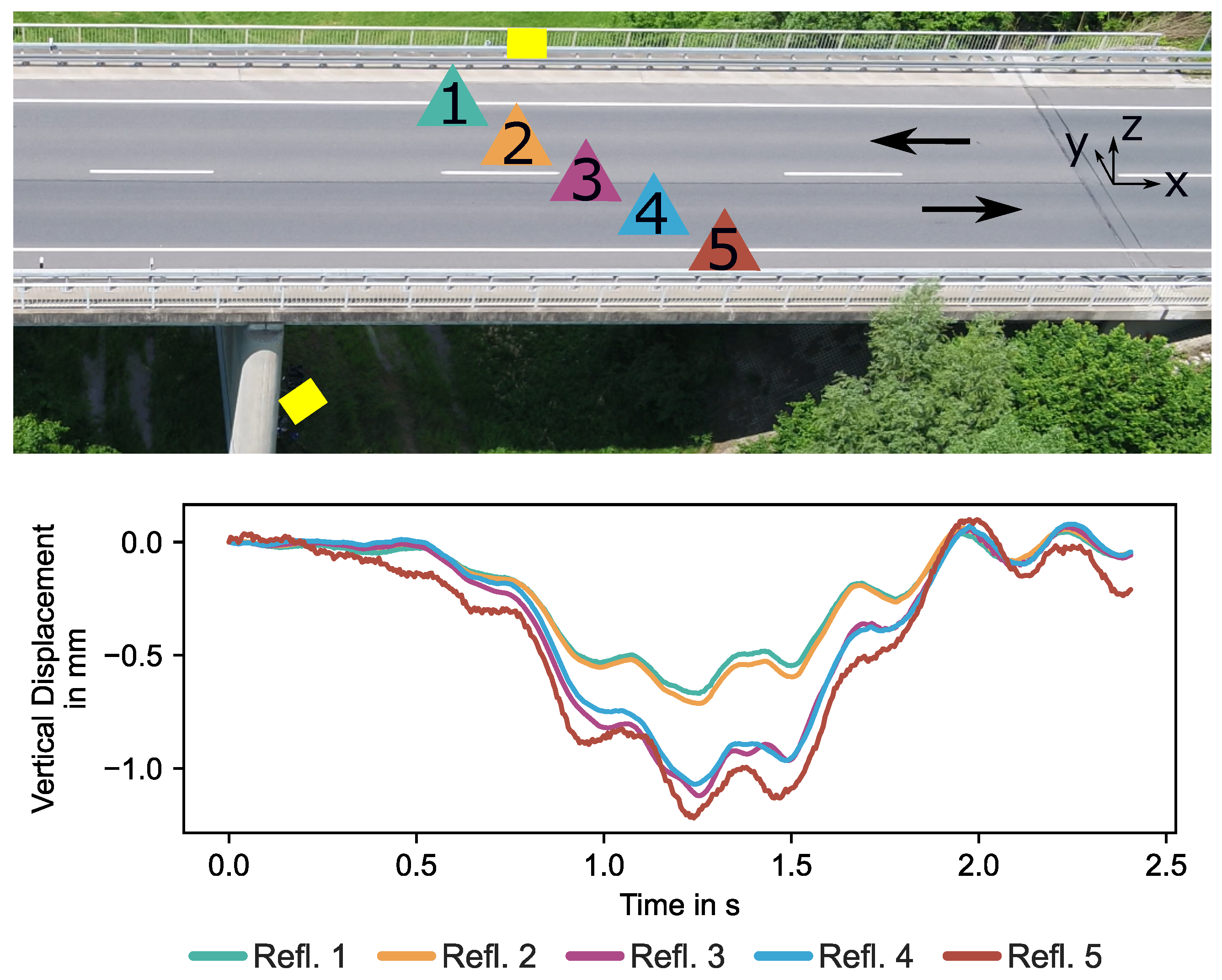
The offset of the reflectors in the y direction, as depicted in Figure 2, makes it possible to discern the vertical driving position of a vehicle. In the first step, the lane shall be determined in a classification task using reflectors 2 and 4. As a baseline, which we will refer to as POWER, we compare the signal power (Feature 9 in Table 3) for both reflectors. The lane is determined depending on which one has a higher value. The signal power of reflector 2 is greater, and the vehicle drives on lane 2. The input for the features-based models consists of the features 2, 3, and 9. In addition to the lane, the locus is estimated by regression to have a more precise vehicle localization. We use all 5 reflectors with the same features for locus regression.

4.5. Speed

Global responses, such as displacement, require a different approach than usual to calculate the speed since extracting it via peak detection from local responses is impossible. Therefore, we use data-driven ML to extract the vehicle speed. Arnold and Keller [10] and Arnold et al. [11] can extract vehicle crossings, but just using the length of such an event is not enough since the vehicle length also plays an important role. To show this, we additionally train a linear regression (LR) for speed estimation only on the signal length as a baseline. A one-dimensional LR tries to find the function of the coefficient w and the estimated intercept c, such that

$$y=w·x+c.$$

(8)

y is the target vector and x the input vector. In our case, x represents the event length, and y represents the vehicle speed. The feature-based models are trained with the features 1 to 11 from Table 3. As the input time series, we use reflector 3.

4.6. Axle Count

We treat the determination of the axle count as a classification problem with either 2, 3, 4, or 5+ axles. With more data, a more precise classification might be possible. All predictions are made using only the signal of reflector 3.

Unlike the previous task, we do not use the displacement directly as input or for feature extraction. Instead, we filter the signal with a 50th order forward-backward Butterworth high-pass with a cut-off frequency of 45 $\mathrm{Hz}$. This is performed so that the models learn high-frequency features and do not use low frequencies. For our feature-based approaches, we use the features from 1 to 10 in Table 3. We drop feature 11 since we already filter the signal with a high pass.

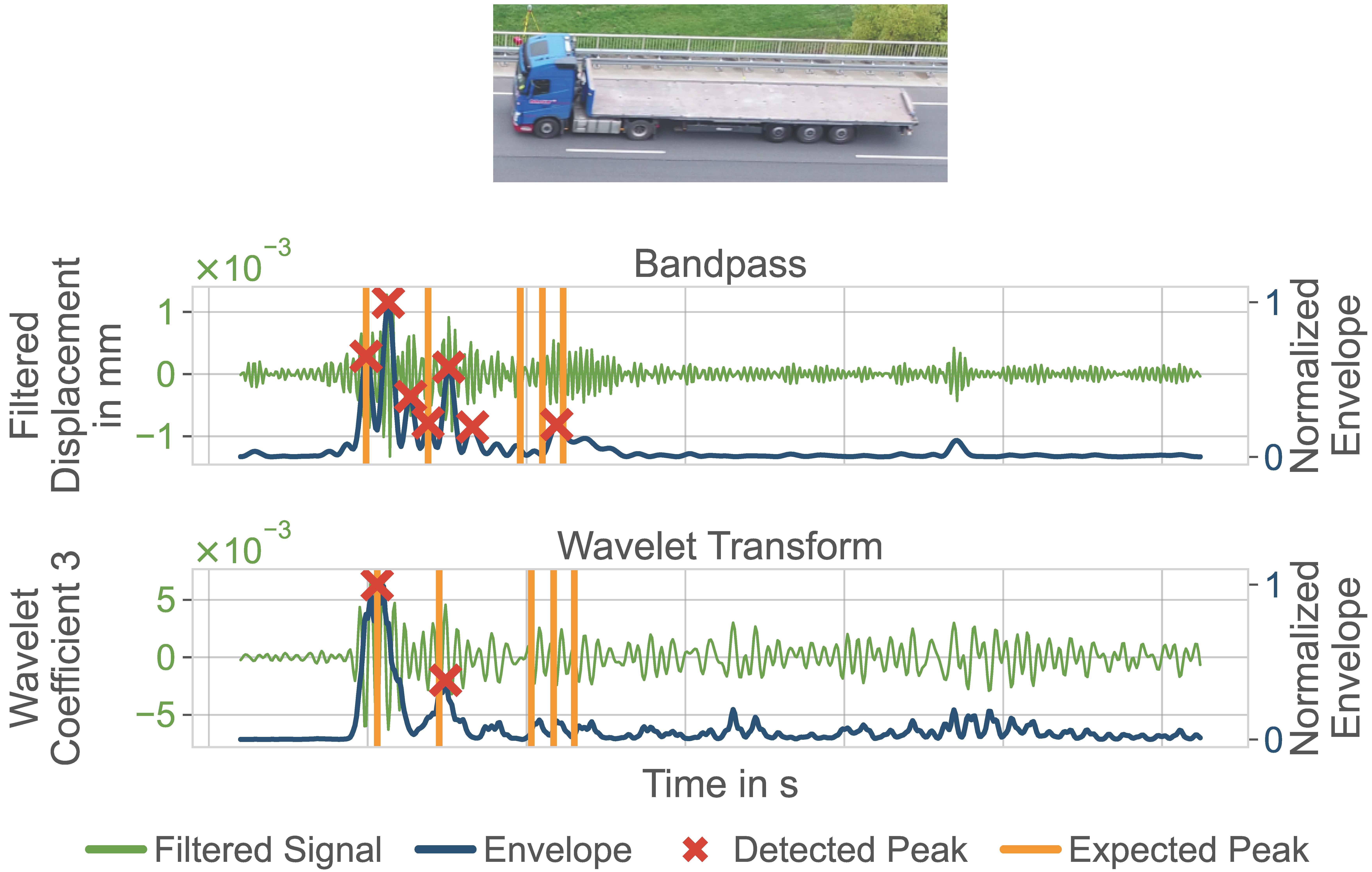
Apart from using ML, we also investigate the deterministic methods using a bandpass filter (BANDPASS) and CWT (WAVELET)  as novel approaches. Their pipelines are depicted in Figure 6 and Figure 7, respectively. They are similar except for the first step of the pipeline, where its corresponding filtering or transformation is applied. As input, they receive unfiltered GBR bridge displacement data from one reflector. The output consists of a list of the positions of the detected peak. For BANDPASS, we apply a forward-backward Butterworth bandpass in the first step. The order of the filter is 50 and the critical frequencies are (45 $\mathrm{Hz}$, 65 $\mathrm{Hz}$). We choose gaus7 as implemented by Lee et al. [31] and the $3.$ coefficient for our WAVELET approach. This corresponds to $m=7$ regarding Equation (6). These parameters have been determined as part of the parameter tuning process but outside the grid search. The bandpass-filtered signal and the wavelet transform result are then squared and smoothed by a weighted moving-average filter to obtain the distinguishable peaks. Ultimately, the signals are normalized to their highest value before searching all peaks to achieve generalization over all vehicles. We use the find_peaks-method of the Python-package scipy for peak detection [35]. The window size of the moving-average filter and the distance and prominence of a peak during peak detection are regarded as hyperparameters and deduced using the training dataset. Depending on the driving side and thus the driving direction, we discard peaks in half of the signal during which the vehicle does not enter or leave the bridge. 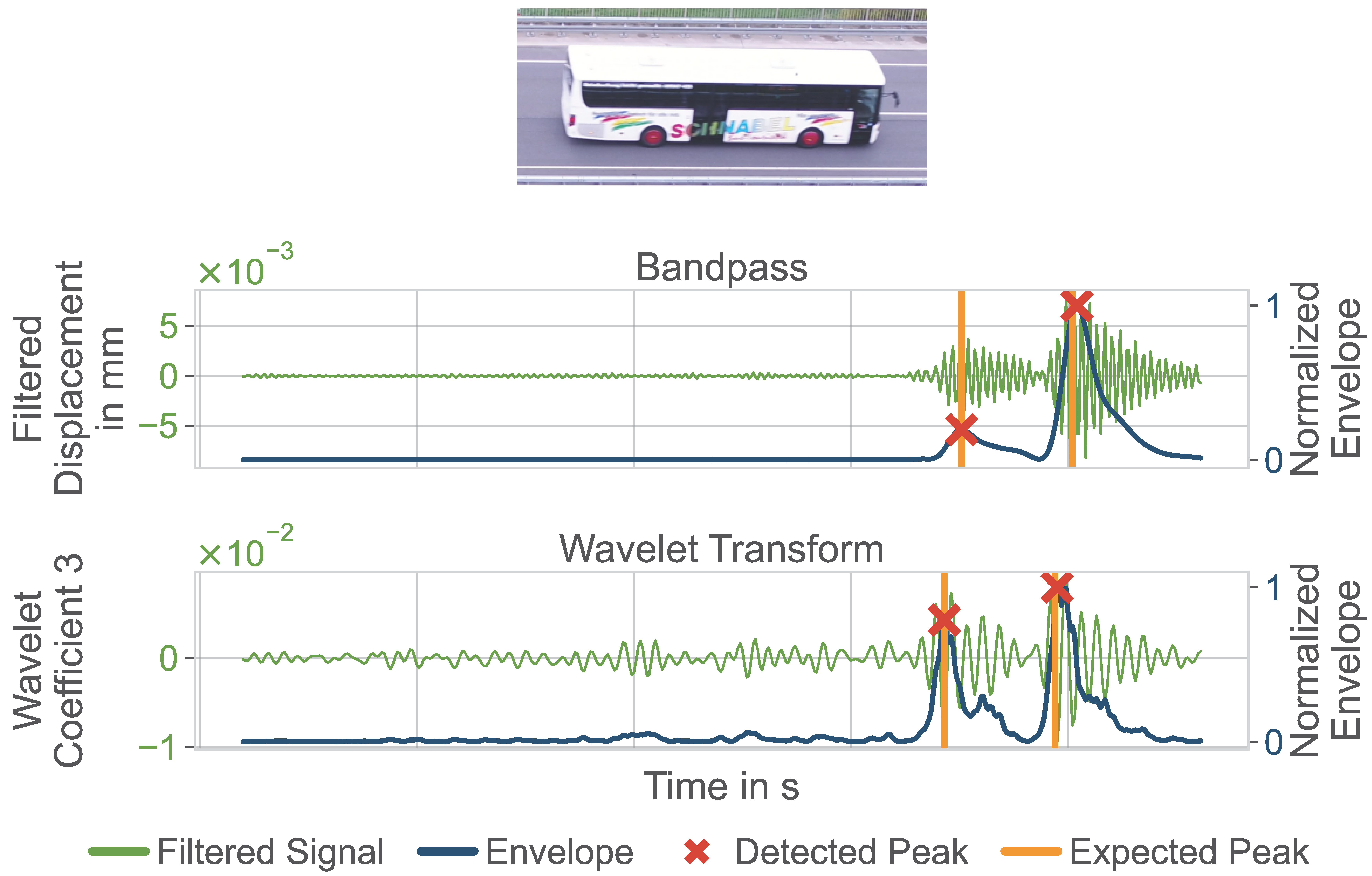As seen from Figure 8 andFigure 9, only the entering or leaving process is relevant for peak detection. Finally, we treat the length of the list of detected peak positions as the axle count. If no peak or only one is detected, we assume two axles.

4.7. Axle Spacing

Finally, we investigate how well the distance of axles can be determined. We treat this as a multi-output regression. Our BANDPASS and WAVELET procedures return a list of detected peak positions x (see Figure 6 and Figure 7). A peak at position i in the list is interpreted as axle number i. The temporal distance between the peaks i and j can be calculated by subtracting the consecutive positions $x_j$ and $x_i$ and then divided by the GBR sampling rate of 200 $\mathrm{Hz}$. With the speed $v_{UAV}$ from the UAV data, this can finally be transformed into axle spacing $d_{ij}$ between axle i and j according to

$$d_{ij}=\frac{x_j-x_i}{200\mathrm{Hz}}·v_{UAV}.$$

(9)

We assume the speed can be correctly extracted from Section 4.5. We also assume that the axle count is known and ignore additionally detected spacings during evaluation. The same goes for our ML approaches. We also use the same inputs as in Section 4.6.

5. Results

This study aims to investigate the potential of GBR for contactless NOR BWIM. In this section, we will state the results of our methods described in Section 4 in a corresponding order. Each approach except vehicle type classification is evaluated once for all vehicles and once for only trucks since they are more relevant for SHM. Classification tasks are evaluated based on balanced accuracy (BA), overall accuracy (OA), precision (P), and recall (RC). Regression performance is expressed by the coefficient of determination ($R^2$), mean squared error (MSE), and mean absolute error (MAE). The results of our filtering approaches will be addressed in detail in Section 5.4.

5.1. Vehicle Type

The results for the distinction between cars and trucks, which is relevant for SHM, are displayed in

Table 4. Classification results for vehicle type estimation with reflectors 2 and 4. The highlighted values represent the best results for each vehicle group.

Model	BA	OA	P	RC
	in%	in%	in%	in%
MiniRocket	98.1	99.2	100	96.1
RF	100	100	100	100
GB	100	100	100	100
KNN	100	100	100	100

. All feature-based models classify the vehicle type perfectly. Using the raw time series data, only MiniRocket misclassifies one truck as a car.

5.2. Land and Locus

We investigate both lane classification (see

Table 5. Classification results for lane estimation with reflectors 2 and 4. The highlighted values represent the best results for each vehicle group.

Model	All Vehicles				Trucks Only
	BA	OA	P	RC	BA	OA	P	RC
	in%	in%	in%	in%	in%	in%	in%	in%
POWER	92.7	92.4	87.1	98.2	96.9	96.3	91.7	100
MiniRocket	94.3	90.0	98.2	94.1	96.9	96.3	91.7	100
RF	83.2	83.1	79.7	85.4	89.2	88.9	83.3	90.1
GB	93.3	93.2	91.2	94.5	93.8	92.6	83.3	90.1
KNN	93.4	93.2	89.8	96.4	92.3	92.6	90.1	90.1

) as well as locus regression (see

Table 6. Regression results for locus estimation with all five reflectors. The highlighted figures represent the best results for each vehicle group.

Model	All Vehicles			Trucks Only
	${\mathit{R}}^{\mathbf{2}}$	MSE	MAE	${\mathit{R}}^{\mathbf{2}}$	MSE	MAE
		in ${\mathit{m}}^{\mathbf{2}}$	in $\mathit{m}$		in ${\mathit{m}}^{\mathbf{2}}$	in $\mathit{m}$
LR	0.57	1.50	1.06	0.91	0.38	0.47
MiniRocket	0.84	0.57	0.54	0.96	0.18	0.36
RF	0.59	1.40	0.79	0.32	2.86	0.99
GB	0.80	0.69	0.57	0.91	0.40	0.49
KNN	0.81	0.65	0.50	0.99	0.04	0.16

), which is the lateral position of a vehicle. MiniRocket provides the best results for both vehicle groups with 94.3% and 97.9%. Except for RF, all models have a BA of over 90%. POWER shares the first place with MiniRocket in the case of only trucks. Both approaches misclassify only one truck, leading to an RC of 100%. Yet, RF, whose concept relies on comparing input values, has the worst results for both cases. The difference between both vehicle selections is slight, but the performance for only trucks is better overall.

A more fine granular lateral position estimation via the locus using all five reflectors resulted in Table 6. Again, MiniRocket beats all other models for all vehicles, with an $R^2$ of 0.84. When discarding cars, KNN has an almost perfect $R^2$ score of $0.99$, slightly surpassing the MiniRocket with 0.96. All models improve from all vehicles to only trucks, like in lane classification, except for RF, which achieves worse results.

5.3. Speed

Table 7. Regression results for speed estimation with reflector 3. The highlighted values represent the best MAE for each vehicle group.

Model	All Vehicles			Trucks Only
	${\mathit{R}}^{\mathbf{2}}$	MSE	MAE	${\mathit{R}}^{\mathbf{2}}$	MSE	MAE
		in ${\mathit{m}}^{\mathbf{2}}/{\mathit{s}}^{\mathbf{2}}$	in $\mathit{m}/\mathit{s}$		in ${\mathit{m}}^{\mathbf{2}}/{\mathit{s}}^{\mathbf{2}}$	in $\mathit{m}/\mathit{s}$
LR	0.71	5.08	1.81	0.67	2.22	1.22
MiniRocket	0.94	1.06	0.76	0.71	1.93	1.02
RF	0.85	2.68	1.12	0.53	3.16	1.25
GB	0.85	2.56	1.14	0.75	1.67	1.06
KNN	0.85	2.60	1.14	0.70	2.03	1.13

shows the results for the speed regression task. MiniRocket achieves the best performance for both vehicle sets. For all vehicles, it achieves an $R^2$ of 0.94 and an MAE of $0.76$ $\mathrm{m}$/$\mathrm{s}$, which is slightly better than the $0.86$ $\mathrm{m}$/$\mathrm{s}$ of Kawakatsu et al. [23]. All feature-based methods have comparable results for $R^2$ and are less effective than MiniRocket. LR, on only the duration of the bridge crossing event, has the worst results but still is not far off from MAE. Its MSE, however, is significantly worse compared to the other models.

LR does improve regarding MSE and MAE when only using trucks, although $R^2$ decreases. The same behavior can be observed for KNN and GB. GB has the best $R^2$ for trucks and is slightly worse than MiniRocket in MSE and MAE. MiniRocket, with an MAE of $1.02$ $\mathrm{m}$/$\mathrm{s}$ is still only $0.16$ $\mathrm{m}$/$\mathrm{s}$ worse than Kawakatsu et al. [23]. However, they evaluate more data, making their results more robust.

5.4. Axle Count

As explained in Section 4.6, we investigate the potential of bandpass filtering and wavelet transform to detect axles in GBR bridge displacement data. Three examples of these approaches can be seen in Figure 8, Figure 9 and Figure 10. In all images, first, the vehicle is depicted, and then the results of the filtering and the smoothed time series. The filtered signal corresponds to the intermediate result after the bandpass filtering and CWT in Figure 6 and Figure 7, respectively. The envelope represents the unitless waveform after the normalization step from which the peak positions are acquired. We have marked the peaks, which have been detected with the respective approach and the learned hyperparameters. Finally, starting from the first detected peak, positions where we would expect subsequent peaks due to the labeled UAV data are shown.

Figure 8 shows the bus with two axles from Figure 3. The bandpass filtered signal has two areas with a high amplitude vibration in the frequency range of 45 $\mathrm{Hz}$ to 65 $\mathrm{Hz}$. Accordingly, the envelopes for both approaches have two peaks. Assuming that the first peak corresponds to the first axle, the second peak matches the expected position. A more complex example is depicted in Figure 9 since the truck has five axles, three of which are very close to each other. Again, these axles are recognizable and at their expected position in the bandpass signal and its envelope. However, one additional peak does not belong to any axle. This peak does not exist in the wavelet signal. Conversely, the first peak is missed, and the final three axles are combined into one axle group in the signal. Finally, Figure 10 shows a truck with a similar axle configuration. Seven peaks are detected using the BANDPASS approach. The final three axles are again registered as a single axle group. WAVELET clearly shows the first two axles at the expected positions, yet the peaks for the three back axles are too small to be distinguishable from noise. The behavior in the previous pictures is also evident with cars, although they are usually lighter.

We also investigated the other reflectors as well as the second GBR. While very distinct peaks, like in Figure 8, are also visible with other reflectors, reflector 3 shows the best results overall. No axle information could be extracted from the second GBR using our two methods, BANDPASS and WAVELET.

As described in Section 4.6, the hyperparameters for BANDPASS and WAVELET have been determined using the training data. To quantify the performance,

Table 8. Classification results for axle count estimation with reflector 3. The highlighted figures represent the best results for each vehicle group.

Model	All Vehicles				Trucks Only
	BA	OA	P	RC	BA	OA	P	RC
	in%	in%	in%	in%	in%	in%	in%	in%
BANDPASS	23.4	34.7	24.5	23.4	35.1	29.6	30.3	35.2
WAVELET	25.1	28.8	21.5	25.0	46.6	37.0	44.6	46.6
MiniRocket	60.7	86.4	58.1	60.7	76.7	70.4	74.4	76.7
RF	50.5	89.0	46.0	50.5	45.4	51.9	23.7	45.5
GB	40.8	83.9	38.0	40.9	38.6	48.1	32.0	38.6
KNN	47.0	87.3	46.0	47.0	45.3	51.8	40.9	45.3

displays the results for all approaches. Again, MiniRocket has the best results for both categories. Especially for trucks, it achieves a BA of 76.7%, delivering results comparable to Kawakatsu et al. [21], who achieve BA of 85.8% using a single strain sensor. When including the cars, however, the BA decreases to only 60.7%. Only the OA improves compared to the trucks. BANDPASS and WAVELET have similar results for all vehicles, with WAVELET having a slightly better BA. Still, the BA is only 25.1%. It improves together with P and RC to 46.6% for only trucks, whereas BANDPASS achieves results of over 30%. RF, GB, and KNN tend to outperform BANDPASS and WAVELET but still fall heavily behind MiniRocket.

5.5. Axle Spacing

As shown in the previous section, it is challenging to formalize a procedure for BANDPASS and WAVELET, which works for all vehicles. The same goes for axle spacing since it builds upon the peak detection. Yet, we want to indicate that the information can sometimes be extracted successfully. A more generalized analysis will be performed afterward.

In Figure 8, two peaks are easily recognizable. Using their distance, the GBR sampling frequency of 200 $\mathrm{Hz}$, and the vehicle speed, we can calculate an axle spacing of $6.33$ $\mathrm{m}$ using Equation (9). Comparing this to the UAV axle spacing of $6.19$ $\mathrm{m}$, we overestimate the spacing by only $0.14$ $\mathrm{m}$. Likewise, the results for Figure 9 would deliver close values, as the expected peaks are near the detected positions. Yet, additional peaks, such as the third peak in Figure 9 for BANDPASS, would lead to underestimating the second axle spacing, as we would also overestimate the axle count by one. These challenges are reflected in the overall results in

Table 9. Regression results for axle spacing estimation with reflector 3. The highlighted figures represent the best results for each vehicle group.

Model	All Vehicles			Trucks Only
	${\mathit{R}}^{\mathbf{2}}$	MSE	MAE	${\mathit{R}}^{\mathbf{2}}$	MSE	MAE
		in ${\mathit{m}}^{\mathbf{2}}$	in $\mathit{m}$		in ${\mathit{m}}^{\mathbf{2}}$	in $\mathit{m}$
BANDPASS	−0.22	3.80	0.54	−0.45	7.78	1.30
WAVELET	−0.14	3.54	0.49	−0.16	6.25	1.19
MiniRocket	0.45	1.71	0.27	0.66	1.78	0.64
RF	0.53	1.45	0.23	0.63	2.00	0.71
GB	0.53	1.45	0.21	0.68	1.73	0.66
KNN	0.43	1.75	0.22	0.64	1.95	0.68

. The $R^2$ is even harmful for both BANDPASS and WAVELET. While the MAE is only slightly more than 1 $\mathrm{m}$ for only trucks, the MSE shows that there are a lot of spacings estimated with large deviations, as previously outlined. The same tendency can be found when including cars. Interestingly, all ML approaches achieve similar results. MiniRocket has the best results for MAE with $0.64$ $\mathrm{m}$ for only trucks. Also, the MSE is considerably smaller for the ML approaches, meaning fewer outliers exist. With all vehicles, GB achieves the best MAE of $0.21$ $\mathrm{m}$, although all models achieve similar results again.

6. Discussion

The central focus of this study is the potential of GBR displacement signals for a remote and data-driven BWIM. This section will discuss the results stated in the previous section. First, we will analyze the potential of ML for all classification and regression tasks. Afterward, our filter approaches regarding axle configuration identification are discussed.

6.1. Machine Learning for Displacement-Based BWIM

As the results for vehicle-type classification are immaculate for feature-based methods, it is possible only to regard trucks for SHM if desired. Trucks cause a significantly greater deflection than cars. Therefore, the promising results are unsurprising. The issue of the driving lane can be avoided by using one reflector per lane as input data. Our distinction between vehicle types during vehicle configuration tasks is thus well founded.

It seems that, for all tasks except axle spacing estimation, ML models can extract vehicle configurations. MiniRocket, which uses the raw time series data and extracts features via convolutional kernels, shows especially auspicious results. The model with the best performance can vary from task to task, but MiniRocket either has the best performance or follows close behind. Interpretability is an important aspect of bridge monitoring [36,37,38]. The overall satisfying results of our models indicate that the extracted configurations are identifiable from global bridge displacement data using data-driven ML approaches.

To acquire the vertical position of a vehicle, we test both a lane classification and a locus regression. The lane can successfully be extracted for both vehicle categories. Trucks can be classified almost perfectly, with only one vehicle misclassified. This is unsurprising, as our reflectors are spread along the y axis (see Figure 2). Accordingly, the maximum displacement during an event correlates to the driving side. Especially for heavy vehicles, a clear distinction can be made. In Figure 2, e.g., reflectors 3 to 5 show a steeper curve than reflector 1 and 2. This suggests that the vehicle drives in lane 1, which corresponds to the bus from Figure 8, which caused the bending. Thus, it seems enough for trucks to compare the signal power of reflectors 2 and 4 to acquire the lane.

The locus regression shows a similar behavior in that the results improve when discarding cars. Due to KNN’s outstanding performance, we surmise that scaling our features will help with this task. This makes sense, as the maxima ratio within one event is more relevant than their absolute values.

There is a significant difference in speed between all vehicles and only trucks. The reason for this might lie in the dataset composition. As cars are more frequent and with less variation in the vehicle configurations, like the length, the correlation between event duration and speed is more prominent. Thus, for some models, the $R^2$ decreases while the MAE improves. For MiniRocket, $R^2$ and MAE decrease when discarding cars, suggesting that it does not mainly look at the event duration.

The results for axle count classification imply that our features from Table 3 are not helpful for this task, as all models that depend upon them have a BA of less than 51%. Only MiniRocket achieves satisfactory results, especially for trucks. The high OA but low BA show that the imbalance in the dataset, when including cars, leads to more misclassified trucks.

Comparing both datasets, it can be said that, although having more data generally helps, cars drastically change the distribution of many configurations. This makes it more challenging for models to learn truck properties. Regarding BWIM, where only trucks are considered relevant, this can be seen as a disadvantage. The truck dataset is very small as we have only one truck with seven axles, for example. Since trucks come in significant axle count and spacing variations, our models naturally have generalized difficulties. The dilemma of high imbalance and a small dataset is also apparent for axle spacing regression. Here, the MSE is very high for all vehicles compared to MAE, as the axle spacing for cars is very closely distributed (see Figure 4). Conversely, models mainly learn about the car distribution, regarding trucks as outliers due to the highly imbalanced datapoints.

6.2. Filtering for Axle Configuration Identification

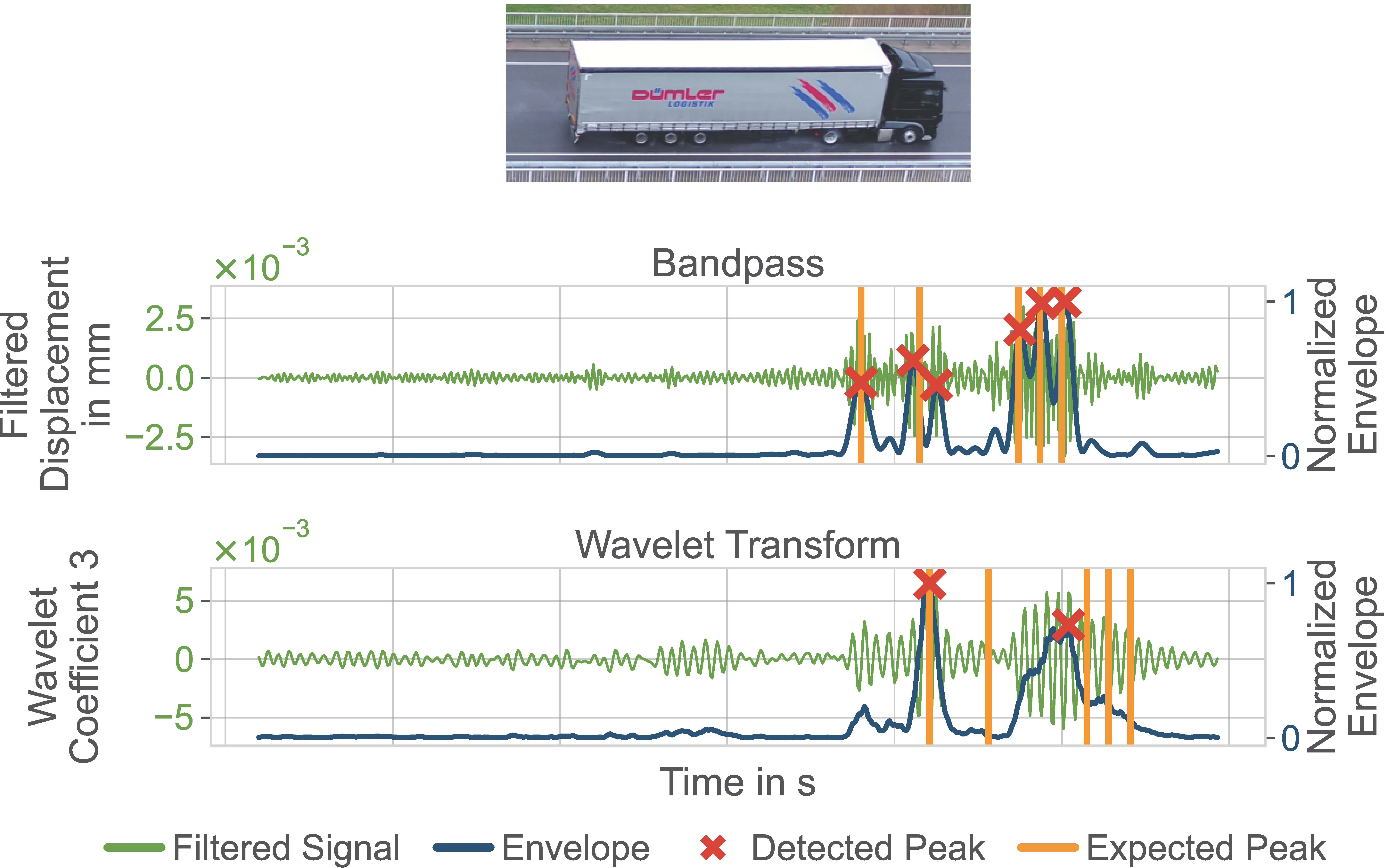
Figure 8, Figure 9 and Figure 10 indicate that the information of axles is present in a bridge’s global displacement time series. Individual examples produce promising results concerning axle count and axle spacing. To our knowledge, this has not been presented before, as displacement is barely exploited in BWIM. However, the results for BANDPASS and WAVELET in Table 8 and Table 9 show that it is challenging to find a general procedure. Especially the negative $R^2$ values in Table 9 demonstrate this, as this means that simply using the mean of the data as a prediction is a better fit than our methods. Neither BANDPASS nor WAVELET can be described as the better approach overall, as their respective performances varied heavily between samples. Unfortunately, we can only show a small portion of all the recorded vehicles, as there are cases in which no axle-induced peaks are visible in the bandpass signal, but they exist with WAVELET.

While having a high SNR to measure these small vibrations is necessary, a good SNR alone will not lead to valuable measurements concerning axle detection. Interestingly enough, the weight of a vehicle or axle seems not to be the decisive factor, as for some cars, the peaks are easily recognizable, whereas they are not visible for trucks. Therefore, we assume that the relative axle weight within one event is relevant. The truck in Figure 10 appears heavier in the front than in the back. Accordingly, the peaks for the latter axles are less visible. However, this is only a conjecture since no axle load data have been recorded during this study. Also, the driving direction appears unrelated to how well axles can be detected. More peaks might have been detected with a higher sampling frequency, or at least their distinction might have been more straightforward for CWT. Yu et al. [24] have demonstrated that a sampling frequency of only 200 $\mathrm{Hz}$ leads to large errors. These vibrations seem to be caused at the junction between the bridge and the street. Consequently, this behavior might be specific to this bridge. Since we only monitored one field, we cannot say if the same vibrations can be measured for the other junction. Both fields seem too loosely coupled to transmit the signal if they exist. For one-span bridges, both leaving and entering might be observable. In such cases, our BANDPASS and WAVELET approaches can also extract the vehicle speed. In this study, however, this was not possible.

For vehicles with clearly visible peaks, like in Figure 8, the axle-induced response could also be observed in the signal of other reflectors. This suggests that the specific reflector or its attachment does not induce the vibration but is a high-frequency vibration in the bridge displacement. Also, as mentioned in Section 3.1, we monitor the bridge with two GBRs that measure different components. There have not been visible vibrations or peaks for the GBR measuring the z and y components, although the SNR lies in an adequate range. This indicates that the vibration mainly occurs in the x-component. However, a more detailed investigation is necessary.

7. Conclusions and Outlook

In this study, we discuss a novel data-driven, displacement-based BWIM approach. The data were recorded at a two-span bridge in Germany using GBR and a UAV for ground-truth data. We investigate the potential of both classic signal processing and ML to extract the vehicle configurations from bridge-crossing events. These configurations include vehicle type, speed, lane, locus, axle count, and spacing. One challenge herein is that displacement is a non-local bridge response. Furthermore, our dataset is imbalanced and consists of variable-length time series. We evaluate all approaches on all vehicles and all trucks only.

As ML approaches, we test four different models, three of which depend on manually crafted features. The fourth model, MiniRocket, uses the raw time series data. Over all configurations, MiniRocket achieves the most auspicious results, comparable to other studies such as Kawakatsu et al. [21]. While speed, lane, and locus can be extracted, axle count classification is more challenging for all models. Only MiniRocket can classify a truck axle count with a BA of 76.7%. Finally, the results for axle spacing regression suffer from a small dataset. Therefore, more bridges should be monitored. However, more complex models and using extracted values like speed as an input feature could lead to better results.

We have recorded a high-frequency vibration for this bridge that coincides with axles crossing the junction. Using bandpass filtering and wavelet transform, we could demonstrate examples of this behavior. Based on this finding, we try two approaches for axle count and axle spacing determination purely based on signal processing. While the information seems available, we have not found a comprehensive procedure for the automatic extraction of axle configurations. A more sophisticated approach exploiting CNNs might be more successful as they can learn more generalizable features. For this, however, either the dataset needs to be increased, or data augmentation needs to be applied, as it has been investigated in Arnold and Keller [12]. Furthermore, it must be investigated whether other bridges show a similar behavior in the high-frequency range. Ideally, GBRs with a higher sampling rate will be used for these measurements.

We showed that a purely data-driven BWIM exploiting GBR-displacement time series data is possible. However, these promising results must be refined using a more extensive dataset. Ojio et al. [3] indicated that determining axle loads is possible with bridge displacement signals and the vehicle configurations extracted in this study. Thus, our results work towards a fully remote and data-driven BWIM.

References

1. Yu, Y.; Cai, C.; Deng, L. State-of-the-art review on bridge weigh-in-motion technology. Adv. Struct. Eng. 2016, 19, 1514–1530. [Google Scholar] [CrossRef]
2. Kawakatsu, T.; Aihara, K.; Takasu, A.; Adachi, J. Fully-Neural Approach to Heavy Vehicle Detection on Bridges Using a Single Strain Sensor. In Proceedings of the ICASSP 2020–2020 IEEE International Conference on Acoustics, Speech and Signal Processing (ICASSP), Barcelona, Spain, 4–8 May 2020; pp. 3047–3051, ISSN 2379-190X. [Google Scholar] [CrossRef]
3. Ojio, T.; Carey, C.H.; OBrien, E.J.; Doherty, C.; Taylor, S.E. Contactless Bridge Weigh-in-Motion. J. Bridge Eng. 2016, 21, 04016032. [Google Scholar] [CrossRef]
4. Gentile, C.; Bernardini, G. Output-only modal identification of a reinforced concrete bridge from radar-based measurements. NDT E Int. 2008, 41, 544–553. [Google Scholar] [CrossRef]
5. Michel, C.; Keller, S. Introducing a non-invasive monitoring approach for bridge infrastructure with ground-based interferometric radar. In Proceedings of the EUSAR 2021, 13th European Conference on Synthetic Aperture Radar, Online, 29 March–1 April 2021; pp. 1–5. [Google Scholar]
6. Michel, C.; Keller, S. Advancing Ground-Based Radar Processing for Bridge Infrastructure Monitoring. Sensors 2021, 21, 2172. [Google Scholar] [CrossRef]
7. Michel, C.; Keller, S. Determining and Investigating the Variability of Bridges’ Natural Frequencies with Ground-Based Radar. Appl. Sci. 2022, 12, 5354. [Google Scholar] [CrossRef]
8. Michel, C.E. Generic Radar Processing Methods for Monitoring Tasks on Bridge Infrastructure. Ph.D. Thesis, Karlsruher Institut für Technologie (KIT), Karlsruhe, Germany, 2023. [Google Scholar] [CrossRef]
9. Pieraccini, M.; Miccinesi, L.; Abdorazzagh Nejad, A.; Naderi Nejad Fard, A. Experimental Dynamic Impact Factor Assessment of Railway Bridges through a Radar Interferometer. Remote Sens. 2019, 11, 2207. [Google Scholar] [CrossRef]
10. Arnold, M.; Keller, S. Detection and classification of bridge crossing events with ground-based interferometric radar data and machine learning approaches. ISPRS Ann. Photogramm. Remote Sens. Spat. Inf. Sci. 2020, V-1-2020, 109–116. [Google Scholar] [CrossRef]
11. Arnold, M.; Hoyer, M.; Keller, S. Convolutional neural networks for detecting bridge crossing events with ground-based interferometric radar data. ISPRS Ann. Photogramm. Remote Sens. Spat. Inf. Sci. 2021, V-1-2021, 31–38. [Google Scholar] [CrossRef]
12. Arnold, M.; Keller, S. Machine-learning for analyzing bridge displacement using radar data. In Proceedings of the Bridge Maintenance, Safety, Management, Life-Cycle Sustainability and Innovations; CRC Press: Boca Raton, FL, USA, 2024. [Google Scholar]
13. Zhao, X.; Liu, H.; Yu, Y.; Xu, X.; Hu, W.; Li, M.; Ou, J. Bridge Displacement Monitoring Method Based on Laser Projection-Sensing Technology. Sensors 2015, 15, 8444–8463. [Google Scholar] [CrossRef] [PubMed]
14. Dau, H.A.; Bagnall, A.; Kamgar, K.; Yeh, C.C.M.; Zhu, Y.; Gharghabi, S.; Ratanamahatana, C.A.; Keogh, E. The UCR Time Series Archive. arXiv 2019, arXiv:1810.07758. [Google Scholar] [CrossRef]
15. Bier, A.; Jastrzebska, A.; Olszewski, P. Variable-Length Multivariate Time Series Classification Using ROCKET: A Case Study of Incident Detection. IEEE Access 2022, 10, 95701–95715. [Google Scholar] [CrossRef]
16. Ruiz, A.P.; Flynn, M.; Large, J.; Middlehurst, M.; Bagnall, A. The great multivariate time series classification bake off: A review and experimental evaluation of recent algorithmic advances. Data Min. Knowl. Discov. 2021, 35, 401–449. [Google Scholar] [CrossRef] [PubMed]
17. Dempster, A. ROCKET: Exceptionally fast and accurate time series classification using random convolutional kernels. Data Min. Knowl. Discov. 2020, 34, 1454–1495. [Google Scholar] [CrossRef]
18. Dempster, A.; Schmidt, D.F.; Webb, G.I. MINIROCKET: A Very Fast (Almost) Deterministic Transform for Time Series Classification. arXiv 2021, arXiv:2012.08791. [Google Scholar] [CrossRef]
19. Löning, M.; Bagnall, A.; Ganesh, S.; Kazakov, V. Sktime: A Unified Interface for Machine Learning with Time Series. arXiv 2019, arXiv:1909.07872. [Google Scholar]
20. Hertel, L.; Phan, H.; Mertins, A. Classifying Variable-Length Audio Files with All-Convolutional Networks and Masked Global Pooling. arXiv 2016, arXiv:1607.02857. [Google Scholar]
21. Kawakatsu, T.; Aihara, K.; Takasu, A.; Adachi, J. Deep Sensing Approach to Single-Sensor Bridge Weighing in Motion. In Proceedings of the 9th European Workshop on Structural Health Monitoring, Manchester, UK, 10–13 July 2018. [Google Scholar]
22. Kawakatsu, T.; Aihara, K.; Takasu, A.; Adachi, J. Deep Sensing Approach to Single-Sensor Vehicle Weighing System on Bridges. IEEE Sens. J. 2019, 19, 243–256. [Google Scholar] [CrossRef]
23. Kawakatsu, T.; Aihara, K.; Takasu, A.; Nagayama, T.; Adachi, J. Data-Driven Bridge Weigh-In-Motion. IEEE Sens. J. 2023, 23, 17064–17077. [Google Scholar] [CrossRef]
24. Yu, Y.; Cai, C.; Deng, L. Vehicle axle identification using wavelet analysis of bridge global responses. J. Vib. Control 2017, 23, 2830–2840. [Google Scholar] [CrossRef]
25. Lechner, B.; Lieschnegg, M.; Mariani, O.; Pircher, M.; Fuchs, A. A Wavelet-Based Bridge Weigh-In-Motion System. Int. J. Smart Sens. Intell. Syst. 2010, 3, 573–591. [Google Scholar] [CrossRef]
26. Zhao, H.; Tan, C.; OBrien, E.J.; Uddin, N.; Zhang, B. Wavelet-Based Optimum Identification of Vehicle Axles Using Bridge Measurements. Appl. Sci. 2020, 10, 7485. [Google Scholar] [CrossRef]
27. Gentile, C.; Bernardini, G. An interferometric radar for non-contact measurement of deflections on civil engineering structures: Laboratory and full-scale tests. Struct. Infrastruct. Eng. 2010, 6, 521–534. [Google Scholar] [CrossRef]
28. Tzuta, L. LabelImg. 2015. Available online: https://github.com/tzutalin/labelImg (accessed on 17 July 2023).
29. Kaiser, G. A Friendly Guide to Wavelets; Birkhäuser: Boston, MA, USA, 2011. [Google Scholar] [CrossRef]
30. Rosyidi, S.A.P.; Taha, M.R.; Chik, Z.; Ismail, A. Signal reconstruction of surface waves on SASW measurement using Gaussian Derivative wavelet transform. Acta Geophys. 2009, 57, 616–635. [Google Scholar] [CrossRef]
31. Lee, G.R.; Gommers, R.; Waselewski, F.; Wohlfahrt, K.; O’Leary, A. PyWavelets: A Python package for wavelet analysis. J. Open Source Softw. 2019, 4, 1237. [Google Scholar] [CrossRef]
32. Breiman, L. Random Forests. Mach. Learn. 2001, 45, 5–32. [Google Scholar] [CrossRef]
33. Friedman, J.H. Greedy Function Approximation: A Gradient Boosting Machine. Ann. Stat. 2001, 29, 1189–1232. [Google Scholar] [CrossRef]
34. Cover, T.; Hart, P. Nearest neighbor pattern classification. IEEE Trans. Inf. Theory 1967, 13, 21–27. [Google Scholar] [CrossRef]
35. Virtanen, P.; Gommers, R.; Oliphant, T.E.; Haberland, M.; Reddy, T.; Cournapeau, D.; Burovski, E.; Peterson, P.; Weckesser, W.; Bright, J.; et al. SciPy 1.0: Fundamental Algorithms for Scientific Computing in Python. Nat. Methods 2020, 17, 261–272. [Google Scholar] [CrossRef]
36. Kuok, S.C.; Yuen, K.V. Investigation of modal identification and modal identifiability of a cable-stayed bridge with Bayesian framework. Smart Struct. Syst. 2016, 17, 445–470. [Google Scholar] [CrossRef]
37. Kim, S.; Kim, N.; Park, Y.S.; Jin, S.S. A Sequential Framework for Improving Identifiability of FE Model Updating Using Static and Dynamic Data. Sensors 2019, 19, 5099. [Google Scholar] [CrossRef] [PubMed]
38. Katafygiotis, L.S.; Lam, H.F.; Papadimitriou , C. Treatment of Unidentifiability in Structural Model Updating. Sensors 2000, 3, 19–39. [Google Scholar]
Figure 1. Measurement setup applied in this study. The GBR measures the bridge displacement from underneath it. The UAV records the bridge deck with a camera for traffic ground-truth data.
Infrastructures 09 00037 g001
Figure 2. Overview of the bridge and an example displacement time series. The yellow rectangles in the upper image represent the GBRs, and the numbered triangles represent the five reflectors at their approximate position.
Infrastructures 09 00037 g002
Figure 3. Example of a labeled vehicle using the tool provided by Tzuta [28]. Bounding boxes have been drawn around the axles, as indicated by the orange bounding boxes. The yellow circles represent two control points for the coordination transformation. Furthermore, the lane number is shown.
Infrastructures 09 00037 g003
Figure 4. Distributions of speed, locus, and axle spacing in the applied dataset.
Infrastructures 09 00037 g004
Figure 5. Methodology for our feature-based methods. F 1 F N represent manually extracted features. We use a high-pass filter before feature extraction for the axle counting and axle spacing estimation.
Infrastructures 09 00037 g005
Figure 6. Pipeline for our BANDPASS approach for axle configuration extraction. The orange-colored hyperparameters are determined during the grid search. The lane information is used in the Discard Peaks step as an additional input parameter to filter the detected peaks.
Infrastructures 09 00037 g006
Figure 7. Pipeline for our WAVELET approach for axle configuration extraction. The orange-colored hyperparameters are determined during the grid search. The lane information is used in the Discard Peaks step as an additional input parameter to filter the detected peaks.
Infrastructures 09 00037 g007
Figure 8. Example result of a bus for our filtering approaches.
Infrastructures 09 00037 g008
Figure 9. Example result of a truck for our filtering approaches.
Infrastructures 09 00037 g009
Figure 10. Second example result of a truck for our filtering approaches.
Infrastructures 09 00037 g010