Analysis of Road Infrastructure and Traffic Factors Influencing Crash Frequency: Insights from Generalised Poisson Models ^†

Abstract

This research utilises statistical modelling to explore the impact of roadway infrastructure elements, primarily those related to cross-section design, on crash occurrences in urban areas. Cross-section design is an important step in the roadway geometric design process as it influences key operational characteristics like capacity, cost, safety, and overall functionality of the transport system entity. Evaluating the influence of cross-section design on these factors is relatively straightforward, except for its impact on safety, especially in urban areas. The safety aspect has resulted in inconsistent findings in the existing literature, indicating a need for further investigation. Negative binomial (NB) models are typically employed for such investigations, given their ability to account for over-dispersion in crash data. However, the low sample mean and under-dispersion occasionally exhibited by crash data can restrict their applicability. The generalised Poisson (GP) models have been proposed as a potential alternative to NB models. This research applies GP models for developing crash prediction models for urban road segments. Simultaneously, NB models are also developed to enable a comparative assessment between the two modelling frameworks. A six-year dataset encompassing crash counts, traffic volume, and cross-section design data reveals a significant association between crash frequency and infrastructure design variables. Specifically, lane width, number of lanes, road separation, on-street parking, and posted speed limit are significant predictors of crash frequencies. Comparative analysis with NB models shows that GP models outperform in cases of low sample mean crash types and yield similar results for others. Overall, this study provides valuable insights into the relationship between road infrastructure design and crash frequency in urban environments and offers a statistical approach for predicting crash frequency that maintains a balance between interpretability and predictive power, making it more viable for practitioners and road authorities to apply in real-world road safety scenarios.

1. Introduction

Road crashes are undesirable outcomes of transportation activities, resulting in fatalities, injuries, property damages, financial losses, and time delays on the one hand, called direct costs; they also have repercussions like missed workdays, energy waste, and economic and psychological consequences on the other hand, called indirect costs [1]. To mitigate these costs, several countries have set ambitious goals of eliminating all fatal and severe injury crashes from their roads by adopting systematic approaches towards traffic safety through initiatives like ‘vision zero’ and ‘safe system approach’ [2,3]. With a thorough understanding of the underlying causes of vehicle crashes and the implementation of suitable countermeasures, this goal is indeed achievable.

Transportation researchers utilise various techniques to understand the crash phenomenon, such as crash investigation reports, video analysis, naturalistic driving studies, simulation studies, crash data statistical analysis, artificial neural networks, surrogate safety measures, and telematics data analysis [4,5,6,7]. Safety performance functions (SPFs)—statistical models for crash prediction—have been the subject of many studies during the past few decades [8,9,10,11]. The SPFs, alternatively called crash prediction models, are regression models that quantitatively capture the association between traffic and roadway system attributes, including infrastructure elements and crash frequency on a specific transportation facility (e.g., road segment, intersection, interchange, etc.). They are used in crash hotspot identification, treatment effectiveness evaluation, alternate countermeasure comparison, and roadway safety improvement programs incorporating safety-related considerations into their design and standards [12,13,14]. Highway Safety Manual (HSM), a publication by the American Association of State Highway and Transportation Officials (AASHTO), provides probably the most comprehensive collection of the SPFs for various facility types, site types, crash types, and crash severity levels [15]. Given that the HSM SPFs are developed using the data from only a few states in the US, the direct application of these SPFs in other jurisdictions requires calibration to account for differences in traffic conditions, local laws, road infrastructure, and people’s behaviour. Consequently, many studies have calibrated SPFs to assure their applicability in different regions [16,17,18]. The HSM also recommends the estimation of new SPFs in jurisdictions where sufficient data are available. This has led to the estimation of SPFs in other regions using local datasets; for example, see [19,20,21].

Analysts develop distinct SPFs for urban and rural roadways due to the (potential) differences in crash predictors in these environments [10,11]. Typical urban area characteristics, such as high-density development, aggressive land-use planning, local regulations, on-street parking, bike lanes, and mixed traffic, generally make traffic safety problems, solutions, and analysis more complex [22]. Despite that, numerous studies have developed models for urban roads, exploring the effects of traffic and roadway infrastructure attributes, including average annual daily traffic (AADT), number of lanes, lane width, on-street parking, speed limits, etc., on crash occurrence [23,24,25,26]. For example, Liu et al. [23] estimated crash prediction models (SPFs and crash prediction models are used interchangeably in this text) for urban segments and reported that AADT per lane, the number of lanes, and segment length had significant non-positive effects on crashes and that segments with lower speed limits were associated with more crashes than those with higher speed limited (45 mph (70 km/h) or above). Kim et al. [11] developed crash prediction models for single and multi-vehicle crashes on urban and suburban arterials using simple annual average daily traffic (AADT) and log-transformed AADT. The authors found that the simple AADT models outperformed the log-transformed AADT models. Vieira Gomes [20] reported developing and applying SPFs for several highway safety analyses after discovering that the calibrated models from other regions were inadequate for local urban conditions in Lisbon [27]. In urban areas, roadway cross-section design has a somewhat complicated relationship with the occurrence of crashes, as indicated by varying results in the literature [25]. For example, Potts et al. [28] noticed no increase in crash frequency on urban and suburban road segments and intersection approaches with lanes narrower than 12 ft (3.6 m). Rista et al. [29] developed models to study the impact of lane width on the sideswipe-same direction and rear-end crashes for four functional classes of urban roads. The authors reported that wider lanes were related to fewer crashes than narrower lanes, indicating increased safety performance. Park and Abdel-Aty [24] studied the effects of multiple roadway cross-section elements (e.g., road lane, bike lane, median, and shoulder widths) on crash occurrence on urban arterials for various crash types and severity levels. Their results indicated a significant increase in safety performance with an increase in the width of the median and the shoulder. However, the changes in safety performance were non-linear for increases in the width of roadway lanes and bike lanes. Sharma et al. [30] studied the safety and operational effects of lane width of midblock segments and signalised intersection approaches in urban areas by developing random-parameter Poisson and NB models. The authors found an increase in safety with an increase in the lane width from 10 ft to 11 ft and 12 ft when the speed limit was lower (35 m/h = 55 km/h). For higher speed areas, this relationship was not very clear.

Methodologically, researchers have recently utilised relatively advanced statistical models for crash data analysis and developing SPFs [29,31,32,33]. Nevertheless, consensus on applying the conventional NB model for developing crash prediction models remains unmatched across the transportation safety community, partly because of its ability to accommodate over-dispersion and partly because of the ease associated with its estimation procedure and interpretation. Despite its advantages, the NB models suffer limitations in fitting the under-dispersion observed in crash data on certain occasions [34]. Theoretically speaking, the NB model could be adjusted to handle the under-dispersion by setting the shape parameter as negative, i.e., (Var (Y) = μ + (−α) μ²). However, this adjustment would make the conditional mean of the Poisson no longer gamma distributed and lead to misspecification of its probability density function [35], underestimated standard errors [36], and thus unreliable parameter estimates [37].

Moreover, crash data are occasionally characterised by a low sample mean problem [38,39], for instance, when a limited number of observations are recorded for a specific crash type on a given network [39]. The low sample mean results in biased estimates of regression coefficients and negatively affects regression models [38]. Conventional NB models cannot effectively handle datasets with low sample means because the gamma-distributed error terms related to the mean of the Poisson distributed variables in the NB models are restrictive in accounting for heterogeneity across observations [40]. As a solution, some studies have explored alternative regression models (e.g., Poisson–lognormal, the negative binomial (NB) bootstrap maximum likelihood estimation (MLE) method, and the NB-Lindley model) to deal with these problems [32,33]. Others proposed the application of zero-inflated variants of the count models, especially when the percentage of zero observations in crash data is substantially large; e.g., see [41]. However, the application of zero-inflated models to model vehicle crashes has been shown to be inappropriate mainly due to theoretical inconsistencies; e.g., [42]. In this situation, we propose that the generalised Poisson (GP) model [43] could be an alternative to the conventional NB model. GP models can handle both over-dispersion and under-dispersion in the data and are more flexible in handling crash data with low sample mean compared to NB models [44]. The applications of GP models for analysing count data could be found in other fields; for instance, vehicle insurance claims [44], shipping damage incidents [45], environmental sciences [46], transport demand management [47] and medical sciences [48]. However, only a handful of studies have used the GP model for developing SPFs in transportation safety literature [21,26,49]. Those studies reported that GP models are equally capable of crash data analysis and, in some cases, can even outperform NB models [21].

The literature review identifies two critical gaps in existing research. First, there is a lack of consensus among studies regarding the relationship between infrastructure elements, including the geometric design of roadway cross-sections, and crash frequency on urban road segments. Unlike other types of roadway entities (e.g., highways or rural roads), urban environments present unique challenges due to their complex nature and the multifaceted interactions of various crash covariates, often leading to contradictory findings across studies, indicating the need for further investigation. Second, from a methodological standpoint, the NB model, commonly used for analysing crash data, faces limitations in handling datasets characterised by a low sample mean and/or under-dispersion. While the NB model effectively accommodates over-dispersed data, it struggles with scenarios where crash occurrences are relatively low or exhibit less variability than expected. Therefore, alternative modelling approaches are necessary to analyse such datasets effectively. This paper addresses these gaps by investigating the relationship between road infrastructure elements and crash frequency for urban road segments. It employs GP regression, which offers a flexible framework for modelling count data while accommodating various distributions and addressing issues like low sample mean and under-dispersion. Furthermore, the study develops corresponding NB models and conducts a comparative analysis with GP models using different metrics to assess goodness of fit and predictive performance. This comprehensive approach aims to provide insights into the effectiveness of different modelling techniques and their suitability for analysing crash data in urban settings.

2. Materials and Methods

Road crashes are random, non-negative and discrete events, which makes using count data modelling techniques the most suitable choice [50]. This study adopted two variants of the Poisson model, i.e., the generalised Poisson model and the negative binomial model (also called the Poisson–gamma model) to examine the relationship between road infrastructure elements and crash frequency on urban road segments.

2.1. Generalised Poisson (GP) Model

Generalised Poisson (GP) distribution is an extension of Poisson distribution, encompassing it as a special case [48]. GPD, characterised by two parameters (θ, k), provides a flexible generalisation of the conventional Poisson distribution [51]. Changing k makes it possible to induce an increase or a decrease in the occurrence rate being modelled [48]. GP distributions occur in various discrete models where the average number of events within a specified range or the number of occurrences in the past determines the probabilities. GP distribution is, therefore, a practical framework for counting processes involving non-homogeneous event occurrence [52].

Based on Consul and Famoye [43], the response variable, $Y_i$, representing the number of crashes at the ith segment is assumed to follow GP distribution and its probability mass function is given by [53]

$$Prob \left(Y_i=y_i\right)=\frac{{\theta (\theta +k{y}_i)}^{y_i-1}{exp(-\theta -ky}_i)}{y_i!}, y_i=0, 1, 2, \dots ,$$

(1)

where $\theta$ > 0, and 0 < k < 1.

The mean and variance of GP regression are equal to $E\left(Y_i\right)={\mu }_i={(1-k)}^{-1}\theta$ and $Var\left(Y_i\right)={(1-k)}^{-3}\theta$ = ${(1-k)}^{-2} \mu =$ $\varnothing .\mu$, respectively, where ‘k’ is called the dispersion parameter and $\mathrm{\varnothing }$ = ${(1-k)}^{-2}$ is called as the dispersion factor [53]. The GP model reduces to standard Poisson when k = 0. It represents data with under-dispersion when k < 0 and over-dispersion when k > 0. Thus, the GP model’s dispersion parameter ‘k’ accounts for over-dispersion, under-dispersion, and Poisson conditions within the data.

2.2. Negative Binomial (NB) Model

Negative binomial models are the extension of the standard Poisson model, offering a more flexible framework to accommodate overdispersion in the data. While Poisson distribution assumes that the variance equals the mean, negative binomial models relax this constraint, allowing variance to exceed the mean [50]. This flexibility is particularly valuable when dealing with count data that exhibit greater variability than expected under a Poisson distribution, e.g., crash data, number of insurance claims, etc.

In terms of crash prediction, the probabilistic structure of the NB model, assuming the number of crashes, $Y_i$, on the i-th site conditioned on its mean, ${\mu }_i$, is given by [8]

$$Y_i\left|{\mu }_i~Po{(\mu }_i\right), i=1, 2, 3, \dots , I$$

(2)

To accommodate for over-dispersion, the mean of the model is given by

$${\mu }_i=f\left(x;\beta \right) exp{(e}_i)$$

(3)

where $f(.)$ is a function of covariates (x), $\beta$ is a vector of estimable coefficients, and $e_i$ is an error term, gamma distributed, and independent of all covariates in the model. Moreover, the error term mean is equal to one, and variance $1/\varphi$ = $\alpha$ for all i segments (ϕ > 0), and ϕ is called the inverse dispersion parameter.

The probability density function of the NB model is given by [38]

$$Prob(y_i;\alpha , {\mu }_i)=\frac{\Gamma [{\alpha }^{-1}+y_i]}{\Gamma \left({\alpha }^{-1}\right)y_i!}{\left[\frac{{\alpha }^{-1}}{{\alpha }^{-1}+{\mu }_i}\right]}^{{\alpha }^{-1}}{\left[\frac{{\mu }_i}{{\alpha }^{-1}+{\mu }_i}\right]}^{y_i}$$

(4)

where $y_i$ represents the response variable corresponding to observation i, ${\mu }_i$ is the mean response for observation i, $\Gamma$ denotes the gamma function, and $\alpha$ is the dispersion parameter of NB distribution. The mean and variance of the NB model are given by ${E(y}_i$) = ${\mu }_i$ and ${Var(y}_i$) = ${\mu }_i+{{\alpha \mu }_i}^2$, respectively. When $\alpha$ equals zero, the variance equals the mean, and the model is reduced to the standard Poisson regression model.

2.3. Model Structure

The following model structure was used to estimate the SPFs:

$${E(y}_i) = {\mu }_i=e^{{\beta }_0}{AADT}^{{\beta }_1}{L}^{{\beta }_2}{e}^{\left({\sum }_n^{i=1}{\beta }_n{X}_n\right)}$$

(5)

where ${E(y}_i$) is the average crash frequency, ${\beta }_0$ is the constant term, AADT is the annual average daily traffic (vehicle per day), L is the length of a segment (in km), $X_n$ describes other characteristics of the roadway segments that may be correlated to crash frequency and ${\beta }_1,$ ${\beta }_2, \dots ,$ ${\beta }_{\mathrm{n}}$ are estimable coefficients.

3. Data

Data for developing the SPFs were gathered for urban road segments of Antwerp, Belgium. Variables of interest included crash counts, traffic volume, road geometric design elements, and posted speed limit. A crash dataset spanning six years was obtained from the police, containing various details such as crash time, date, severity, vehicles involved and their manoeuvres, collision (probable) cause, road conditions, light and weather conditions, and crash location coordinates. Traffic volume data were sourced from Lantis—an Antwerp-based mobility management company—which provided two types of traffic volume data, actual traffic counts and volumes estimated from a microsimulation model. The simulation model was run 18 times to obtain relatively accurate traffic volume estimates. Furthermore, the actual traffic counts and the traffic estimates from the model were compared for any possible difference. A 5% difference of not more than 5% in the two counts was found, which indicated the accuracy of the traffic estimates from the model. TomTom provided posted speed limit data of the road network, while road infrastructure data were extracted from the official road register of the Flanders region government. Consistent with the recommendations of the HSM, we divided the road network into homogeneous segments and intersections. The European, federal and regional roads were removed from the analysis. Information of interest, including the functional class of the road, the number of lanes, and roadway width, was obtained from the road register. Moreover, on-street parking data were collected using Google Maps and Google Street View.

Table 1. Descriptive summary of the crash, traffic, and road infrastructure data.

Variable	Min	Max	Mean	Standard Deviation (SD)
(a) Crash frequency
All crashes	0	90	7.54	10.29
Multi-vehicle crashes	0	71	3.99	6.39
Single-vehicle crashes	0	40	0.83	2.16
Parked-vehicle crashes	0	13	0.93	1.45
(b) Traffic and road infrastructure variables
Segment length (km)	0.05	1.557	0.12	0.10
Traffic volume (AADT)	35	31,783	4894.09	6715.03
Lane width (m)	2.5	5	3.51	0.53
Number of lanes	1 = 748 sites (30.39%), 2 = 1051 sites (42.71%), 3 and 3+ = 662 sites (26.90%)
Parking type	No parking = 733 sites (29.78%), Parallel parking = 1564 sites (63.55%), Perpendicular & angle parking = 164 sites (6.66%)
Parking arrangement	No parking = 733 sites (29.78%) One-sided parking = 719 sites (29.22%) Two-sided parking = 949 sites (38.60%) Two-sided parking on each road = 59 sites (2.40%)
Divide/Undivided	Divided sites = 566 sites (23.00%), Undivided = 1895 sites (77.00%)
Speed	30 km/h or below = 493 sites (20.03%), 50 km/h = 1768 sites (71.84%), 70 km/h and above = 200 sites (8.13%)

provides a descriptive summary of the data.

The crash data, traffic volume, and road infrastructure data were aggregated segmentally using the geographic information system package QGIS. Segments missing information on the above variables were cross-checked and removed from the modelling process as per the complete-case analysis (CC) method of handling missing data, which entails the elimination of the records (observations) that contain any missing information on variables [54].

Crash frequency was the dependent variable, while other variables were predictors. Road segments in the road infrastructure data were predominantly short, making the mean segment length around 120 m. This was unsurprising as most of the road segments in this study belonged to the urban local functional class where accessibility is the primary function and, therefore, there is a lower presence of long homogenous segments. The average traffic volume in the study area was around 4894 vehicles per day, though there were some outliers for a few bustling roads. Other noticeable observations included the highest percentage of roadways with two lanes, parallel on-street parking, and the absence of dividers, all typical characteristics of urban streets. Furthermore, the most common posted speed limit was 50 km/h, typical in the urban areas in Belgium.

4. Results

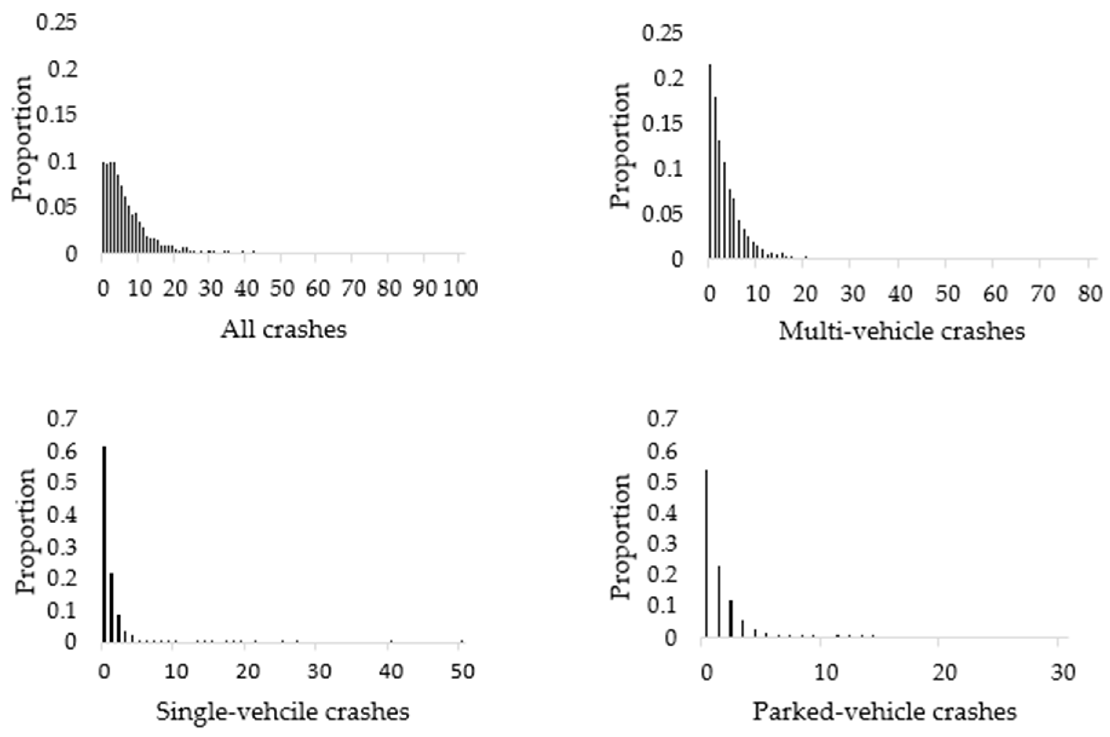
4.1. Exploratory Analysis

First, we plotted the crash counts (Figure 1) to conduct an exploratory analysis, which resulted in some crucial observations. The most important one was the proportion of zeros for different crash types, which can lead to over- or under-dispersion in the data [48] and consequently to a low sample mean. For instance, the proportions of zero counts were 9.96%, 21.62%, 61.64%, and 53.92% for all, multi-vehicle, single-vehicle, and parked vehicle crashes, respectively. While all datasets exhibited over-dispersion, single-vehicle and parked vehicle crashes appeared to have a low sample mean (see Figure 1). Given these results, special attention was directed to developing crash prediction models for single-vehicle and parked-vehicle crashes.

4.2. Modelling Results

Table 2. Generalised Poisson (GP) models by crash type.

		All Crashes	Multi-Vehicle Crashes	Single-Vehicle Crashes	Parked-Vehicle Crashes
		Coef. (St. Err.)	Coef. (St. Err.)	Coef. (St. Err.)	Coef. (St. Err.)
Generalised Poisson Model
Intercept		1.714 *** (0.240)	1.148 *** (0.287)	−0.678 (0.494)	1.267 *** (0.407)
Ln (Length)		0.474 *** (0.026)	0.557 *** (0.032)	0.565 *** (0.051)	0.642 *** (0.047)
Ln (AADT)		0.578 *** (0.017)	0.591 *** (0.021)	0.501 *** (0.036)	0.551 ** (0.027)
No of Lanes Base: one lane	Two lanes	−0.267 *** (0.054)	−0.352 *** (0.065)	-	−0.163 * (0.092)
	Three or more lanes	−0.386 *** (0.073)	−0.387 *** (0.088)	-	−0.570 *** (0.139)
Lane width		−0.113 *** (0.043)	−0.141 *** (0.051)	-	−0.081 * (0.074)
Parking Type Base: No parking	Parallel Parking	0.323 *** (0.042)	0.528 *** (0.052)	−0.318 *** (0.075)	0.949 * (0.094)
	Others a	0.350 *** (0.081)	0.633 *** (0.096)	−0.344 ** (0.168)	1.133 *** (0.137)
Speed Base: 30 km/h	50 km/h	−0.148 *** (0.045)	−0.160 *** (0.053)	-	−0.176 ** (0.073)
	70 km/h or more	−0.773 *** (0.084)	−0.839 *** (0.102)	−0.555 *** (0.149)	−1.377 *** (0.209)
Divided roadway Base: undivided		−0.312 *** (0.051)	−0.292 *** (0.062)	−0.286 *** (0.094)	−0.411 *** (0.102)
Dispersion		0.565 (0.010)	0.507 (0.012)	0.231 (0.019)	0.227 (0.018)

***: p < 0.001, **: p < 0.01, *: p < 0.1, ^a Others: Perpendicular/Angled/Mixed Parking.

and

Table 3. Negative Binomial (NB) models by crash type.

		All Crashes	Multi-Vehicle Crashes	Single-Vehicle Crashes	Parked-Vehicle Crashes
		Coef. (St. Err.)	Coef. (St. Err.)	Coef. (St. Err.)	Coef. (St. Err.)
Negative Binomial Model
Intercept		2.150 *** (0.257)	1.436 *** (0.314)	−0.380 (0.498)	1.580 *** (0.425)
Ln (Length)		0.624 *** (0.031)	0.664 *** (0.037)	0.597 *** (0.057)	0.720 *** (0.053)
Ln (AADT)		0.584 *** (0.018)	0.504 *** (0.022)	0.554 *** (0.035)	0.443 ** (0.029)
No of Lanes Base: one lane	Two lanes	−0.287 *** (0.060)	−0.394 *** (0.074)	-	−0.213 ** (0.096)
	Three or more lanes	−0.300 ** (0.085)	−0.325 *** (0.104)	-	−0.501 *** (0.143)
Lane width		−0.181 *** (0.047)	−0.192 *** (0.057)	-	−0.140 * (0.076)
Parking Type Base: No parking	Parallel Parking	0.330 *** (0.048)	0.529 *** (0.059)	−0.458 *** (0.081)	1.005 *** (0.092)
	Others a	0.459 *** (0.090)	0.755 *** (0.108)	−0.586 *** (0.180)	1.251 *** (0.142)
Speed Base: 30 km/h	50 km/h	−0.084 * (0.049)	−0.107 ** (0.060)	-	−0.132 ** (0.078)
	70 km/h or more	−0.863 *** (0.090)	−0.906 *** (0.109)	−0.471 ** (0.161)	−1.302 *** (0.190)
Divided roadways Base: undivided		−0.320 *** (0.061)	−0.367 *** (0.074)	−0.385 *** (0.104)	−0.364 *** (0.106)
Dispersion		0.491 (0.022)	0.626 (0.033)	0.753 (0.086)	0.587 (0.063)

***: p < 0.001, **: p < 0.01, *: p < 0.1, ^a Others: Perpendicular/Angled/Mixed Parking.

provide results (only significant variables) by crash type for GP and NB models, respectively. The asterisk symbol adjacent to each coefficient shows the level of significance. The predictor variables consisted of the average annual daily traffic (AADT), segment length, the number of lanes, the average width of each lane, the presence and type of on-street parking, posted speed limit, and whether or not the roadway segment was divided. The initial list of predictors included parking arrangement and median type, but they were excluded due to multicollinearity detected by the variance inflation factor (VIF).

Crash frequency positively correlated with traffic variable ‘AADT’ and segment length in all developed models. The number of lanes was significantly associated with crash frequency in all models except for single-vehicle crashes, showing a negative association. Moreover, in the GP model for parked-vehicle crashes, the coefficient for two lanes was significant only at a 90% confidence level. The coefficient for three or more lanes was higher than for two lanes, indicating a greater reduction in crash frequency for the former than the latter. Lane width demonstrated a significant negative association with crash frequency across all crash types except for single-vehicle crashes, where the association was insignificant. On-street parking types were positively correlated with crash frequency across all crash types (all crashes, multi-vehicle, and parked vehicle crash models), with perpendicular and angled parking showing the highest increase compared to parallel parking. However, there was a negative relationship between parking type and crash frequency for single-vehicle crashes. Posted speed limit coefficients indicated a negative association with crash frequency in all models except for single-vehicle crashes at 50 km/h. Furthermore, the negative magnitude for the higher speed limits, i.e., 70 km/h or above, was higher than 50 km/h. Divided roads were associated with lower crash frequency compared to undivided roads.

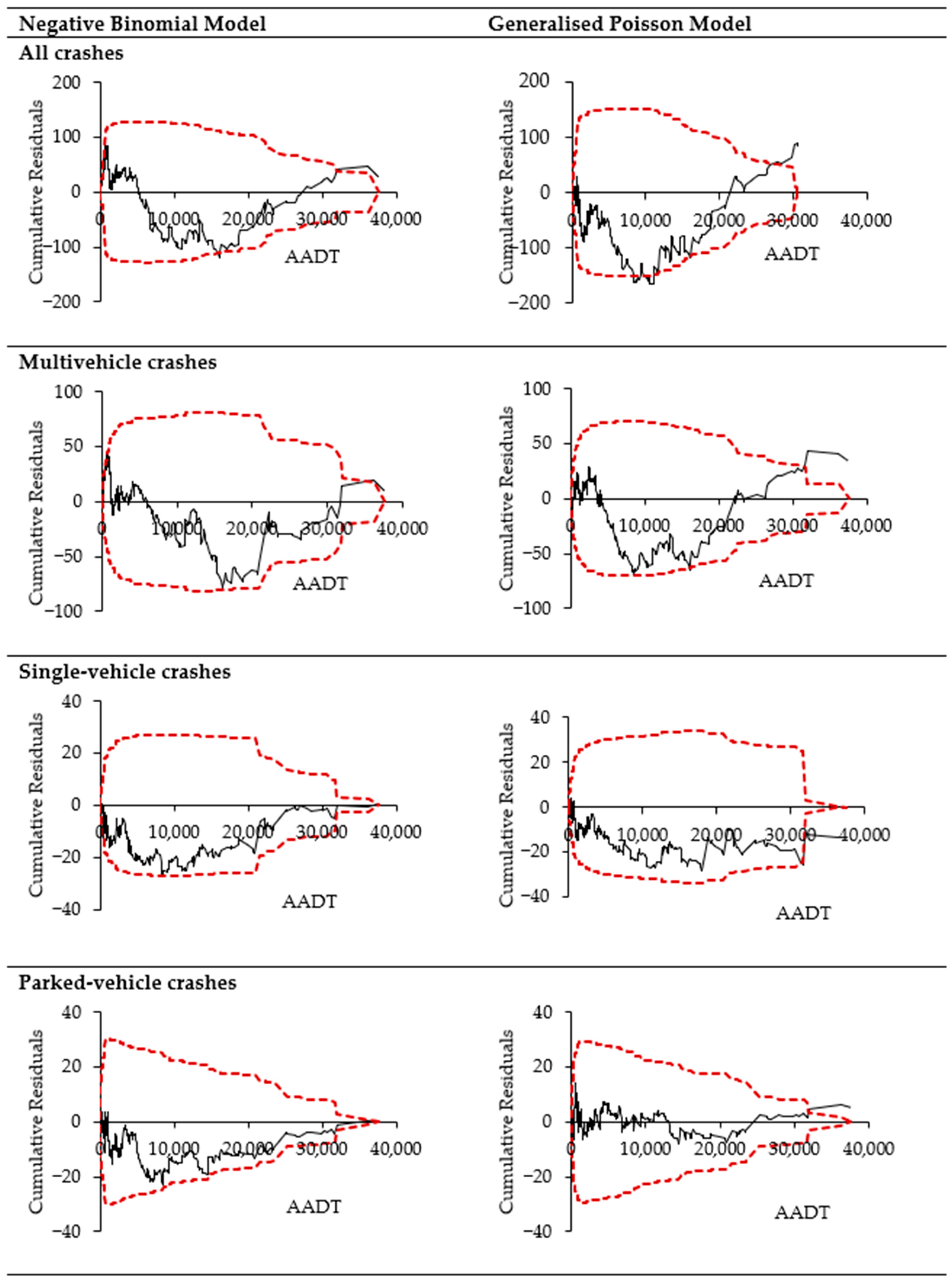
4.3. Goodness-of-Fit and Performance Evaluation

Seventy-five per cent of the data was used to develop the SPFs, and the remaining twenty-five per cent was reserved for assessing model performance. Akaike information criterion (AIC) and Bayesian information criterion (BIC) assessed the goodness of fit of the developed models where lower values of both AIC and BIC indicated better fits. For evaluating the accuracies (or predictive performance), mean prediction bias (MPB), mean absolute deviation (MAD), and mean square prediction error (MSPE), as provided in Oh et al. [55], were applied. MPB indicates the direction and magnitude of bias in model estimates, with positive values indicating overestimation and negative values indicating underestimation. The magnitude of the value indicates the average prediction bias. MAD is a measure of the difference between observed and predicted values. In this case, the positive and negative values cancel each other out, and prediction errors are only provided as positive values. The MSPE determines the quality of a predictor by measuring the expected squared difference between the predicted and actual value of the predictor. McFadden’s pseudo-R² [56] was also used to compare the competing models where the best model was selected based on the highest pseudo-R² value.

Table 4. Comparison of GP and NB models for goodness of fit and predictive performance.

	All Crashes		Multi-Vehicle Crashes		Single-Vehicle Crashes		Parked-Vehicle Crashes
	GP	NB	GP	NB	GP	NB	GP	NB
AIC	10,775.80	10,656.22	8678.63	8611.67	3985.96	4015.46	4593.96	4599.03
BIC	10,842.39	10,722.81	8745.21	8678.25	4052.491	4081.99	4660.54	4665.61
Pseudo R2	0.069	0.084	0.078	0.092	0.093	0.087	0.088	0.086
MPB	0.058	0.029	0.084	0.064	0.001	0.013	0.008	0.052
MAD	0.778	0.779	0.447	0.451	0.126	0.132	0.155	0.176
MSPE	1.872	1.728	0.726	0.699	0.385	0.450	0.054	0.061

provides the goodness of fit and performance evaluation results of GP and NB models by crash type.

Based on AIC and BIC values, NB models performed better than GP models for ‘all’ and ‘multi-vehicle’ crashes. The GP model outperformed the NB model for ‘single-vehicle’ and ‘parked-vehicle’ crashes. The pseudo-R² also revealed similar results, favouring NB models for ‘all’ and ‘multi-vehicle’ crashes and the GP models for ‘single-vehicle’ and ‘parked-vehicle’ crashes. MPB and MSPE supported NB models for ‘all’ and ‘multi-vehicle’ crashes compared to GP models. At the same time, MAD revealed virtually identical performance for the GP and NB models. The MPB, MAD, and MSPE values favoured the GP model for ‘single-vehicle’ crashes. Similarly, the values of all MPB, MAD, and MSPE supported the GP model in the case of ‘parked-vehicle’ crashes.

Moreover, Cumulative Residual (CURE) plots [57] were utilised to check the adequacy of the developed SPFs. CURE plots check the SPF-predicted values based on individual explanatory variables used in the model and provide a means to visually and objectively check which model performs better. According to Hauer [57], the closer the residuals oscillate around the zero line, the better the model fits the data. In contrast, the estimates are not considered unbiased in locations where CURE plots drift up or down substantially. Furthermore, the CURE plots for unbiased SPF lie within the boundaries of two standard deviations.

CURE plots revealed that most estimates clustered on the left side of the plots. This outcome was not unexpected, considering that a substantial portion of the road segments in the data had low traffic volume. In general, the CURE plots remained within two standard deviations for most AADT values except for the far right ends of the graphs. Overall, the obtained SPFs underestimated crash frequency for road segments with low traffic volume. However, as AADT values increased, the SPFs began to overestimate crash frequency. Furthermore, when comparing different crash types, CURE plots for ‘all’ crashes and ‘multi-vehicle’ crashes demonstrated superior performance for NB models as opposed to GP models. Conversely, CURE plots for ‘single-vehicle’ and ‘parked-vehicle’ crashes indicated that GP models performed better than NB models. These findings aligned with the results obtained from other evaluation metrics such as AIC, BIC, pseudo-R², and accuracy measures including MPB, MAD, and MSPE. Figure 2 provides the CURE plots for GP and NB models by crash type.

5. Discussion

5.1. Descriptive and Exploratory Analysis of Crash Data

The descriptive analysis of the data indicated no evidence of under-dispersion for any of the crash types, as the standard deviation values (and thus variance) exceeded the mean values for all categories. This finding aligns with the general understanding that crash data are only occasionally characterised by under-dispersion instead of over-dispersion. However, upon closer examination, it was observed that the mean values for single-vehicle crashes and crashes involving parked vehicles were relatively small (less than one). This observation served as an initial indication of a low sample mean problem within these crash types. Frequency distribution plots were constructed for each crash type to gain further insights. It was observed that the percentage of zero crash observations was relatively small for ‘all’ crashes and ‘multi-vehicle’ crashes (around 11% and 23%, respectively), which suggested that only a small proportion of road segments have zero crashes. In contrast, more than 50% of the observations had zero values for ‘single-vehicle’ crashes and crashes involving ‘parked vehicles’, implying that more than half of the road segments had zero single-vehicle or parked-vehicle crashes. This finding can be understood in light of prior research [58], which reported that most single-vehicle crashes occur in rural areas compared to urban areas. In addition, single-vehicle crashes are typically the result of driver misbehaviour, including loss of vehicle control. In contrast, multi-vehicle crashes are often associated with driver errors during interactions with other vehicles [59]. The likelihood of avoiding collision with other vehicles is typically lower in urban areas, which results in a higher frequency of multi-vehicle crashes.

To sum up, the exploratory analysis indicated that the crash data in this study did not exhibit under-dispersion but instead demonstrated a low sample mean for single-vehicle and parked-vehicle crashes.

5.2. Crash Frequency and Its Covariates

The analysis revealed several significant relationships between crash frequency and explanatory variables. For instance, there was a positive association between traffic volume and crash frequency, consistent across all models (for all crash types). Positive association means that crash frequency increases as traffic volume increases. This observation agrees with the findings of previous studies [11,23]. It is logical to assume that as the number of vehicles on the roadways increases, the likelihood of involving in a crash also increases. Similarly, longer homogenous segments were associated with higher crash frequencies. Longer segments induce monotonous traffic conditions, encouraging drivers to speed and take more risks, increasing the likelihood of crash involvement.

The relationship between crash frequency and the number of lanes was negative in all, multi-vehicle, and parked-vehicle crash models, indicating that roadways with more lanes were safer than those with fewer lanes. On the other hand, it was not significant in single-vehicle crash models. The increase in the number of lanes and the corresponding decrease in crash frequency could occur because drivers have more space to take preventive action and avoid crashes as the number of lanes increases. Moreover, fewer lanes correspond to less available space for preventative measures. Kononov et al. [60] found that adding lanes may initially result in a temporary safety improvement that disappears as congestion increases. In our study, the target roadway type is urban local roads where the speed limit and operating speed are often not very high, which offers more time for drivers to take preventive actions on wider roads (roads with many lanes). The same reasoning could also be extended to explain the negative association between lane width and crash frequency.

The presence of on-street parking showed a positive association with crash frequency, indicating that crash frequency rises when there is on-street parking, regardless of its type. However, the increase in crash frequency was notably high when perpendicular and angled parking types were present. Since angle and perpendicular parking require relatively complex manoeuvres, we were not surprised to observe an increase in crash frequency for those parking types. Similar results are frequently reported in the literature [61,62]; however, on-street parking leads to a reduced frequency of single-vehicle crashes, which is understandable. When vehicles are parked, drivers typically exercise more caution compared to cases when roads are without parked vehicles; even when there is a collision, it cannot be classified as a single-vehicle crash.

The developed models showed a negative association between crash frequency and speed limits, which was initially surprising. However, similar results were reported by Liu et al. [23]. In Belgium, authorities continuously assess the safety situations of roadway facilities and propose changes to the speed regimes if necessary (for example, see [63] for the latest updates). It is plausible that the lower speed limits were implemented for segments (when data were collected) that previously had a higher number of observed crashes. Consequently, the lower speed limit segments might appear less safe in the models than those with higher speed limits. This suggests that the negative association between crash frequency and higher speed limits, as indicated by model coefficients, may not necessarily be due to a positive effect of higher speed limits on safety. Rather, it could be attributed to the changes or reductions in the posted speed limit specifically for the segments with a history of crashes, which could explain this negative correlation. In addition, our data only referred to the design speed limit, not operational speed. Intini et al. [64] found that inferred operating speeds comparable to or higher than the inferred design speed present recurrent safety issues. As expected, the relationship between crash frequency and divided roadways was negative. Divided roads reduce the chances of direct conflict with vehicles, particularly those approaching from the opposite direction. Consequently, divided roadways experience fewer collisions than undivided roadways, as revealed by the estimated coefficients in both GP and NB models. These results confirm the findings of Williams et al. [65], who indicated that roadways with raised medians in urban areas are safer than undivided roadways.

5.3. Performance Comparison

Our findings indicated that the NB model performed relatively better than GP models when considering total and multi-vehicle crashes. However, the GP model exhibited a better fit than NB models for single-vehicle and parked-vehicle crashes (crash types characterised by a low sample mean). In other words, the GP model performed better for crash types with distributions with a small sample mean and resulting long right tail due to a substantial number of zero observations and only a few smaller values for other observations (road segments). This result aligns with the recommendations by Joe and Zhu [51], who suggested using GP regression for modelling distributions exhibiting long right tails. The finding about the GP model’s superior performance for crash types characterised by a low sample mean (and long right tails) is a valuable outcome of this study. We recommend that researchers check both NB and GP models for adequacy, particularly when analysing crash data with a low sample mean. Neglecting to check the GP model may lead to less accurate estimates. Utilising the GP model for datasets with low sample mean could achieve better goodness of fit and predictive performance than the traditional NB model. To sum up, these findings highlight the importance of model selection based on the specific characteristics of the dataset at hand.

5.4. Practical Significance

Accurate crash prediction and information about predictor variables can help identify sites where crashes are more likely to occur. By detecting these locations, transportation authorities can implement targeted preventative measures. These may include installing traffic calming devices for effective traffic management, adding lanes or widening existing ones to enhance safety, improving road signage, enhancing visibility to mitigate the increased crash frequency associated with on-street parking, or implementing speed limit adjustments. By taking these steps, the likelihood of crashes happening could be significantly reduced. In addition, accurate crash prediction models enable funding agencies and transportation departments to allocate resources more effectively. By focusing on sites or segments of the transportation network where higher frequency is estimated, resources such as funding for infrastructure improvements, traffic enforcement, and safety campaigns can be directed to where they are most needed. This targeted approach maximises the impact of interventions, resulting in more efficient resource utilisation and improved road safety outcomes. Government agencies and policymakers utilise accurate crash prediction models to shape transportation policies and regulations at a planning level. These models provide valuable insights into the influence of various infrastructure-related variables on crash frequency, allowing policymakers to assess their impact on road safety outcomes. For instance, by analysing crash prediction data, policymakers can identify trends, patterns, and risk factors contributing to crashes, informing evidence-based decision-making. This includes decisions related to transportation infrastructure investments, road design standards, traffic management strategies, and public safety initiatives. Crash prediction models serve as valuable tools for evaluating the effectiveness of existing interventions to enhance road safety. By comparing predicted crash rates with actual crash data, policymakers can assess whether implemented measures achieve the desired outcomes. This evaluation process facilitates the iterative improvement of policies and interventions, ensuring that resources are allocated to initiatives with the most significant potential to reduce crashes and save lives. However, for this, the accuracy of crash prediction is crucial. By identifying risk factors and patterns of crashes (e.g., increase or decrease in expected frequency of certain crash types), crash prediction models help policymakers anticipate future needs and develop strategies to mitigate risks at the planning stage.

5.5. Limitations and Future Research

Inevitably, this study has its limitations. We only focused on crash data for urban road segments. Future studies are encouraged to further explore the adequacy of GP models for distributions with low sample means in other conditions, e.g., rural roads, motorways, or urban arterials. Developing GP models for different crash types and severity levels should also be pursued. Besides the given variables, future studies are encouraged to explore the impact of driveway density, the intersection (crossroad or unsignalised intersection) density, and the presence and type of bicycle lanes on crash prediction in urban areas. Interested readers are referred to these studies for the whole list of potential predictors [22,66,67]. Moreover, NB and GP regression models offer different mean–variance relationships in NB-1, NB-2 and NB-P functional forms [50] or GP-1, GP-2 or GP-P functional forms [44]. Therefore, these mean–variance relationships were not examined in the current study and are left for future studies. Further research should also investigate the application of GP models in the empirical Bayes method and hotspot identification. It is worth noting that this study focused solely on point estimation of crashes, suggesting that developing interval estimates of crash frequency could be an exciting avenue for future research.

6. Conclusions

By applying the GP model, the study developed crash prediction models to examine the association between crash frequency and road infrastructure elements in the urban areas, specifically those related to the cross-section design of road segments. The literature on the association between crash frequency and explanatory variables shows confusing and somewhat contradictory findings in urban areas. Moreover, the NB models, typically applied to analyse crash data, have limitations in effectively modelling datasets characterised by low sample means and under-dispersion (although the latter was not observed in the current study). On the other hand, GP models show the capacity to handle such distributions effectively. Considering these gaps, this study estimated crash prediction models for urban road segments using GP models and identified these complex relationships for different crash types, including total crashes, multi-vehicle crashes, single-vehicle crashes, and parked-vehicle crashes. The study also developed corresponding NB models and evaluated GP and NB models for goodness of fit and predictive performance. As expected, the findings revealed numerous significant relationships between crash frequency and explanatory variables. The most important predictor of road crashes was traffic volume, which was significant in all models. All, multi-vehicle, and parked vehicle crash models showed different significant predictors compared to single-vehicle models. While the NB model outperformed GP models in the case of ‘all’ crashes and ‘multi-vehicle crashes’, the GP model’s performance was superior to that of the corresponding NB models for ‘single-vehicle’ and ‘parked-vehicle’. Crashes. Overall, the findings highlight the potential of GP models as an alternative to NB models in analysing crash data characterised by a low sample mean, as applying GP models could lead to improved fit and predictive performance, providing more accurate estimates in the analysis of crash data. From a practical perspective, GP models offer practitioners and authorities a balance of interpretability and predictive power compared to complex models, making them easier to implement in real-world road safety situations.

References

1. Nassiri, H.; Mohamadian Amiri, A.; Najaf, P.; Mohamadian Amiri, A. Prediction of Roadway Accident Frequencies: Count Regressions versus Machine Learning Models. Sci. Iran. 2014, 21, 263–275. [Google Scholar]
2. Swedish Parliament. Nollvisionen Och Det Trafiksäkra Samhället (Vision Zero and the Road Traffic Safety Society); Sveriges Riksdag: Stockholm, Sweden, 1997.
3. Belin, M.-Å.; Tillgren, P.; Vedung, E. Vision Zero—A Road Safety Policy Innovation. Int. J. Inj. Control Saf. Promot. 2012, 19, 171–179. [Google Scholar] [CrossRef]
4. Al-Rousan, T.M.; Umar, A.A.; Al-Omari, A.A. Characteristics of Crashes Caused by Distracted Driving on Rural and Suburban Roadways in Jordan. Infrastructures 2021, 6, 107. [Google Scholar] [CrossRef]
5. Chhotu, A.K.; Suman, S.K. Prediction of Fatalities at Northern Indian Railways’ Road–Rail Level Crossings Using Machine Learning Algorithms. Infrastructures 2023, 8, 101. [Google Scholar] [CrossRef]
6. Pirdavani, A.; Brijs, T.; Bellemans, T.; Wets, G. Evaluation of Traffic Safety at Un-Signalized Intersections Using Microsimulation: A Utilisation of Proximal Safety Indicators. Adv. Transp. Stud. 2010, 22, 43–50. [Google Scholar]
7. Nikolaou, D.; Dragomanovits, A.; Ziakopoulos, A.; Deliali, A.; Handanos, I.; Karadimas, C.; Kostoulas, G.; Frantzola, E.K.; Yannis, G. Exploiting Surrogate Safety Measures and Road Design Characteristics towards Crash Investigations in Motorway Segments. Infrastructures 2023, 8, 40. [Google Scholar] [CrossRef]
8. Miaou, S.-P.; Lord, D. Modeling Traffic Crash-Flow Relationships for Intersections: Dispersion Parameter, Functional Form, and Bayes Versus Empirical Bayes Methods. Transp. Res. Rec. 2003, 1840, 31–40. [Google Scholar] [CrossRef]
9. Pirdavani, A.; Brijs, T.; Bellemans, T.; Kochan, B.; Wets, G. Application of Different Exposure Measures in Development of Planning-Level Zonal Crash Prediction Models. Transp. Res. Rec. 2012, 2280, 145–153. [Google Scholar] [CrossRef]
10. Zhang, Z.; Liu, J.; Li, X.; Fu, X.; Yang, C.; Jones, S. Localizing Safety Performance Functions for Two-Way STOP-Controlled (TWST) Three-Leg Intersections on Rural Two-Lane Two-Way (TLTW) Roadways in Alabama: A Geospatial Modeling Approach with Clustering Analysis. Accid. Anal. Prev. 2023, 179, 106896. [Google Scholar] [CrossRef]
11. Kim, J.; Anderson, M.; Gholston, S. Modeling Safety Performance Functions for Alabama’s Urban and Suburban Arterials. Int. J. Traffic Transp. Eng. 2015, 4, 84–93. [Google Scholar]
12. Jin, W.; Chowdhury, M.; Mahmud Khan, S.; Gerard, P. Investigating the Impacts of Crash Prediction Models on Quantifying Safety Effectiveness of Adaptive Signal Control Systems. J. Saf. Res. 2021, 76, 301–313. [Google Scholar] [CrossRef]
13. Gitelman, V.; Carmel, R.; Doveh, E.; Hakkert, S. Exploring Safety Impacts of Pedestrian-Crossing Configurations at Signalized Junctions on Urban Roads with Public Transport Routes. Int. J. Inj. Control Saf. Promot. 2018, 25, 31–40. [Google Scholar] [CrossRef]
14. El-Basyouny, K.; Sayed, T. Measuring Direct and Indirect Treatment Effects Using Safety Performance Intervention Functions. Saf. Sci. 2012, 50, 1125–1132. [Google Scholar] [CrossRef]
15. Highway Safety Manual (HSM); AASHTO, American Association of State and Highway Transportation Officials: Washington DC, USA, 2010; ISBN 978-1-56051-477-0.
16. Mendes, O.B.B.; Larocca, A.P.C.; Rodrigues Silva, K.; Pirdavani, A. Assessing the Performance of Highway Safety Manual (HSM) Predictive Models for Brazilian Multilane Highways. Sustainability 2023, 15, 10474. [Google Scholar] [CrossRef]
17. Lu, J.; Haleem, K.; Alluri, P.; Gan, A.; Liu, K. Developing Local Safety Performance Functions versus Calculating Calibration Factors for SafetyAnalyst Applications: A Florida Case Study. Saf. Sci. 2014, 65, 93–105. [Google Scholar] [CrossRef]
18. Persaud, B.; Saleem, T.; Faisal, S.; Lyon, C.; Chen, Y.; Sabbaghi, A. Adoption of Highway Safety Manual Predictive Technologies for Canadian Highways. In Proceedings of the 2012 Conference and Exhibition of the Transportation Association of Canada—Transportation: Innovations and Opportunities, Fredericton, NB, Canada, 14–17 October 2012. [Google Scholar]
19. Kaaf, K.A.; Abdel-Aty, M. Transferability and Calibration of Highway Safety Manual Performance Functions and Development of New Models for Urban Four-Lane Divided Roads in Riyadh, Saudi Arabia. Transp. Res. Rec. 2015, 2515, 70–77. [Google Scholar] [CrossRef]
20. Vieira Gomes, S. The Influence of the Infrastructure Characteristics in Urban Road Accidents Occurrence. Accid. Anal. Prev. 2013, 60, 289–297. [Google Scholar] [CrossRef]
21. Khattak, M.W.; Pirdavani, A.; De Winne, P.; Brijs, T.; De Backer, H. Estimation of Safety Performance Functions for Urban Intersections Using Various Functional Forms of the Negative Binomial Regression Model and a Generalized Poisson Regression Model. Accid. Anal. Prev. 2021, 151, 105964. [Google Scholar] [CrossRef]
22. Brijs, T.; Pirdavani, A. Urban and Suburban Arterials. In Safe Mobility: Challenges, Methodology and Solutions; Transport and Sustainability; Lord, D., Washington, S., Eds.; Emerald Publishing Limited: Bingley, UK, 2018; Volume 11, pp. 85–106. ISBN 978-1-78635-223-1. [Google Scholar]
23. Liu, C.; Zhao, M.; Li, W.; Sharma, A. Multivariate Random Parameters Zero-Inflated Negative Binomial Regression for Analysing Urban Midblock Crashes. Anal. Methods Accid. Res. 2018, 17, 32–46. [Google Scholar] [CrossRef]
24. Park, J.; Abdel-Aty, M. Evaluation of Safety Effectiveness of Multiple Cross Sectional Features on Urban Arterials. Accid. Anal. Prev. 2016, 92, 245–255. [Google Scholar] [CrossRef]
25. Barua, S.; El-Basyouny, K.; Islam, M.T. Safety Performance Functions to Assess the Safety Risk of Urban Residential Collector Roads. In Proceedings of the Technical Session of the 2014 Conference of the Transportation Association of Canada, Montreal, QC, Canada, 28 September–1 October 2014. [Google Scholar]
26. Khattak, M.W.; De Backer, H.; De Winne, P.; Brijs, T.; Pirdavani, A. Analysis of Factors Influencing Road Crashes in the Urban Areas: The Application of Generalised Poisson Model vs Negative Binomial Model. In Proceedings of the 6th International Symposium on Highway Geometric Design (ISHGD), Amsterdam, The Netherlands, 26–29 June 2022. [Google Scholar]
27. Vieira Gomes, S.; Cardoso, J.L. Estimativa de Frequências de Acidentes Rodoviários em Meio Urbano Considerando Volumes de Tráfego de Peões; Departamento de Transportes Núcleo de Planeamento, Tráfego e Segurança, Laboratório Nacional de Engenharia Civil: Lisbon, Portugal, 2008. [Google Scholar]
28. Potts, I.B.; Harwood, D.W.; Richard, K.R. Relationship of Lane Width to Safety on Urban and Suburban Arterials. Transp. Res. Rec. 2007, 2023, 63–82. [Google Scholar] [CrossRef]
29. Rista, E.; Goswamy, A.; Wang, B.; Barrette, T.; Hamzeie, R.; Russo, B.; Bou-Saab, G.; Savolainen, P.T. Examining the Safety Impacts of Narrow Lane Widths on Urban/Suburban Arterials: Estimation of a Panel Data Random Parameters Negative Binomial Model. J. Transp. Saf. Secur. 2018, 10, 213–228. [Google Scholar] [CrossRef]
30. Sharma, A.; Li, W.; Zhao, M.; Rilett, L. Safety and Operational Analysis of Lane Widths in Mid-Block Segments and Intersection Approaches in the Urban Environment in Nebraska; Research Reports; Nebraska Department of Transportation: Lincoln, NE, USA, 2015.
31. Khodadadi, A.; Shirazi, M.; Geedipally, S.; Lord, D. Evaluating Alternative Variations of Negative Binomial–Lindley Distribution for Modelling Crash Data. Transp. A Transp. Sci. 2023, 19, 2062480. [Google Scholar] [CrossRef]
32. Geedipally, S.R.; Lord, D.; Dhavala, S.S. The Negative Binomial-Lindley Generalized Linear Model: Characteristics and Application Using Crash Data. Accid. Anal. Prev. 2012, 45, 258–265. [Google Scholar] [CrossRef]
33. Zhang, Y.; Ye, Z.; Lord, D. Estimating Dispersion Parameter of Negative Binomial Distribution for Analysis of Crash Data: Bootstrapped Maximum Likelihood Method. Transp. Res. Rec. 2007, 2019, 15–21. [Google Scholar] [CrossRef]
34. Lord, D.; Mannering, F. The Statistical Analysis of Crash-Frequency Data: A Review and Assessment of Methodological Alternatives. Transp. Res. Part A Policy Pract. 2010, 44, 291–305. [Google Scholar] [CrossRef]
35. Saha, K.; Paul, S. Bias-Corrected Maximum Likelihood Estimator of the Negative Binomial Dispersion Parameter. Biometrics 2005, 61, 179–185. [Google Scholar]
36. Hardin, J.W.; Hilbe, J. Generalized Linear Models and Extensions, 2nd ed.; Stata Press: College Station, TX, USA, 2007; ISBN 978-1-59718-014-6. [Google Scholar]
37. Lord, D.; Geedipally, S.R.; Guikema, S.D. Extension of the Application of Conway-Maxwell-Poisson Models: Analysing Traffic Crash Data Exhibiting Underdispersion. Risk Anal. 2010, 30, 1268–1276. [Google Scholar] [CrossRef]
38. Lord, D. Modeling Motor Vehicle Crashes Using Poisson-Gamma Models: Examining the Effects of Low Sample Mean Values and Small Sample Size on the Estimation of the Fixed Dispersion Parameter. Accid. Anal. Prev. 2006, 38, 751–766. [Google Scholar] [CrossRef]
39. Maher, M.J.; Summersgill, I. A Comprehensive Methodology for the Fitting of Predictive Accident Models. Accid. Anal. Prev. 1996, 28, 281–296. [Google Scholar] [CrossRef]
40. Park, B.-J.; Lord, D.; Hart, J.D. Bias Properties of Bayesian Statistics in Finite Mixture of Negative Binomial Regression Models in Crash Data Analysis. Accid. Anal. Prev. 2010, 42, 741–749. [Google Scholar] [CrossRef]
41. Pew, T.; Warr, R.L.; Schultz, G.G.; Heaton, M. Justification for Considering Zero-Inflated Models in Crash Frequency Analysis. Transp. Res. Interdiscip. Perspect. 2020, 8, 100249. [Google Scholar] [CrossRef]
42. Lord, D.; Washington, S.; Ivan, J.N. Further Notes on the Application of Zero-Inflated Models in Highway Safety. Accid. Anal. Prev. 2007, 39, 53–57. [Google Scholar] [CrossRef]
43. Consul, P.C.; Famoye, F. Generalized Poisson Regression Model. Commun. Stat. Theory Methods 1992, 21, 89–109. [Google Scholar] [CrossRef]
44. Zamani, H.; Ismail, N. Functional Form for the Generalised Poisson Regression Model. Commun. Stat. Theory Methods 2012, 41, 3666–3675. [Google Scholar] [CrossRef]
45. Ismail, N.; Jemain, A.A. Handling Overdispersion with Negative Binomial and Generalised Poisson Regression Models. Casualty Actuar. Soc. Forum 2007, 2007, 103–158. Available online: https://www.casact.org/sites/default/files/database/forum_07wforum_07w109.pdf (accessed on 1 January 2024).
46. Ndue, K.; Baylie, M.M.; Goda, P. Determinants of Rural Households’ Intensity of Flood Adaptation in the Fogera Rice Plain, Ethiopia: Evidence from Generalised Poisson Regression. Sustainability 2023, 15, 11025. [Google Scholar] [CrossRef]
47. Wu, P.; Li, J.; Pian, Y.; Li, X.; Huang, Z.; Xu, L.; Li, G.; Li, R. How Determinants Affect Transfer Ridership between Metro and Bus Systems: A Multivariate Generalized Poisson Regression Analysis Method. Sustainability 2022, 14, 9666. [Google Scholar] [CrossRef]
48. Yadav, B.; Jeyaseelan, L.; Jeyaseelan, V.; Durairaj, J.; George, S.; Selvaraj, K.G.; Bangdiwala, S.I. Can Generalized Poisson Model Replace Any Other Count Data Models? An Evaluation. Clin. Epidemiol. Glob. Health 2021, 11, 100774. [Google Scholar] [CrossRef]
49. Famoye, F.; Wulu, J.T.; Singh, K.P. On the Generalised Poisson Regression Model with an Application to Accident Data. J. Data Sci. 2004, 2, 287–295. [Google Scholar] [CrossRef]
50. Greene, W. Functional Forms for the Negative Binomial Model for Count Data. Econ. Lett. 2008, 99, 585–590. [Google Scholar] [CrossRef]
51. Joe, H.; Zhu, R. Generalized Poisson Distribution: The Property of Mixture of Poisson and Comparison with Negative Binomial Distribution. Biom. J. 2005, 47, 219–229. [Google Scholar] [CrossRef]
52. Hubert, P.C., Jr.; Lauretto, M.S.; Stern, J.M. FBST for Generalized Poisson Distribution. AIP Conf. Proc. 2009, 1193, 210–217. [Google Scholar] [CrossRef]
53. Yang, Z.; Hardin, J.W.; Addy, C.L.; Vuong, Q.H. Testing Approaches for Overdispersion in Poisson Regression versus the Generalized Poisson Model. Biom. J. 2007, 49, 565–584. [Google Scholar] [CrossRef]
54. Ye, F.; Wang, Y. Performance Evaluation of Various Missing Data Treatments in Crash Severity Modeling. Transp. Res. Rec. 2018, 2672, 149–159. [Google Scholar] [CrossRef]
55. Oh, J.; Lyon, C.; Washington, S.; Persaud, B.; Bared, J. Validation of FHWA Crash Models for Rural Intersections: Lessons Learned. Transp. Res. Rec. 2003, 1840, 41–49. [Google Scholar] [CrossRef]
56. McFadden, D. Conditional Logit Analysis of Qualitative Choice Behavior. In Frontiers in Econometrics; Academic Press: Cambridge, MA, USA, 1974. [Google Scholar]
57. Hauer, E. The Art of Regression Modeling in Road Safety; Springer International Publishing: Cham, Switzerland, 2015; ISBN 978-3-319-12528-2. [Google Scholar]
58. Chen, H.Y.; Ivers, R.Q.; Martiniuk, A.L.C.; Boufous, S.; Senserrick, T.; Woodward, M.; Stevenson, M.; Williamson, A.; Norton, R. Risk and Type of Crash among Young Drivers by Rurality of Residence: Findings from the DRIVE Study. Accid. Anal. Prev. 2009, 41, 676–682. [Google Scholar] [CrossRef]
59. Dong, B.; Ma, X.; Chen, F.; Chen, S. Investigating the Differences of Single-Vehicle and Multivehicle Accident Probability Using Mixed Logit Model. J. Adv. Transp. 2018, 2018, e2702360. [Google Scholar] [CrossRef]
60. Kononov, J.; Bailey, B.; Allery, B.K. Relationships between Safety and Both Congestion and Number of Lanes on Urban Freeways. Transp. Res. Rec. 2008, 2083, 26–39. [Google Scholar] [CrossRef]
61. Box, P.C. Angle Parking Issues Revisited, 2001. ITE J. 2002, 72, 36–47. [Google Scholar]
62. Moran, M.E. What’s Your Angle? Analysing Angled Parking via Satellite Imagery to Aid Bike-Network Planning. Environ. Plan. B Urban Anal. City Sci. 2021, 48, 1912–1925. [Google Scholar] [CrossRef]
63. Boelaert, F. Afwegingskader Voor Het Invoeren van 30 km/u op Gewest- en Gemeentewegen Binnen de Bebouwde Kom; Vlaamse Overheid, Departement Mobiliteit en Openbare, Werken; Agentschap Wegen en Verkeer. 2021. Available online: https://assets.vlaanderen.be/image/upload/v1638886808/Afwegingskader_3050_hsjju2.pdf (accessed on 1 January 2024).
64. Intini, P.; Berloco, N.; Ranieri, V.; Colonna, P. Geometric and Operational Features of Horizontal Curves with Specific Regard to Skidding Proneness. Infrastructures 2020, 5, 3. [Google Scholar] [CrossRef]
65. Williams, K.M.; Stover, V.G.; Dixon, K.K.; Demosthenes, P. Access Management Manual; Transportation Research Board (TRB): Washington, DC, USA, 2014; ISBN 0-309-29541-6. [Google Scholar]
66. Harwood, D.W.; Council, F.M.; Hauer, E.; Hughes, W.E.; Vogt, A. Prediction of the Expected Safety Performance of Rural Two-Lane Highways; Federal Highway Administration: Washington, DC, USA, 2000; p. 1997.
67. Russo, F.; Busiello, M.; Dell Acqua, G. Safety Performance Functions for Crash Severity on Undivided Rural Roads. Accid. Anal. Prev. 2016, 93, 75–91. [Google Scholar] [CrossRef]
Figure 1. Crash frequency by type.
Infrastructures 09 00047 g001
Figure 2. Cumulative Residual (CURE) plots NB Model (left) and GP Model (right).
Infrastructures 09 00047 g002