Numerical Modeling of Cracked Arch Dams. Effect of Open Joints during the Construction Phase

Abstract

Running a numerical model for a cracked arch dam that takes into account all the particularities of the materials and dam with a high level of detail has a great computational cost involved. For this reason, it is usual to simplify such a model in search of a simpler solution while preserving the characteristic of being representative, with all the particularities that the model of an arch dam has. A common simplification lies in not considering open transverse joints in the construction phase of a cracked dam. An aim of this study is to propose a methodology that combines open joints and cracking, something on which, to the authors’ knowledge, no studies have been published. An additional goal is a study of the need and adequacy of different approaches on performance (computational time) and its consequences for model accuracy. For this purpose, an accurate methodology for a stationary finite element method numerical simulation of deformations in cracked arch dams is presented. Using a tetrahedron mesh of a real dam, different simplifications commonly used in numerical models are compared. It is concluded that some of the standard simplifications produce a significant effect on the computation time and accuracy of the results.

1. Introduction

Dams are essential infrastructure in the management of water resources, as they are fundamental to harnessing, regulating, and allocating water for various human needs. These engineered structures serve as the backbone for the provision of essential services, including flood control, water supply, agricultural irrigation, hydropower generation, and recreational opportunities. The fundamental importance of dams goes beyond their immediate functions and has significant economic, environmental, and social impacts. However, the benefits derived from dams can sometimes be diminished by the inherent risks they pose to downstream populations and property [1]. According to the International Commission on Large Dams (ICOLD), the number of large dams built worldwide exceeds 57,000 [2] (a large dam is defined by the ICOLD as a dam with a height of 15 m or greater from lowest foundation to crest or a dam between 5 m and 15 m impounding more than 3 million cubic meters [3]).

The technical complexities inherent in the life cycles of dams pose a number of formidable challenges covering their design, construction, operation, and eventual decommissioning. Engineers responsible for managing dams, with dams being massive structures designed to manage water resources, face a myriad of technical difficulties that require meticulous consideration and resolution. Throughout their operational life, dams face continuous challenges related to sedimentation, environmental impacts, seepage (the process of water leaking out), and maintenance. All of these pose a continuous threat to their functionality and safety, requiring constant monitoring, treatment, and adaptive management strategies. This means that, in some dams, aging is occurring faster than expected, even reaching a critical degree of degradation [4].

Therefore, it is necessary to pay close attention to the design, performance, and maintenance of a dam to ensure its reliability, safety, and stability, and to minimize the likelihood of major failures [5]. The American Society of Civil Engineers report classifies the risks of dams as (i) high (potentially causing human losses), (ii) significant (economic losses), (iii) low, and (iv) undetermined. Approximately 17% and 12% of dams fall into each of the first two categories [6], making structural condition monitoring essential to protect dam structures.

As is recognized, dam engineering problems are among the most complex in civil engineering [7], not only because of their particular geometry, but also because of the interaction of different material phases (e.g., solid–fluid); the fact that the construction material changes continuously over time (concrete, asphalt membranes, permeability of earth dams, etc.); being surrounded by a large amount of material, which causes a higher degree of heterogeneity; and, finally, because of the diverse nature of the applied loads (self-weight, water pressure, thermal, seepage, ice, wind, seismic…).

Several studies exist on cracked arch dam calculations using nonlinear finite elements in which, generally, each element can move to a cracked state (indicating the location of the crack) as a result of deformations and some formulation [8,9,10,11,12]. There are also many studies on arch dam calculations considering transverse joints between cantilevers, where each dam cantilever behaves in a linear elastic way, although the dam as a whole is nonlinear since it includes transverse construction joints that can be opened freely under friction, for which a nonlinear element is designed as a joint between the faces of the cantilevers in contact [13,14]. Some other studies compare the latter approach against a monolithic dam, where joints can never open [15,16]. Reviews of the simulations of arch dams have already been conducted, pointing out if the construction joints are taken into account [17].

But it is not common practice to combine both (open joints in the construction phase and cracks) in the same analysis. Running a numerical model that takes into account all the particularities of the materials, joints, cracking, etc., with a high level of detail is not feasible due to the computational cost involved. For this reason, it is common to propose simplifications in the models in search of a simpler solution but preserving the characteristic of being representative. Furthermore, it must be taken into account that different simulation packages, commercial or not, provide different options for modeling structures, which are not always equivalent (for example, different FEM—finite element method—programs implement different mathematical models for materials).

This study pursues two goals, the first is to develop a realistic FEM methodology that combines self-weight computation, taking into account open transverse joints with a crack appearing after joint sealing, something about which, to the authors’ knowledge, no study has been published. The second objective is to study different approaches to simplifications in numerical models in terms of computational cost and model accuracy.

2. Methods

2.1. General Approach

In the course of this paper, a numerical experimentation campaign on a case study is performed in order to determine the influence of simplifications on the deformation results of a cracked dam. This campaign is divided into five stages (Figure 1): (i) develop a numerical simulation methodology with sufficient accuracy for the requirements of the study, (ii) perform the necessary tests for the starting parameters, (iii) calibrate the material parameters, (iv) compare the results of the simplifications with the first crack, and (v) compare the results of the simplifications with the second crack.

2.2. Numerical Approach

In the first place, to solve the simulations of the dam-foundation environment required in this study, advanced numerical methods of the FEM type are used, ruling out the following factors:

• Models involving nonlinear materials;
• Transient models;
• Thermal effect;
• Analysis of the separation between the dam and the ground.

The above factors are not included in this work due to the fact that they do not directly affect the main scope of this study (i.e., deformations of dams after cracking) and because their inclusion would greatly complicate the numerical calculations, increasing the time required for calculation and the range of different options available, thus making a comparison unfeasible. Furthermore, it should be mentioned that the results of circumferential displacements and radial stresses are not analyzed in the study because they are not relevant factors in the behavior of a cracked arch dam.

In the same way, it is considered as one of the possible simplifications not to consider the transverse joints between cantilevers in the simulations, i.e., to consider the dam as a monolithic structure before applying any load. However, as will be shown in Section 4.1.2, the effect of omitting transverse joints is not negligible.

The boundary conditions applied to the simulated models consist of constraining any type of movement at the lower base of the bedrock as well as constraining horizontal movements at the sides of the bedrock. The volume of soil modeled is considered sufficient so that the applied constraints do not affect the results obtained.

The Ansys Mechanical Finite Element Analysis Software (Version R2) for Structural Engineering 2022 R2 [18] and 3D designs are used to perform all these numerical simulations. All simulations are performed with the Mechanical APDL solver. For the simulations with friction surfaces, the iterative solver Preconditioned Conjugate Gradient is used with a tolerance value of 10⁻⁸, maximum number of substeps equal to 4, and maximum number of iterations equal to the number of nodes times the degrees of freedom of each node.

2.3. Calibration

In order to be able to compare the results of the simulations with the actual monitoring measurements, it is important to take into account that the properties of the concrete and the soil may have changed since the construction work was completed.

The aim of this research is to study the numerical modeling and, as already mentioned, the thermal effect is not taken into account to avoid unnecessarily increasing the complexity of the problem. Therefore, to facilitate the elimination of the thermal effect, a dam was chosen (as will be seen later) with a north–south orientation, which greatly favors this approach by causing thermal symmetry [19]. Under this premise, it is possible to obtain real data to use as a basis for the calibration, eliminating the influence of the thermal effect on the movements. With the purpose of discarding the thermal effect from the data used, the increase in deformations of the dam is determined between two dates with equivalent thermal load. Assuming, in this way, that all the deformation variation between these dates is due to the change in hydrostatic pressure, it is possible to compare the monitoring records of the dam with the numerical simulation results.

Then, to select the dates with the same thermal load, the air temperature records at the dam weather station were consulted by comparing the average temperature for the same pair of months as those of the original transverse-joint sealing (March and April) over the years. This comparison resulted in the two possible pairs of dates shown in

Table 1. Average air temperature in °C.

	1990	1991	2006	2007
March	8.97	8.90	7.99	7.88
April	8.94	8.68	11.70	12.08

. It was decided to use the first pair to calibrate since the reservoir level variation is higher in that pair of dates.

Lastly, a calibration process is performed by the centroid method [20], involving the following steps:

• A range of values of the studied properties is set, with some exploration values for each one. Initially, the design values are used, with the addition of several higher values. The exploration points are the pairs that result from the combination of these values.
• The error is calculated in each case by comparing simulations with the auscultation records of the devices that record the greatest movements (the three upper three of the central cantilevers). The following is used as an error calculation formula: ${\sum }_{i=1}^6{\left(-1+\raisebox{1ex}{$u_i$}\!\left/ \!\raisebox{-1ex}{$u_{i.obj}$}\right.\right)}^2$. With i the points where the auscultation devices have been installed, u_i the radial movements of the simulation at point i, and u_i.obj the real radial movements recorded at point i.
• A maximum allowable error is set that will serve to delimit the solution domain. Using linear interpolation of the obtained errors, the coordinates of points on the solution domain contour are calculated.
• The centroid of the solution domain is found from these contour points and the error is verified by solving a numerical simulation based on such values.

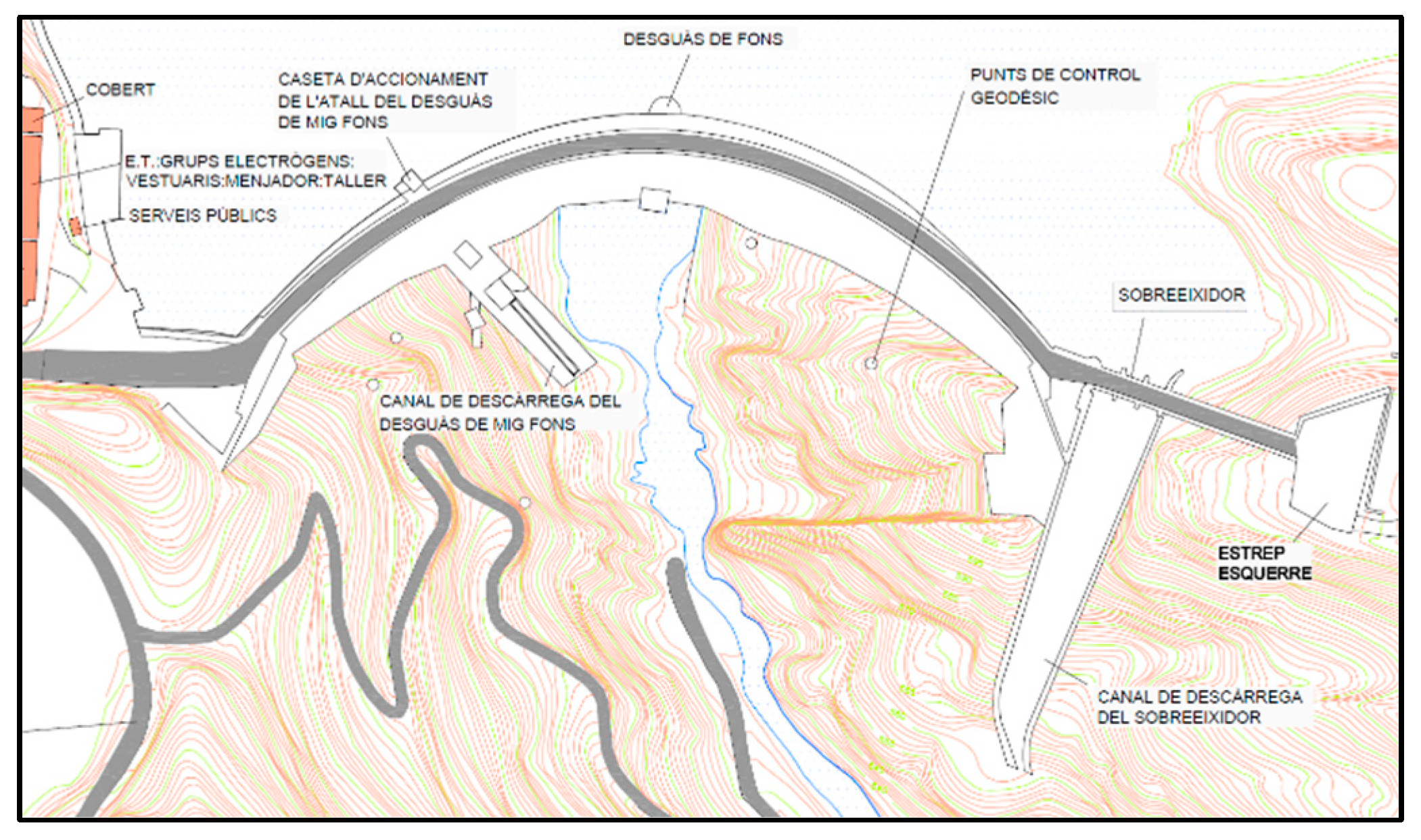
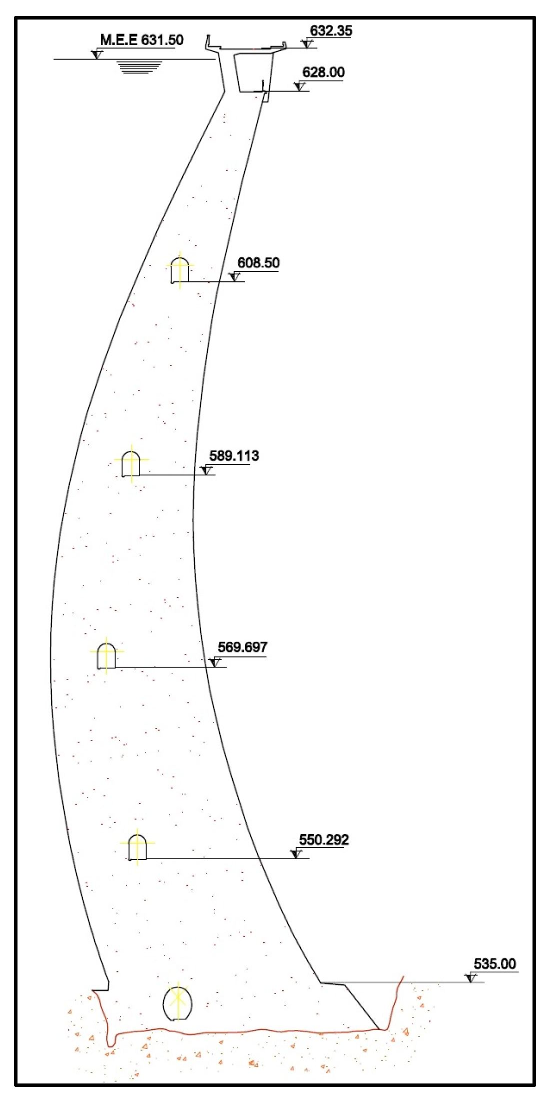
2.4. Study Case

In this study, a concrete arch dam for which real data are available is used as a model. The La Baells dam on the Llobregat river is located in the province of Barcelona (Spain) and closes a reservoir with a total capacity of 109.5 hm³. This dam was built in 1976 with a height of 102.3 m and a crest length of 302.4 m. Its foundation elevation is 530 m and the volume of the dam body is 400,000 m³.

From the existing test campaign, it is considered that the foundation materials are homogeneous and, therefore, there are no different soil strata. The bedrock is composed of a multitude of narrow and almost vertical strata, which can be simplified to mean values of the bedrock properties.

In the first stage, the physical characteristics of the materials (foundation and concrete) are determined in accordance with the values recorded in previous studies conducted at La Baells (

Table 2. Initial properties of materials.

Material	Foundation	Concrete
Density (kg/m3)	3000	2400
Modulus of elasticity (N/m2)	1.962 × 1010	2.452 × 1010
Poisson’s ratio	0.25	0.22

) [21]. In addition, a concrete–concrete friction coefficient for dry conditions of 0.8 is used, following the reports of the Concrete Masonry Handbook [22] and PCI Design Handbook [23].

Geometry

The 3D design is based on the topography records (Figure 2) and the different definition sections of the dam (Figure 3 represents the highest section). The 3D geometry includes the 17 transverse joints, allowing the cantilevers to move independently of each other.

However, soil not immediately adjacent to the dam is simplified, while soil in contact with the dam is included by adapting to the contour lines every five meters in the cartography. In depth, a land area equal to 150% of the height of the dam is included and the lateral extension is equal to 50% of the length of the dam (Figure 4). The characteristics of the mesh are described in Section 4.1.1.

Additionally, the reference reservoir level is set at 620 m above sea level (12.29 m below the crest elevation), reaching 88% of the total height of the dam. In cases where this level is not sufficient, a reservoir level with an overtopping of 5 m above crest elevation is imposed. For simulations where the 5 m overtopping is insufficient, an overtopping of 20 m is applied.

For the study of the effect of cracking, the upstream occurrence of one major crack in the dam is assumed. Lengths and depths of a certain importance are considered to ensure a clearly visible effect on the structure. It was decided to simulate the cracks independently (i.e., they never coexist in the same modeling) since it is not common for several major cracks to coexist in the same dam and the results obtained for such a scenario would be mixed and less understandable.

Only two cracks [24] were simulated since each crack requires considerable computational cost, thus simulating more cracks would require significant increase in computational time with no expected improvement in the accuracy of the results. Upstream cracks of the most common shape and location for arch dams are proposed [24] at those locations since they correspond to the typical locations of cracks in real dams [25]. These are:

-

Horizontal, near the base (Figure 5). This crack has a length of 91.5 m, a depth of 50% of the dam thickness, and is located 9.5 m above the base of the dam.

-

On one side, parallel to bedrock contact (Figure 6). This crack has a length of 60.7 m, a depth of 50% of the thickness of the dam, and begins at 9.5 m above the base elevation of the dam, ending at 38.5 m.

The cracks are treated as fully formed without considering the forming process. The mesh is designed to align the faces of the elements with the faces of the crack. Initially, in the detailed model, the sides of the crack behave according to their real behavior: they can transmit compression and friction and can move independently as long as they do not cross each other. Other alternatives to the interaction of the crack sides are considered in Section 3.2.

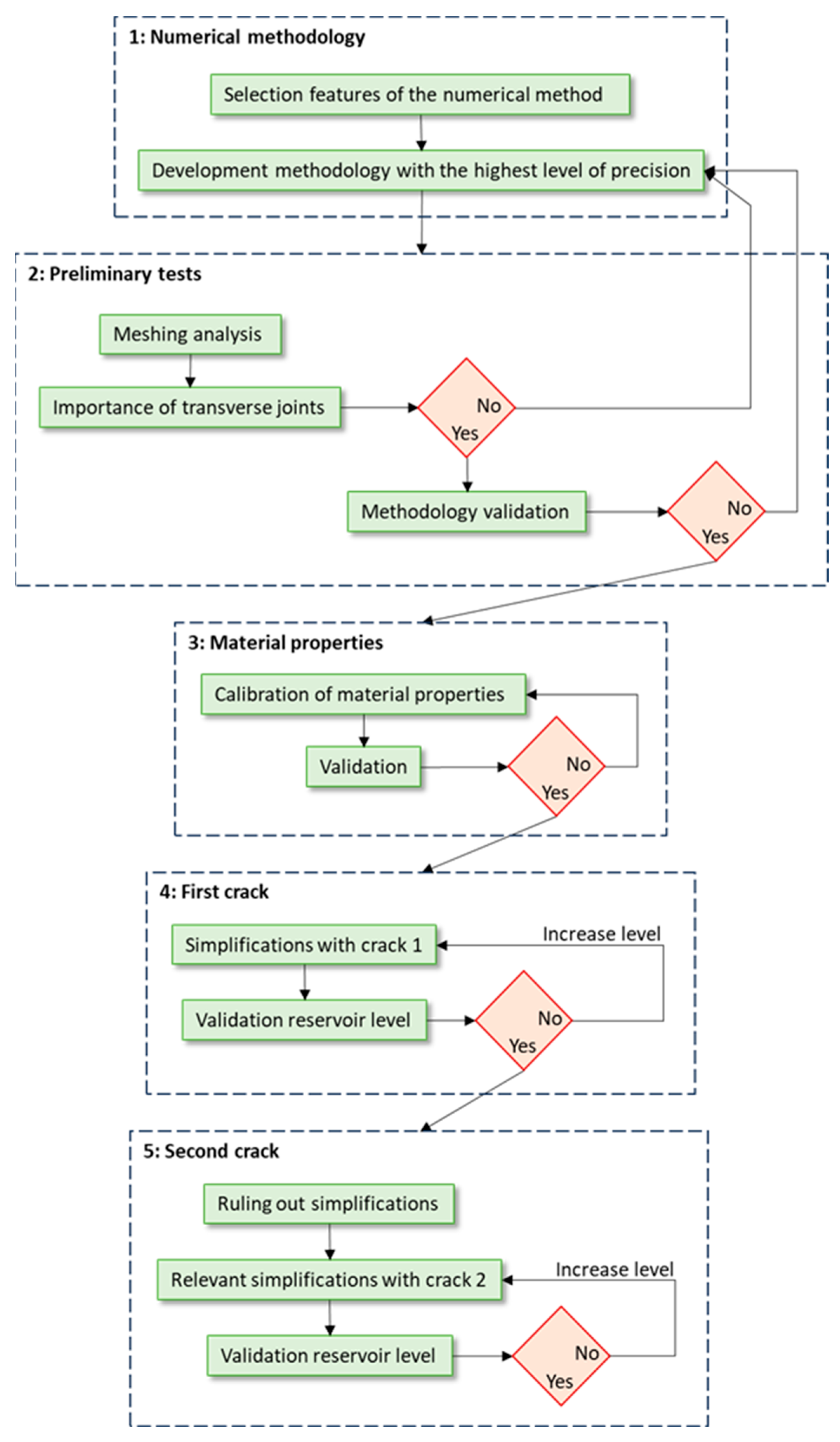
3. Proposed Methodology for Numerical Modeling

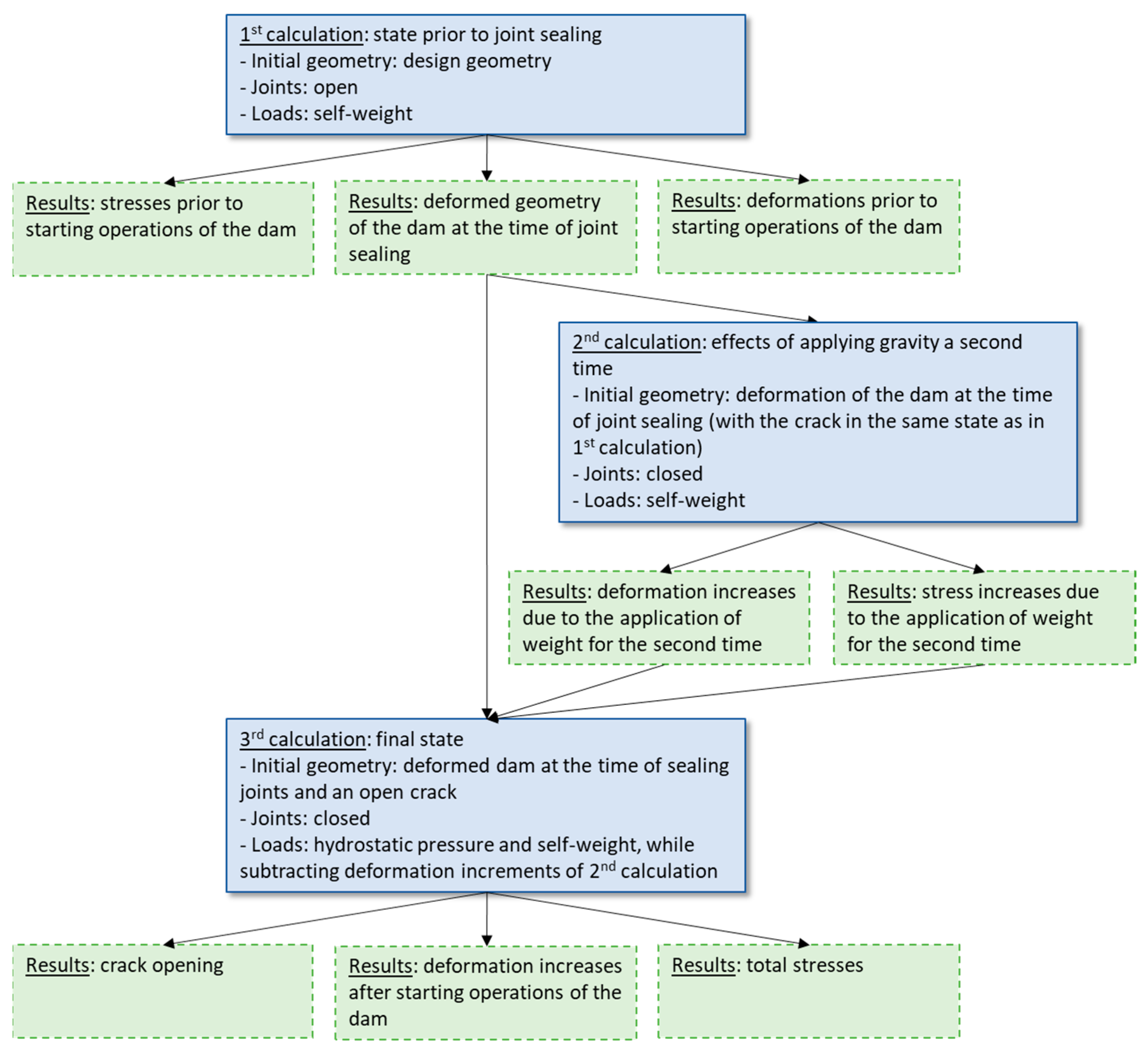
3.1. Base Methodology

As explained in Section 2.2, the only acting forces are due to the self-weight of the dam and the hydrostatic pressure of the reservoir on the upstream face of the dam. The first task of this study is to elaborate a methodology that is as accurate as possible that can be used as a reference to calculate the error of other simpler methodologies. With advanced calculation software, the linear deformations of several solids joined together and subjected to gravity and pressure on one face can be simulated without difficulty. But, to properly consider the real processes that occur in arch dams, including transverse joints, it is necessary to take into account that the dam configuration changes before the hydrostatic pressures occur (but when the self-weight is already acting), with the sealing of transverse joints that turns the different cantilevers into a monolithic solid. And this dam configuration will change again when a crack opens.

In this work, different approaches are tested with different simulation software. The direct approach to this problem is to perform transient simulations, but this involves overcomplicating the calculations (both in complexity and duration). Therefore, an alternative methodology is proposed which, although it is still complex and very precise, is feasible for application. The appropriate simplifications will be made to this methodology, which will be described later, to analyze their effect and determine whether or not they are valid and under what circumstances they can be applied. For the non-transient methodology, an approach based on a succession of stationary calculations combining two very different states was considered:

• Initial calculation with open joints, without any crack and with self-weight being the only load;
• Final calculation on the monolithic dam and with a crack and subjected to hydrostatic pressure.

This approach was not viable due to the impossibility of applying the results of the initial calculation to the final one, since the geometry of the dam differs. A solution was sought by integrating the two calculations into a single process and inserting between them the effect of transforming the cantilevers into a single solid, sealing transverse joints by creating slip-free connections between the cantilevers in their deformed position at the end of the initial calculation.

Lastly, the challenge of allowing gravity to influence the crack faces (which only exist in the final calculation) without duplicating the effect of gravity on the rest of the dam (which is already affected by gravity in the initial calculation) was addressed. To compensate for the effect of gravity affecting the model twice, an intermediate calculation is performed to obtain the deformations and stresses due to gravity in the entire dam excluding the sides of the crack and then they are subtracted from the final calculation (Figure 7). In models with a crack that can open, the deformations that are subtracted in the 3rd calculation are not the same as those caused by gravity in the 3rd calculation (apart from the case of simplification C in Section 3.2). The difference between these two deformations corresponds precisely to the effect of gravity on the crack.

Finally, it should be clarified that this three-step methodology is only necessary because of the inclusion of a crack that is affected by gravity after the joint sealing (while the rest of the dam is affected before the joint sealing). In a case that does not include cracking, this intermediate calculation would not be necessary.

3.2. Methodology Simplifications

After establishing the most accurate resolution methodology, different simulations are proposed to check the error they produce by studying how the results vary when these simplifications are introduced in the model.

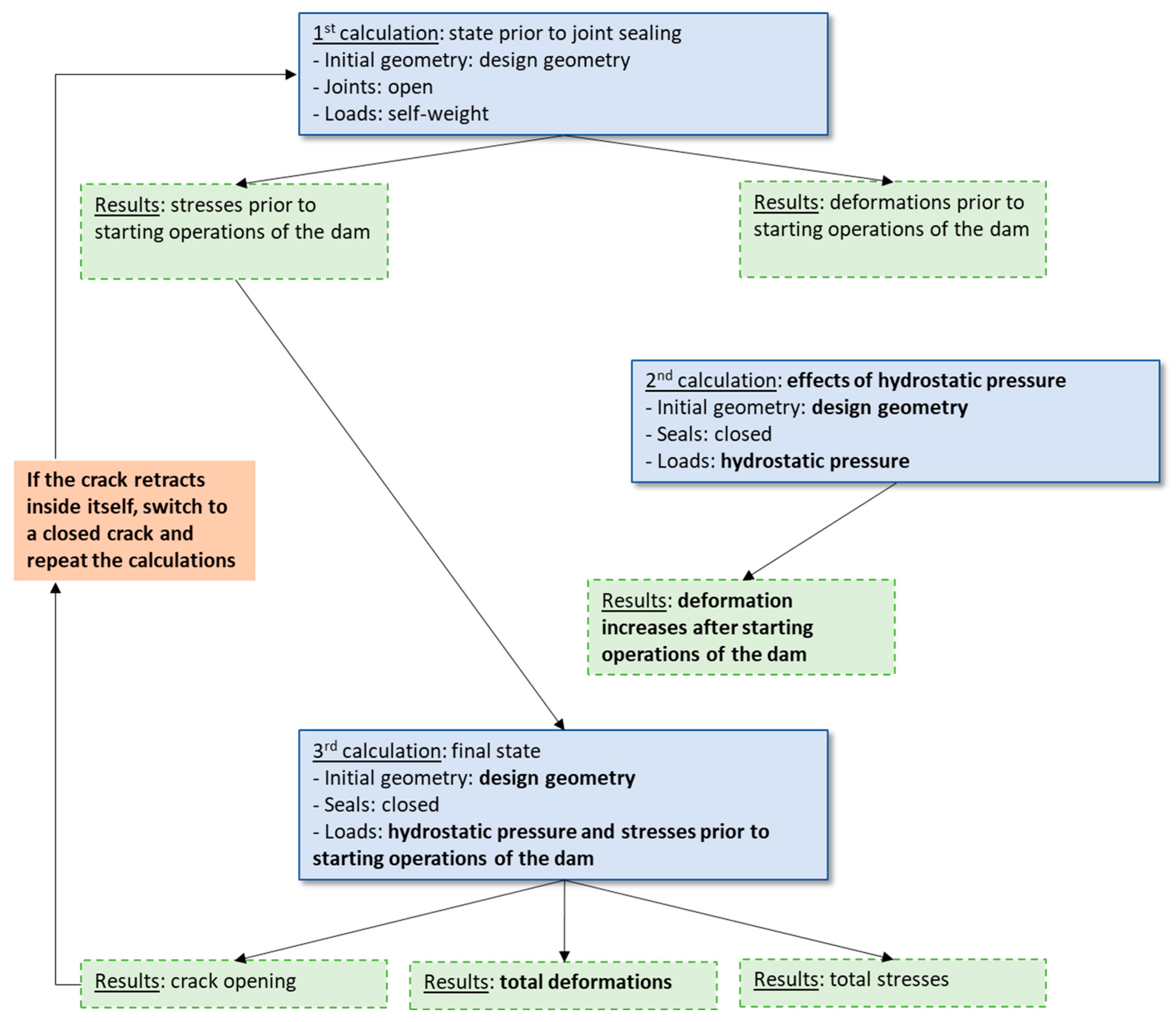
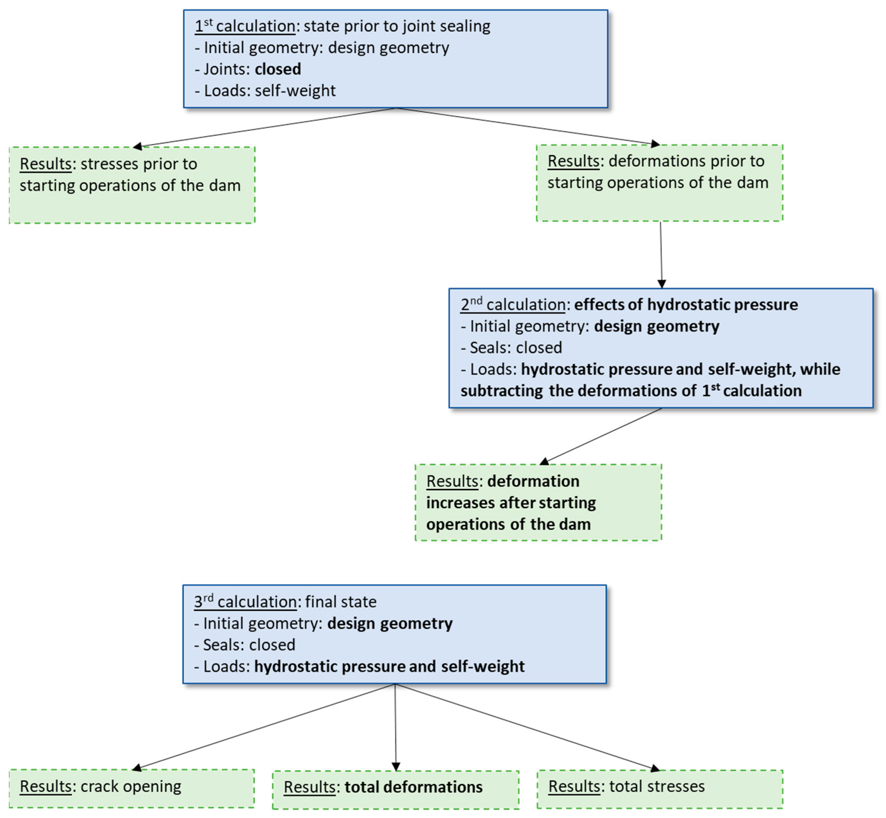
• Simplification A: the transverse joints are closed before self-weight is applied. In this way the cantilevers can never deform independently of each other. The methodology still consists of a first phase before starting operations where only self-weight is applied and a second phase beginning with the deformed geometry of the previous phase where hydrostatic pressure and a crack are applied.
• Simplification B: the crack already exists at the beginning of the simulation. In this case the self-weight is applied on an already-cracked dam.
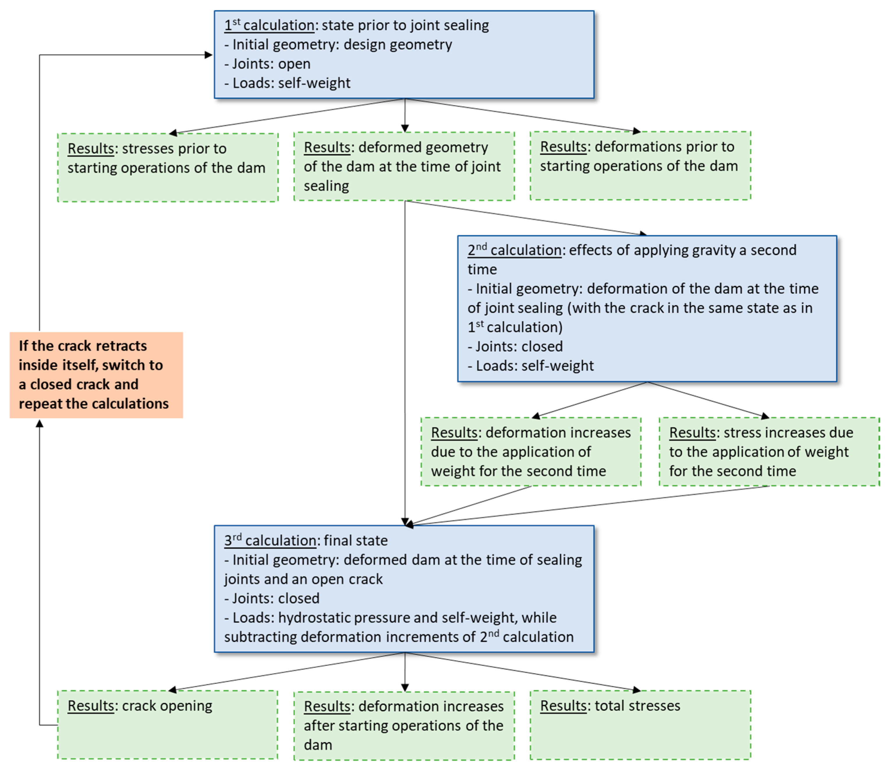
• Simplification C: the crack faces are disconnected, allowing the upper side of the crack to pass through the lower side in its movement. Therefore, the crack faces can either separate (open crack) or ride over each other (with a non-existent penetration, which in reality corresponds to a closed crack). In these simplifications, if the final result indicates that the sides of the crack cross each other, it is necessary to repeat the simulation, establishing that the joint cannot open, as shown in the scheme of Figure 8. As already discussed in Section 3.1, the deformations that are subtracted in the 3rd calculation are not equal to those caused by gravity in the 3rd calculation. There is an exception when the crack can close on itself in the first calculation and another exception when the crack is not free to open in any of the calculations (this happens in simplification C where the calculation is repeated, i.e., when the hydrostatic pressure is not sufficient to open the crack).

In the next step, the three simplifications discussed above are combined in the cases indicated in Figure 9.

Simplification 2, although a conceptually simpler approach, does not reduce the calculations with the software being used. This software performs two simulations: one with open joints and then another with sealed joints in the final position of the first simulation. By solving two separate simulations there is no numerical advantage of considering the crack in the same state in both parts of the calculation. However, it has been proposed because with other FEM packages it can be an advantageous simplification.

On the other hand, it can be noted that applying the proposed methodology to simplification 5 results in an incorrect physical approach since the joints would be sealed when the crack is crossing itself due to its own weight, but in the final stage of the calculation, the hydrostatic pressure has no freedom of movement to compensate for these deformations in the joint plane.

Since simplification 5 is not feasible with this methodology, we propose an alternative methodology which we call simplification 5.1 (explained in Figure 10). This consists of calculating separately the stresses for self-weight and then applying them to another simulation with hydrostatic pressure. In the self-weight design, the joints are open and the cantilevers can penetrate each other, while in the hydrostatic pressure design the joints are closed.

Additionally, two alternative methodologies, called simplifications 4.1 and 7.1 (explained in Figure 11 and Figure 12), are also included. In these simplifications, the hydrostatic pressure calculation is performed on the base geometry and not on the deformed geometry resulting from self-weight. These alternatives are studied because it is common practice to perform all calculations on the original geometry. These alternative versions only apply to simplifications 4 and 7, because only in these simplifications do both the joints and the crack function in the same way before and after sealing the joints. Thereafter all the simplifications of the study are summarized in Figure 13.

4. Results and Discussion

4.1. Preliminary Tests

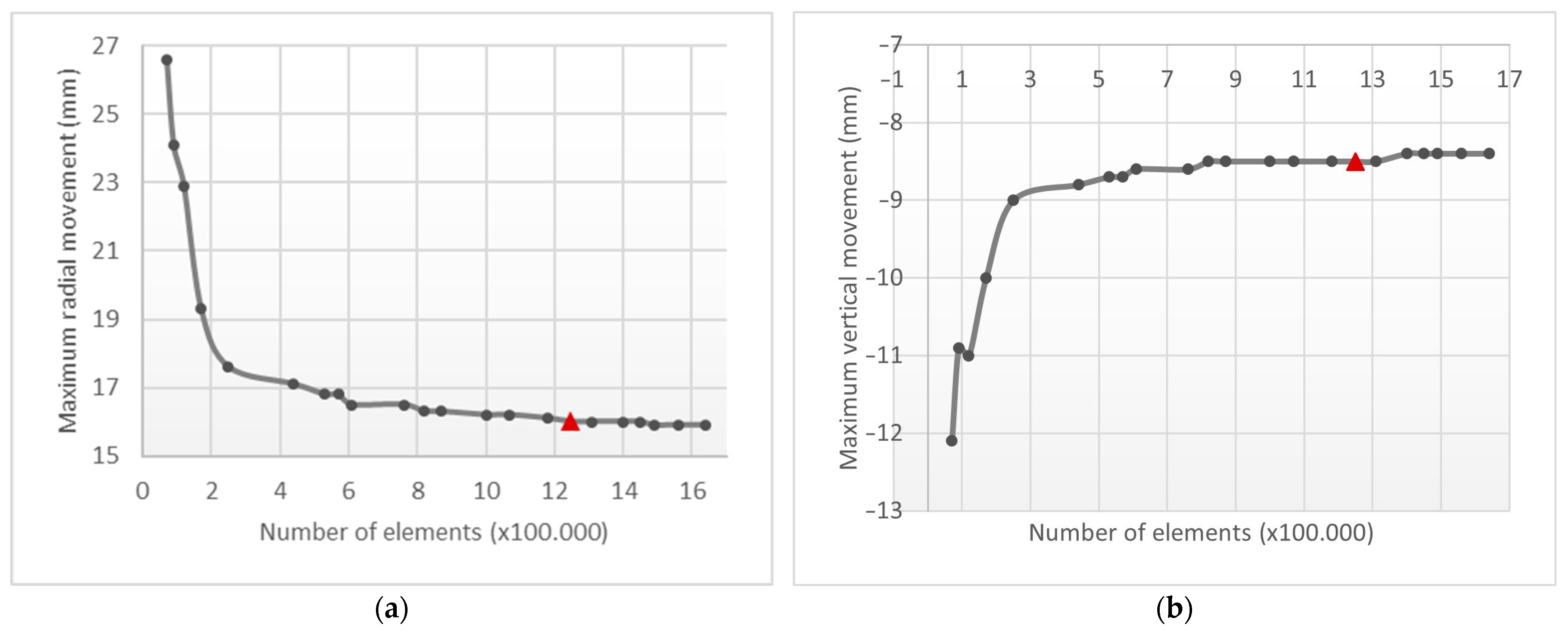
4.1.1. Mesh Analysis

In this part of the study, a procedure is performed for the selection of the most suitable mesh size through simulations with different mesh sizes, comparing the variation in the results. The meshes used are formed by tetrahedrons with a quadratic element order and a growth ratio of 1.1. The rest of the parameters have been established to maintain a compromise between the calculation time and quality of the result. The characteristics of each mesh are described in

Table 3. Characteristics of fine meshes (* bedrock elements are 10 times larger than indicated).

Element Size * (m)	1.00	1.02	1.04	1.05	1.07	1.10	1.12	1.15	1.20	1.235	1.319
Number of nodes × 10−5	25.0	23.7	22.7	22.2	21.3	20.0	19.2	18.0	16.5	15.4	13.3
Number of elements × 10−5	16.4	15.6	14.9	14.5	14.0	13.1	12.5	11.8	10.7	10.0	8.7

and

Table 4. Characteristics of large meshes (* bedrock elements are 10 times larger than indicated).

Element Size * (m)	1.35	1.40	1.55	1.60	1.65	1.80	2.40	3.00	3.60	4.20	4.80
Number of nodes × 10−5	12.6	11.7	9.4	8.8	8.2	6.9	3.8	2.6	1.9	1.4	1.1
Number of elements × 10−5	8.2	7.6	6.1	5.7	5.3	4.4	2.5	1.7	1.2	0.9	0.7

; some examples are shown in Figure 14.

The maximum displacement results are considered to be stabilized when the variation upon mesh refinement is equal to or less than the measurement error of the monitoring devices (0.1 mm). As can be appreciated in Figure 15, this is achieved with a mesh size of 1.15 m (1,180,000 elements).

In the next step, comparisons of computation time according to mesh size are conducted, using as reference the one-million-element mesh in Table 3. It can be observed in Figure 16a that the computation time oscillates widely, although by tracing a trend line (dashed line) it is possible to estimate the increase in computation time with respect to the mesh size. The reference time used is for a one-million-element model.

The oscillation of the calculation time Is due to the fact that the calculation of the phase with open transverse joints (which corresponds to most of the calculation time) is iterative and the number of iterations is not proportional to the mesh size, as can be seen in Figure 16b.

The following phase studies the calculation time per iteration taking into account only the part of the calculation with open joints (Figure 17) so that the increase in calculation time when changing the mesh size can be seen more clearly.

Figure 18 shows the situation of the transverse joints. Initially, in the self-weight phase of the detailed model, the sides of the joints behave according to their real behavior: they can transmit compression and friction and can move independently as long as they do not cross over each other. While in the hydraulic loading phase they behave monolithically: the sides of the same joint deform jointly, always maintaining the same relative position they had at the end of the self-weight phase. Other alternatives to the interaction of the crack sides are considered in Section 3.2.

4.1.2. Importance of Considering Open Joints

To study the relevance of discarding the effect of the transverse joints, a simulation of deformations due to self-weight was carried out with open joints and another with closed joints. Figure 19 and Figure 20 show the differences between the displacements obtained with these two solutions. It can be seen in the images how the maximum radial movements drop from 20 mm to 5 mm and the vertical movements from 11 mm to 8 mm.

Furthermore, on analysis of the variation in circumferential stresses in the upstream face, it is noted that in most of the dam the error is below 0.2 MPa, increasing at the base to values greater than 1 MPa. On the other hand, in the vertical stresses, the error is generally lower than 1 MPa, increasing at the base up to values higher than 5 MPa. It should be mentioned here that the stress values obtained by FEM models in the contact zones between materials with different stiffnesses (dam–bedrock) usually present high gradients, due to the mathematical formulation itself, so the difference in the results in this zone between different approximations was to be expected.

Due to the values of these differences and those of the displacements, it was decided to include transverse joints as part of this study.

4.1.3. Validation of the Proposed Methodology

In order to validate that the intermediate-step approach provides consistent results, a simulation with a zero reservoir level was performed. It was expected that in this simulation the increase in the deformation after starting operations (injection of joints) would be zero. Figure 21 and Figure 22 show the differences in radial and vertical displacements. The results obtained are not completely zero due to the intrinsic inaccuracy of the numerical calculation, but the variation can be considered negligible, with maxima of 0.13 mm in radial movement, 0.08 mm in circumferential, and 0.18 mm in vertical.

The next step involves a comparative analysis of the final stresses, for which it is convenient to divide the dam into two zones: one zone comprises the area around the upstream dam–bedrock contact while the other zone contains all the remaining areas of the dam.

• In the remaining areas of the dam, it was found that, assuming an empty reservoir level, the resulting total stresses are equivalent to those obtained in the first calculation. Again, the variation is not zero due to the inherent inaccuracy of the numerical calculation.
• In the area around the upstream dam–bedrock contact, the discrepancies between the results of the methodology and one-step numerical calculation are not negligible. This zone corresponds to an area of high stresses and a geometry with a large number of corners. As a result, this leads to fictitious stress increases due to the resolution of numerical models (which applies to any FEM technique), even though in reality there would be a smoother stress distribution in this area. In the absence of reference values, it becomes unclear whether the error made by the proposed methodology would be significantly greater than the error made by the direct numerical computation. It should be noted that this particularity of the results applies to stresses and not to movements (due to the mathematical formulation of the FEM).

Therefore, the variation in the body of the dam can be considered negligible since the differences in vertical stresses are less than 0.1 MPa. From the above tests, it can be safely accepted that the numerical simulation methodology proposed in this study will be suitable for the calculation of displacements in the whole dam and for the calculation of stresses in the parts of the dam that are not close to the bedrock.

4.2. Calibration Tests

In order to assess the influence that the variation in material property values, due to their uncertainty, can have on the displacements of the model, it was measured the differences resulting from the application of low and high extreme values of the material properties. These values are defined according to Hariri-Ardebili [26], i.e., distanced from the initial value twice the standard deviation with a coefficient of variation of 0.15 and using the design data as the mean value (

Table 5. Variability in material properties.

Parameter	Low	Design	High	Units
Density (Concrete)	2100	2400	2600	kg/m3
Poisson’s Ratio (Concrete)	0.154	0.22	0.286	-
Poisson’s Ratio (Soil)	0.175	0.25	0.325	-
Young’s Modulus (Concrete)	17,164	24,520	31,876	MPa
Young’s Modulus (Soil)	13,734	19,620	25,506	MPa

) with a correction to the density values by adjusting them to the limits for the concrete of a dam.

In

Table 6. Error in maximum displacement results.

	Max. Radial Displacement		Max. Vertical Displacement
Parameter	Low	High	Low	High
Density (Concrete)	−0.2%	0.2%	−0.1%	0.3%
Poisson’s Ratio (Concrete)	0.8%	−0.9%	1.4%	−2.1%
Poisson’s Ratio (Soil)	0.3%	−0.2%	−0.5%	0.8%
Young’s Modulus (Concrete)	−34.6%	18.6%	−32.3%	17.7%
Young’s Modulus (Soil)	−8.4%	4.4%	−9.9%	5.7%

, it is seen that even when implementing extreme variations, the only parameter that causes a variation greater than 2.1% is the Young’s modulus (this conclusion agrees with the results of other studies [20]). According to these results, it is decided to calibrate the model for Young’s modulus, using the mean design values for the rest of the parameters.

The centroid method is used for calibration by means of the movements in the central cantilevers [27]. Starting from the design values several higher levels are included, following the same ranges as in Table 5. The 18 pairs of Young’s moduli that result from combining these values constitute the exploration points.

Afterwards, simulations corresponding to the 18 cases are performed and their errors for each case are determined (

Table 7. Global relative error in radial displacement results.

			Concrete (MPa)
		24,520	31,876	39,232
Soil (MPa)	19,620	0.96454459	0.09823328	0.02290233
	25,506	0.75630712	0.04730953	0.06258044
	31,392	0.63728901	0.02915880	0.10764353
	37,278	0.56073436	0.02344675	0.14367899
	43,164	0.50762649	0.02283556	0.17308593
	49,050	0.46889552	0.02448376	0.19845217

).

In the next step, a maximum permissible error is stipulated (set in 0.023) which serves to delimit the solution domain. The coordinates of points on the solution domain contour are calculated by linear interpolation of the errors previously obtained (

Table 8. Coordinates of the solution domain contour.

			Concrete (MPa)
		31,873.5	31,876.0	31,884.1
Soil (MPa)	41,580.4		0.0230
	43,164.0	0.0230	0.02283556	0.0230
	43,751.2		0.0230

).

Finally, the centroid of the solution domain is found from these contour points, obtaining the values concrete: 31,877.02 MPa; and soil: 42,831.87 MPa.

The error is tested by solving a numerical simulation with these values (

Table 9. Errors for each radial displacement obtained with calibrated Young’s moduli.

	Cantilever 2-I		Cantilever 1-D
P0 measurement	−0.60 mm	4.93%	−0.94 mm	8.0%
P1 measurement	0.04 mm	−0.4%	−0.52 mm	5.6%
P2 measurement	0.69 mm	−10.5%	0.08 mm	−1.3%

) proving that it corresponds to an allowable value.

Once the updated value of the modulus of elasticity is obtained, the method is validated by measuring the error (

Table 10. Validation based on the errors in each radial displacement result.

	Cantilever 2-I		Cantilever 1-D
P0 measurement	0.04 mm	0.4%	1.00 mm	13.9%
P1 measurement	−0.66 mm	−10.1%	0.12 mm	2.1%
P2 measurement	−1.21 mm	−27.5%	−0.80 mm	−20.1%

and Figure 23) with the other pair of dates in Table 1.

Therefore, the calculations show that this methodology provides deformations in an order of magnitude equivalent to those measured by the apparatus. Thus, it allows a study to be performed on the effects of a synthetic crack on the displacements of an arch dam.

4.3. Accuracy for Different Simplifications: Crack 1

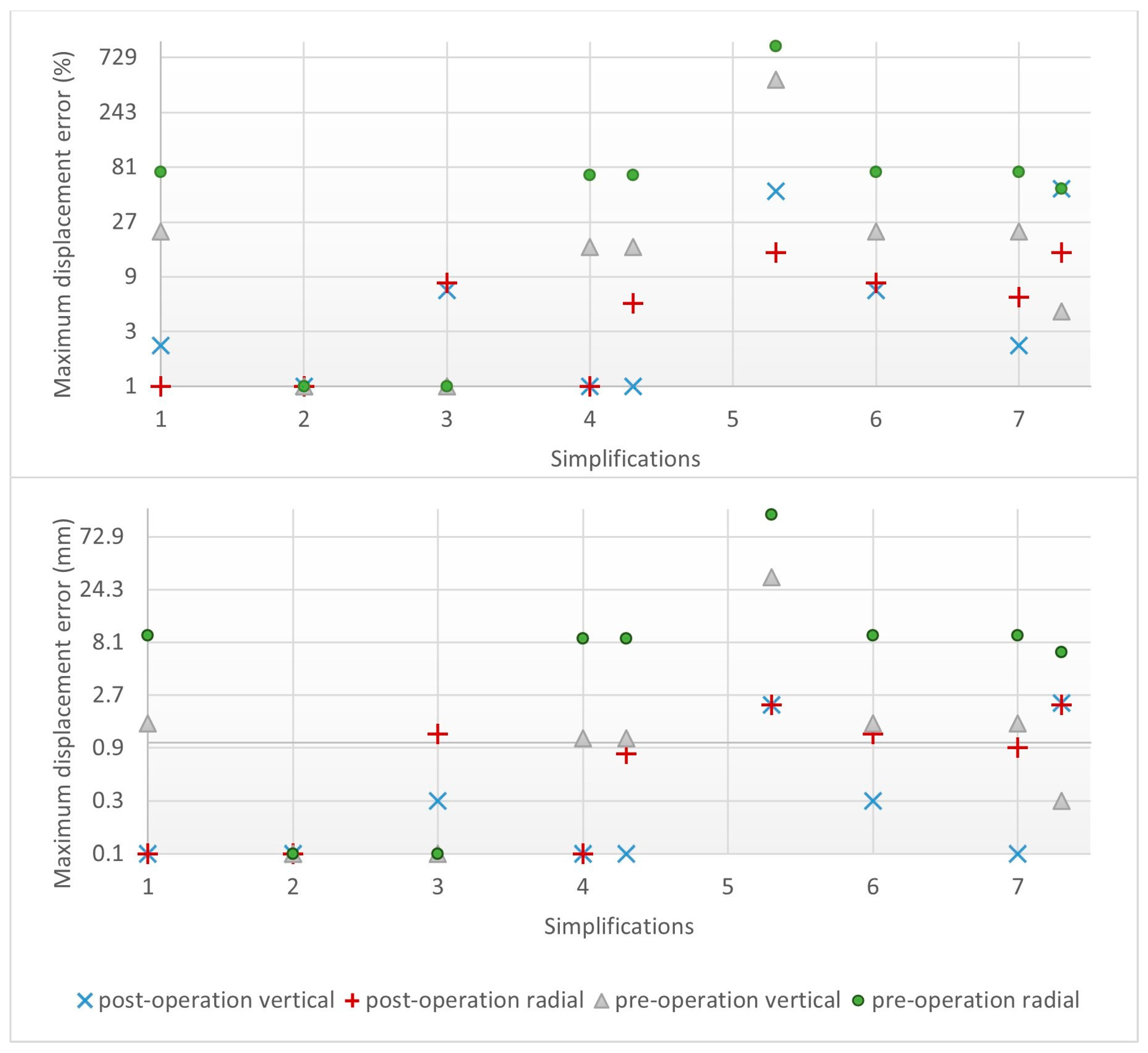
4.3.1. Absolute and Relative Displacement Errors

Figure 24 shows the errors in relation to the maximum values of displacements measured on a logarithmic vertical scale.

Noteworthy in these figures are the values before starting operations for simplification 5.1 because they exhibit values on a significantly larger scale than the rest of the measured simplifications. These large errors are due to the fact that the cantilevers can penetrate through each other.

Simplifications 1, 4, 4.1, 6, 7, and 7.1 also show distinctly deviating results before starting operations (gray triangle and green circle) due to the fact that the joints are sealed. Considering the coordinates of the point where these displacements occur, it can be seen that these simplifications also obtain a very different location in the calculation prior to starting operations.

At first sight, it can be seen in the results of displacements after application of the hydraulic pressure (red cross and blue X) that simplifications 3, 6, 5.1, 7, and 7.1 produce results with larger errors; this is assumed to be because there is no friction between the crack faces and no stresses are transmitted.

The results show that the crack opening with the chosen reservoir level is only 0.1 mm. For a better verification of the effect of the simplifications regarding the crack opening, the calculations are repeated, but this time applying a fictitious overtopping of 5 m above the crest elevation. Figure 25 shows the errors in relation to the maximum displacement values.

In the same way as with the previous reservoir level, simplifications 1, 4, 4.1, 6, 7, and 7.1 produce very different results, including coordinates, before starting operations (gray triangle and green circle) as the joints are sealed. Simplifications 3, 5.1, 6, 7, and 7.1 also produce results with larger errors in the displacement results after applying the hydraulic pressure (red cross and blue X) because there is no friction between the crack faces and no stresses are transmitted.

In this figure, the values before starting operations for simplification 5.1 stand out because they are outside the range of the rest of the values. These significant errors are due to the fact that the crack closes on itself, which is then compensated by the hydraulic pressures for the final results.

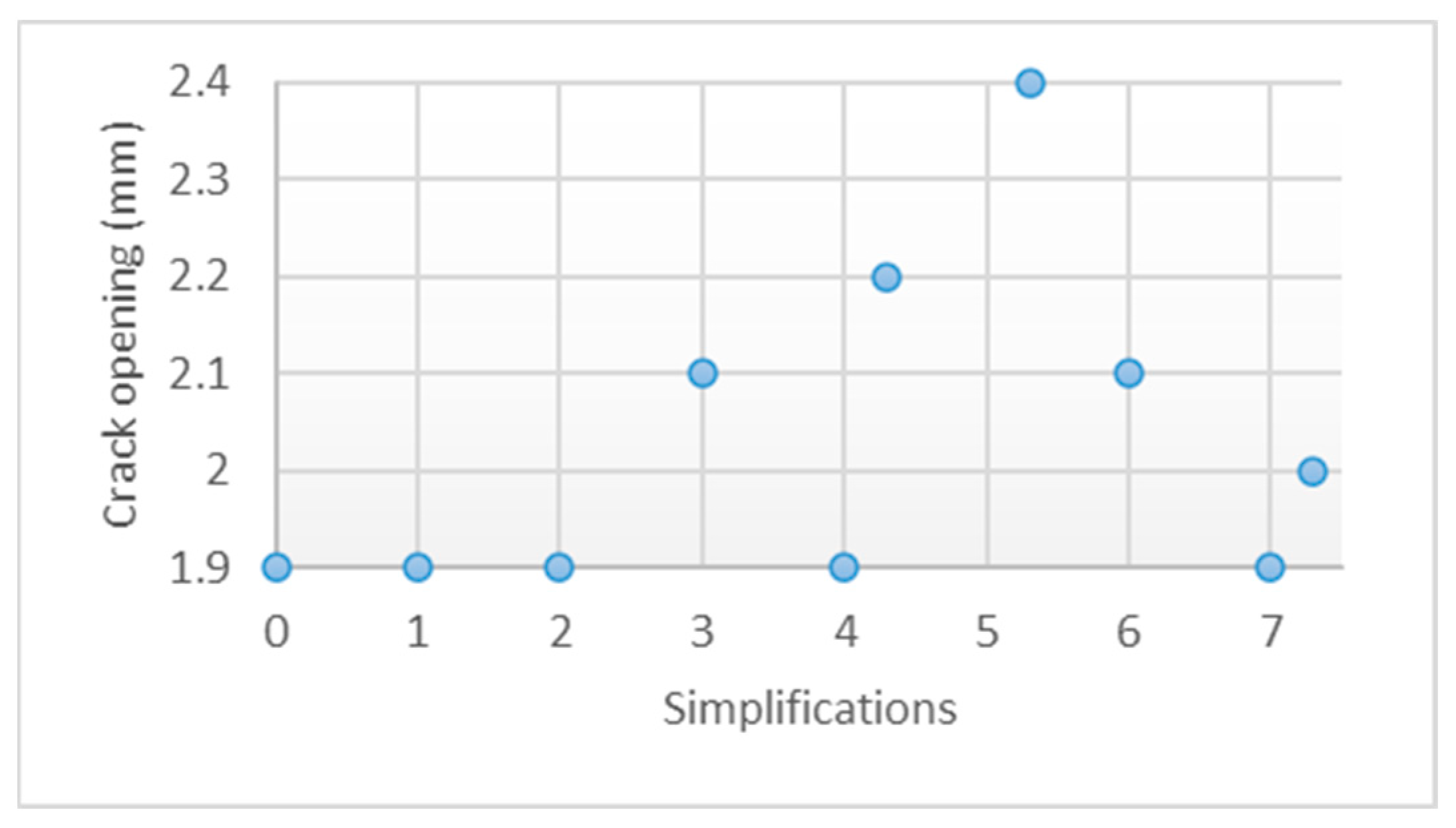
4.3.2. Crack Opening

Additionally, in this second set of comparisons, the maximum crack opening at the end of the simulation is included (Figure 26). It can be seen that the simulations where there is no transmission of forces between the sides of the crack (simplifications 3, 6, 5.1, 7, and 7.1) tend to overestimate the crack opening.

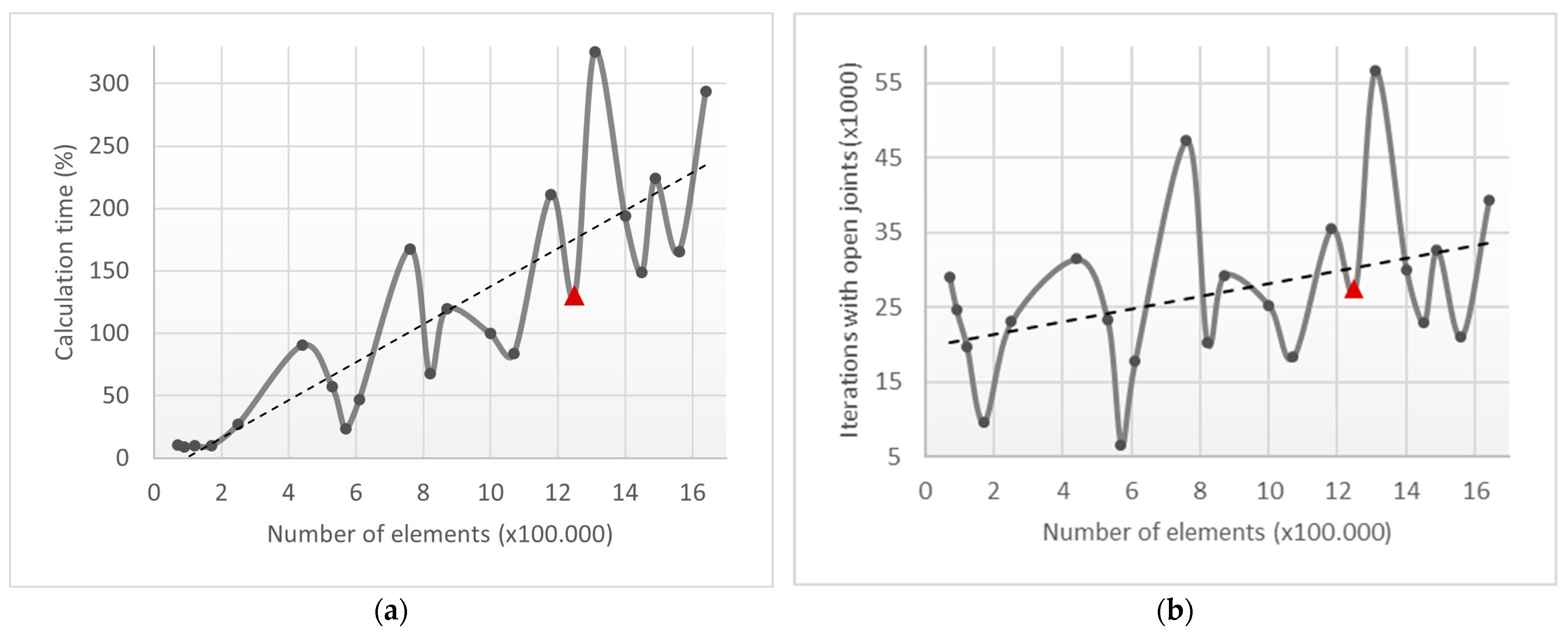
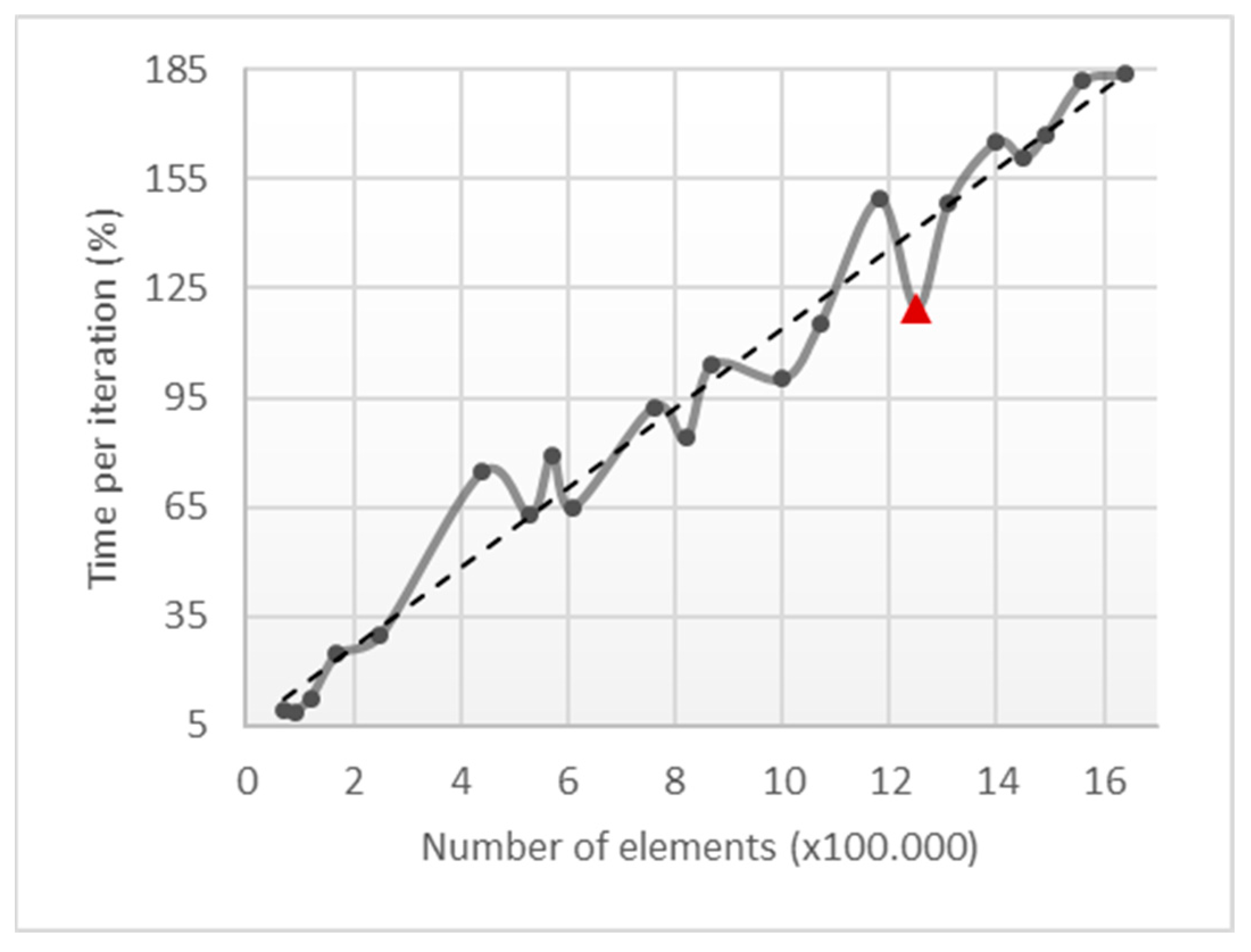
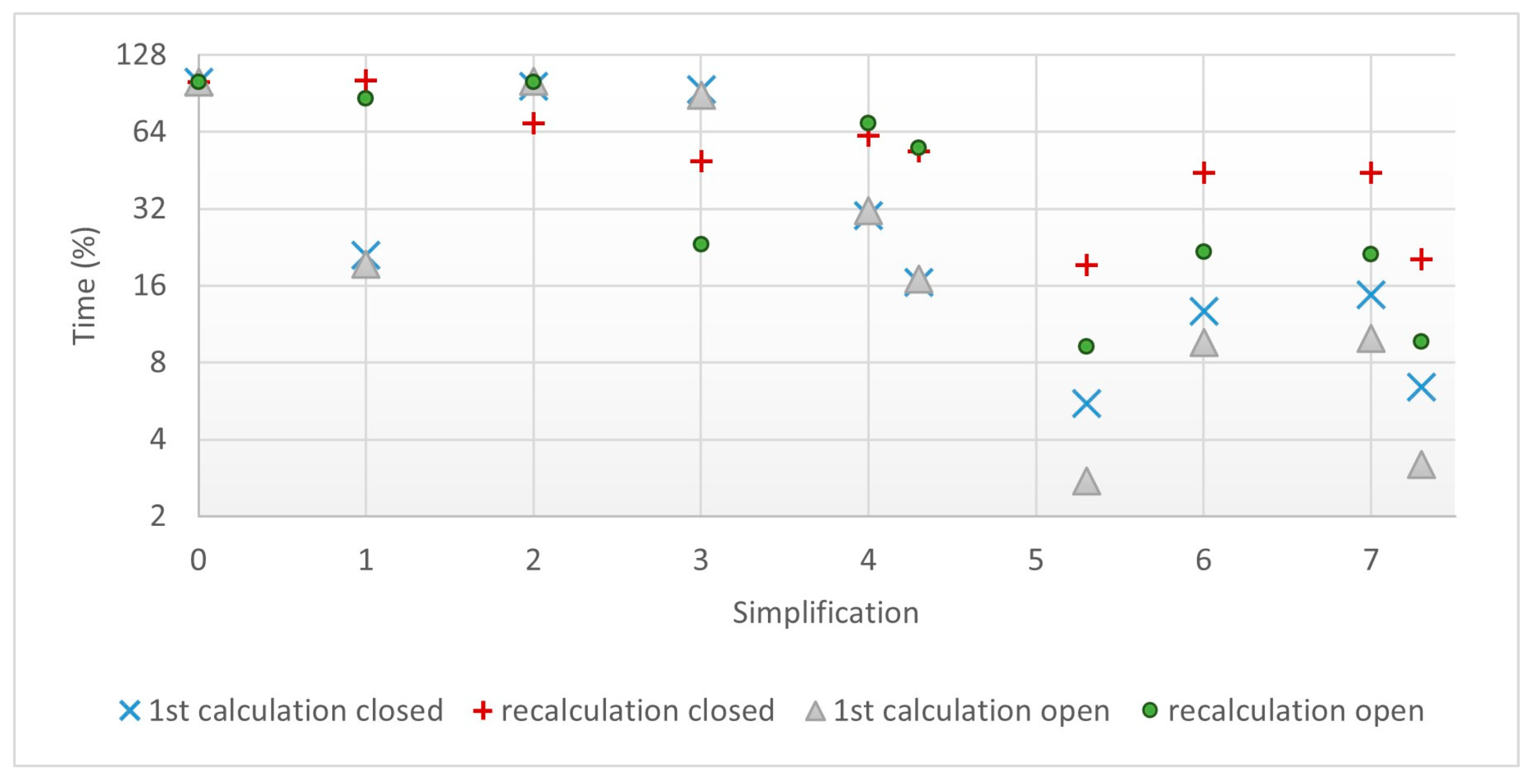
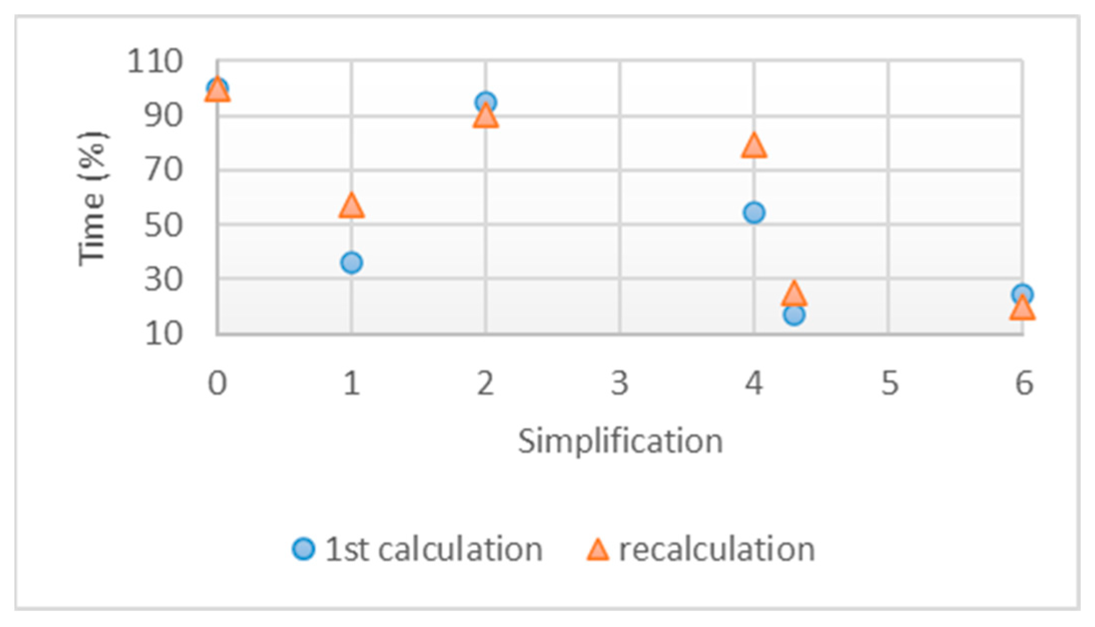
4.3.3. Calculation Time

Figure 27 compares the calculation times of the different simplifications, both those that result in an open crack and those that do not. Two phases are compared, first the time of a complete simulation with a given reservoir level, and subsequently the time to recalculate the same simulation modifying only the reservoir level.

At first sight, it can be observed that all simplifications reduce the computation time, and this reduction is greater when two simplifications are combined. It can be seen how in the cases where the sides of the crack cannot penetrate each other (accurate and simplifications 1, 2, 4, and 4.1), it takes the same calculation time when the crack is opened as when it is not.

From the results shown, it can be concluded that simplification 2 is the only one that gives results equivalent to the most accurate approach in all cases. Analyzing the results before applying the hydraulic pressure, simplification 3 also offers results without error, this is due to the fact that it is the only one that does not apply any change prior to the hydraulic load.

Considering only displacements occurring after the first filling of the dam, simplifications 1, 2, and 4 (the hydraulic pressure is applied on the deformed geometry and the crack cannot close on itself) produce the best results. The errors are 2% or less.

Based on these results, simplifications 5.1 and 7.1 are discarded because their results lead to errors greater than 28% in both the pre- and post-starting operations calculations and at both the overtopped and the initial reservoir level. Simplification 7 is also discarded for the same reason because, although it only obtains errors of 6% in the calculations after commissioning with the initial reservoir level, this is only because when the crack closed on itself the corrective procedure of methodology 7 was applied, eliminating the crack. This means that methodology 7 only works acceptably when it is not applied as a whole.

Finally, simplification 3 is discarded because it does not involve changes regarding the calculation prior to the hydrostatic pressure, it does not offer good results in the posterior calculations and its calculation time is the same as for the first calculation.

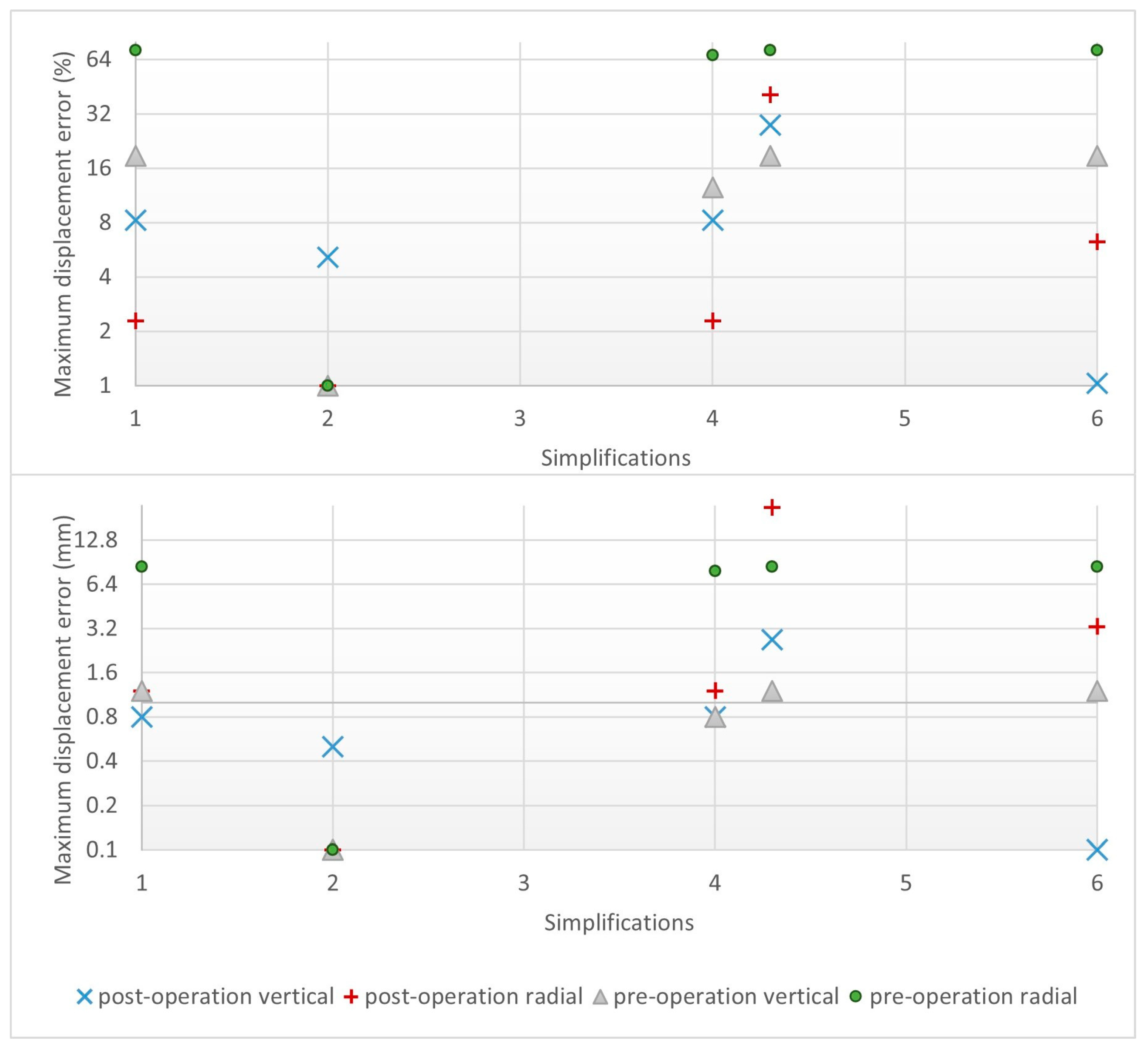
4.4. Accuracy for Different Simplifications: Crack 2

Subsequently, in the next phase of the study, only the most relevant simplifications (1, 2, 4, 4.1, and 6) are compared using the second crack. It is decided to solve only the case involving an overtop because it is more informative. The results reveal that the 5 m overtop is insufficient to open the crack, so a 20 m overtop is simulated (Figure 28 and Figure 29).

Similar to the first crack, simplifications 1, 4, 4.1, and 6 produce significantly different results before starting operations (gray triangle and green circle) because the joints are sealed. Considering the coordinates of the point where these displacements occur, it can be seen that these simplifications also obtain a very different location in the calculation prior to starting operations. In case 4.1, a substantial error also appears in the values of the largest displacements after starting operations.

It can be noted that simplification 6 (where the crack faces do not transmit stresses or friction) overestimates the crack opening.

In addition, Figure 30 compares the calculation times of the different simplifications.

Lastly, Figure 31 summarizes the final results obtained. For each simplification, the decrease in calculation time for each of the cases studied (average of crack 1 with overtop and crack 2 with overtop) is indicated horizontally. The vertical axis shows, for each of these calculations, the errors in the results after starting operations: the maximum vertical displacement, the maximum horizontal displacement, and the crack opening.

5. Conclusions

From the results shown, it can be concluded that simplification 2 is the one that gives results more equivalent to the precise approach in all cases. This is due to the fact that the only change in this simplification is that the crack already exists prior to the application of hydraulic pressure, at which time there are only compressive forces, so there is no appreciable variation in the results.

5.1. Before Hydraulic Pressure

Considering only displacements occurring before the hydraulic loading of the dam, all simplifications show errors greater than 50% with the exception of simplifications 2 and 3. However, simplification 3 was rejected since it does not involve changes regarding the calculation prior to the hydrostatic pressure and does not offer good results afterwards.

5.2. After Hydraulic Pressure

Considering only displacements occurring after the first hydraulic loading of the dam (Figure 31), simplifications 1, 2, and 4 (the joints are sealed before the self-weight is applied and the crack cannot close on itself) produce the best results, showing errors of less than 1.3 mm.

Table 11. Conclusions after first hydraulic loading.

	Description	Average Reduction in Calculation Time	Error in Maximum Vertical Movements	Error in Maximum Radial Movements	Recommendation for Use
Complete approach	The most accurate approach	-	-	-	Single or low number of calculations
Simplification 6	Transverse joints are closed before self-weight is applied and crack sides can pass through themselves	−83%	4.0% 1/1.0% 2	6.5% 1/6.3% 2	Large number of calculations with changes in the geometry or crack locations
Simplification 1	Transverse joints are closed before self-weight is applied	−72%	1.1% 1/8.3% 2	0.6% 1/2.3% 2	Low number of calculations with changes in the geometry or crack locations

¹ First crack. ² Second crack.

shows the two simplifications with the best results in terms of reduction in computational time and errors in maximum displacements (vertical and radial). The errors for crack 1 and crack 2 are shown separately. Finally, some general recommendations are as follows:

• If a single calculation is to be performed, the recommendation is to use the complete (accurate) approach. Since the difference in calculation time between the fastest and slowest simulation is an acceptable time for a single simulation.
• If several calculations are to be performed by varying only the loads after the application of the hydraulic pressure, it is also recommended to use the complete (accurate) approach. The difference in calculation time between the fastest and the slowest simulation remains an acceptable time for a study.
• If many calculations are to be made by changing the loads prior to starting operations or the geometry (including cracks), it may be convenient to use simplification 1 or 2, depending on the availability of calculation time and the required accuracy.

References

1. Li, Z. Global Sensitivity Analysis of the Static Performance of Concrete Gravity Dam from the Viewpoint of Structural Health Monitoring. Arch. Comput. Methods Eng. 2021, 28, 1611–1646. [Google Scholar] [CrossRef]
2. ICOLD World Register of Dams. General Synthesis. Number of Dams by Country Members. Available online: https://www.icold-cigb.org/article/GB/world_register/general_synthesis/number-of-dams-by-country (accessed on 29 February 2024).
3. ICOLD/CIGB. Constitution Statuts; ICOLD/CIGB: Paris, France, 2011. [Google Scholar]
4. Hariri-Ardebili, M.A.; Saouma, V.E. Seismic Fragility Analysis of Concrete Dams: A State-of-the-Art Review. Eng. Struct. 2016, 128, 374–399. [Google Scholar] [CrossRef]
5. Gharibdoust, A.; Aldemir, A.; Binici, B. Seismic Behaviour of Roller Compacted Concrete Dams under Different Base Treatments. Struct. Infrastruct. Eng. 2020, 16, 355–366. [Google Scholar] [CrossRef]
6. ASCE. Report Card for America’s Infrastructure; ASCE: Reston, VA, USA, 2021. [Google Scholar]
7. Hariri-Ardebili, M.A. MCS-Based Response Surface Metamodels and Optimal Design of Experiments for Gravity Dams. Struct. Infrastruct. Eng. 2018, 14, 1641–1663. [Google Scholar] [CrossRef]
8. Oliveira, S.; Faria, R. Numerical Simulation of Collapse Scenarios in Reduced Scale Tests of Arch Dams. Eng. Struct. 2006, 28, 1430–1439. [Google Scholar] [CrossRef]
9. Zheng, D.; Huo, Z.; Li, B. Arch-Dam Crack Deformation Monitoring Hybrid Model Based on XFEM. Sci. China Technol. Sci. 2011, 54, 2611–2617. [Google Scholar] [CrossRef]
10. Wang, W.; Ding, J.; Wang, G.; Zou, L.; Chen, S. Stability Analysis of the Temperature Cracks in Xiaowan Arch Dam. Sci. China Technol. Sci. 2011, 54, 547–555. [Google Scholar] [CrossRef]
11. Zhuang, D.; Ma, K.; Tang, C.; Cui, X.; Yang, G. Study on Crack Formation and Propagation in the Galleries of the Dagangshan High Arch Dam in Southwest China Based on Microseismic Monitoring and Numerical Simulation. Int. J. Rock Mech. Min. Sci. 2019, 115, 157–172. [Google Scholar] [CrossRef]
12. Leitão, N.S.; Castilho, E. Chemo-Thermo-Mechanical FEA as a Support Tool for Damage Diagnostic of a Cracked Concrete Arch Dam: A Case Study. Eng 2023, 4, 1265–1289. [Google Scholar] [CrossRef]
13. Zhang, C.; Xu, Y.; Wang, G.; Jin, F. Non-Linear Seismic Response of Arch Dams with Contraction Joint Opening and Joint Reinforcements. Earthq. Eng. Struct. Dyn. 2000, 29, 1547–1566. [Google Scholar] [CrossRef]
14. Luo, D.; Lin, P.; Li, Q.; Zheng, D.; Liu, H. Effect of the Impounding Process on the Overall Stability of a High Arch Dam: A Case Study of the Xiluodu Dam, China. Arab. J. Geosci. 2015, 8, 9023–9041. [Google Scholar] [CrossRef]
15. Khaneghahi, M.H.; Alembagheri, M.; Soltani, N. Reliability and Variance-Based Sensitivity Analysis of Arch Dams during Construction and Reservoir Impoundment. Front. Struct. Civ. Eng. 2019, 13, 526–541. [Google Scholar] [CrossRef]
16. Xue, B.; Du, X.; Wang, J.; Yu, X. A Scaled Boundary Finite-Element Method with B-Differentiable Equations for 3D Frictional Contact Problems. Fractal Fract. 2022, 6, 133. [Google Scholar] [CrossRef]
17. Salazar, F.; Vicente, D.J.; Irazábal, J.; de-Pouplana, I.; San Mauro, J. A Review on Thermo-Mechanical Modelling of Arch Dams During Construction and Operation: Effect of the Reference Temperature on the Stress Field. Arch. Comput. Methods Eng. 2020, 27, 1681–1707. [Google Scholar] [CrossRef]
18. Ansys Inc. The Ansys Mechanical Finite Element Analysis Software, Version R2; Academic Research Mechanical: Canonsburg, PA, USA, 2022. [Google Scholar]
19. Santillán, D. Mejora de Los Modelos Térmicos de Las Presas Bóveda En Explotación. Aplicación al Análisis Del Efecto Del Cambio Climático; Universidad Politécnica de Madrid: Madrid, Spain, 2014. [Google Scholar]
20. Conde López, E.R.; Toledo, M.Á.; Salete Casino, E. The Centroid Method for the Calibration of a Sectorized Digital Twin of an Arch Dam. Water 2022, 14, 3051. [Google Scholar] [CrossRef]
21. Santillán, D.; Salete, E.; Toledo, M.Á. A Methodology for the Assessment of the Effect of Climate Change on the Thermal-Strain–Stress Behaviour of Structures. Eng. Struct. 2015, 92, 123–141. [Google Scholar] [CrossRef]
22. Concrete Masonry Handbook; Portland Cement Association: Chicago, IL, USA, 1951.
23. PCI Design Handbook; Helmuth Wilden, P.E. (Ed.) Precast/Prestressed Concrete Institute: Chicago, IL, USA, 1971. [Google Scholar]
24. Lin, P.; Zhou, W.; Liu, H. Experimental Study on Cracking, Reinforcement, and Overall Stability of the Xiaowan Super-High Arch Dam. Rock Mech. Rock Eng. 2015, 48, 819–841. [Google Scholar] [CrossRef]
25. Conde, A.; Toledo, M.Á.; Salete, E. Analyzing Cracking in Arch Dams. A Literature-Review Based Approach. Eng. Fail. Anal. 2024; in press. [Google Scholar]
26. Hariri-Ardebili, M.A.; Saouma, V.E. Sensitivity and Uncertainty Quantification of the Cohesive Crack Model. Eng. Fract. Mech. 2016, 155, 18–35. [Google Scholar] [CrossRef]
27. Conde López, E. Método Del Centroide Para Calibración de Modelos Númericos Tenso-Deformacionales de Presas Bóveda; Universidad Politécnica de Madrid: Madrid, Spain, 2022. [Google Scholar]
Figure 1. Research phases.
Infrastructures 09 00048 g001
Figure 2. Layout design of La Baells dam (Brown: contour lines, grey: structures, blue: water).
Infrastructures 09 00048 g002
Figure 3. Cross-section of La Baells dam.
Infrastructures 09 00048 g003
Figure 4. 3D mesh of the soil (soil properties listed in Table 2).
Infrastructures 09 00048 g004
Figure 5. Location of the first crack (red line).
Infrastructures 09 00048 g005
Figure 6. Location of the second crack (red line).
Infrastructures 09 00048 g006
Figure 7. Methodology steps.
Infrastructures 09 00048 g007
Figure 8. Expanded methodology for type C simplifications (changes from the original highlighted in bold).
Infrastructures 09 00048 g008
Figure 9. Simplifications proposed.
Infrastructures 09 00048 g009
Figure 10. Alternative methodology simplification 5.1 (changes from the original highlighted in bold).
Infrastructures 09 00048 g010
Figure 11. Alternative methodology simplification 4.1 (changes from the original highlighted in bold).
Infrastructures 09 00048 g011
Figure 12. Alternative methodology simplification 7.1 (changes from the original highlighted in bold).
Infrastructures 09 00048 g012
Figure 13. All combinations of the studied simplifications.
Infrastructures 09 00048 g013
Figure 14. Examples of dam mesh. (Above): larger mesh. (Below): finer mesh.
Infrastructures 09 00048 g014
Figure 15. (a) Maximum vertical displacement according to mesh size. (b) Maximum radial displacement according to mesh size (positive upstream). The red triangle indicates stabilized results.
Infrastructures 09 00048 g015
Figure 16. (a) Calculation time according to mesh size (the dashed line corresponds to a trend line). (b) Number of iterations with open joints according to mesh size (the dashed line corresponds to a trend line). The red triangle indicates stabilized results.
Infrastructures 09 00048 g016
Figure 17. Calculation time per iteration according to mesh size (the dashed line corresponds to a trend line). The red triangle indicates stabilized results.
Infrastructures 09 00048 g017
Figure 18. Final mesh of dam and soil showing locations of transverse joints in red.
Infrastructures 09 00048 g018
Figure 19. Upstream radial displacements prior to starting operations. (Top): open joints. (Center): closed joints. (Bottom): difference.
Infrastructures 09 00048 g019
Figure 20. Upstream vertical displacements prior to starting operations. (Top): open joints. (Center): closed joints. (Bottom): difference.
Infrastructures 09 00048 g020
Figure 21. Upstream variation in radial displacements (m). Each color break represents 0.02 mm.
Infrastructures 09 00048 g021
Figure 22. Upstream variation in vertical displacements (m). Each color break represents 0.03 mm.
Infrastructures 09 00048 g022
Figure 23. Validation based on the errors in each radial displacement result.
Infrastructures 09 00048 g023
Figure 24. Maximum displacement errors (logarithmic vertical scale). (Top): as a percentage. (Bottom): absolute value.
Infrastructures 09 00048 g024
Figure 25. Maximum displacement errors with overtopping (logarithmic vertical scale). (Top): as a percentage. (Bottom): absolute value.
Infrastructures 09 00048 g025
Figure 26. Joint opening in simulations with overtopping.
Infrastructures 09 00048 g026
Figure 27. Calculation times (logarithmic vertical scale).
Infrastructures 09 00048 g027
Figure 28. Maximum displacement error (logarithmic vertical scale). (Top): as a percentage. (Bottom): absolute value.
Infrastructures 09 00048 g028
Figure 29. Joint opening in mm in simulations with overtopping.
Infrastructures 09 00048 g029
Figure 30. Calculation times of the second crack.
Infrastructures 09 00048 g030
Figure 31. Relationship between calculation time and error.
Infrastructures 09 00048 g031aInfrastructures 09 00048 g031b