Abstract
This work describes a straightforward implementation of detecting and tracking pedestrian walking across a public square using computer vision. The methodology consists of the use of the well-known YOLOv3 algorithm over videos recorded during different days of the week. The chosen location was the Piazza Duca d’Aosta in the city of Milan, Italy, in front of the main Centrale railway station, an access point for the subway. Several analyses have been carried out to investigate macroscopic parameters of pedestrian dynamics such as densities, speeds, and main directions followed by pedestrians, as well as testing strengths and weaknesses of computer-vision algorithms for pedestrian detection. The developed system was able to represent spatial densities and speeds of pedestrians along temporal profiles. Considering the whole observation period, the mean value of the Voronoi density was about 0.035 person/m2 with a standard deviation of about 0.014 person/m2. On the other hand, two main speed clusters were identified during morning/evening hours. The largest number of pedestrians with an average speed of about 0.77 m/s was observed along the exit direction of the subway entrances during both morning and evening hours. The second relevant group of pedestrians was observed walking in the opposite direction with an average speed of about 0.65 m/s. The analyses generated initial insights into the future development of a decision-support system to help with the management and control of pedestrian dynamics.
1. Introduction
Object detection represents one of the most important challenges in computer vision [1]. Targeting objects inside an image and classifying them based on a list of available classes is at the bottom of several applications, such as instance segmentation [2], image captioning [3], and object tracking [4]. The latter has recently received a great interest in the context of crowd dynamics [5,6,7], and it is the focus of the present work, in which the recognition of pedestrians is performed by means of video recording.
The fast development of deep-learning techniques observed in recent years has brought new insights into object detection, pushing it forward to a research hotspot [8]. Therefore, object detection is widely used in many applications, such as autonomous driving, robot vision, and video surveillance.
The increasing use of pedestrian facilities such as building complexes, shopping malls, airports, and train stations in densely populated cities demands pedestrian-flow data for planning, design, operation, and monitoring. When planning pedestrian facilities, quantities such as density and speed are commonly used to assess their safety and level of service [9]. Computer vision is a good methodology to automate density heat maps over an observation area. This facilitates the prompt localization of intervention areas at a resolution of meters, enabling the identification of the most frequent crowded hotspots. Finally, walking direction represents an important parameter to identify origin and destination areas, making it a valuable piece of information for mobility-management plans in crowded areas.
The present work was performed to implement a new sensing technology for crowded tracking over Centrale Station in the city of Milan, Italy. It is based on the previous work by Dumitru et al., 2023 [10], where similar techniques were applied over the same square. Here, we used a larger and homogeneous dataset to perform a deeper and more complete statistical analysis, allowing the daily and hourly profiles related to pedestrian presence in the study area to be reconstructed and the distributions of average speed and density to be estimated.
In addition, we also report a more detailed description of the methodology and of the weaknesses of the approach, at the same time removing uncertainties related to the analysis of different parameters on non-homogeneous datasets. In both works, the proposed technology is based on wireless cameras recording video streams to perform object detection through a computer-vision algorithm. The output of these elaborations was used to reconstruct the spatial distribution of pedestrian flows together with heat-density and speed maps.
The main contribution of this work is to assess the effectiveness and limitations of applying a tracking algorithm in a real-world pedestrian context for characterizing its dynamics by means of key quantities such as density, average speed, and direction [11,12,13,14].
In Section 2, the general used methodology is described for both the detection process and the tracking model, Section 3 presents the experimental setup, and Section 4 describes the metrics used to analyze the observed data, as well as results related to single steps of the recognition and tracking processes. In Section 5, general results are described, and conclusions close the paper in Section 6.
2. The Computer-Vision Model
2.1. The Detection Process
A common way to perform object detection is through a unique neural-network model (one-stage detector) implemented for image recognition. For the present work, detection and tracking of pedestrians through videos recorded from a fixed camera were implemented with the model YOLO (You Only Look Once), together with the neural network Darknet-53 [15,16]. The choice of YOLO was motivated by its execution speed, which makes it very convenient for processing videos of long duration.
With the introduction of convolutional neural networks (CNNs) in the field of image recognition, the YOLO network [15] was the first one-stage detector model for object detection within the deep-learning techniques. There are different versions of YOLO with very similar architectures and with the latest versions offering a reduced computing memory and higher average precision. For the present work, YOLOv3 was chosen because of its good speed performance in detecting objects compared to more recent versions of YOLO [17].
Although later versions of YOLO are characterized by improved performance in target detection together with higher computational speed and precision compared to YOLOv3, they also increase the algorithm complexity and memory consumption. Therefore, the choice of YOLOv3 was based on its maturity as an algorithm framework with a clear neural-network structure and real-time accuracy during online processing.
The YOLOv3 model applies a single neural network to the whole image, which is divided into a fixed number of smaller regions wherein identified objects are highlighted with a bounding box. The backbone of the YOLO architecture is represented by Darknet-53, consisting of a convolutional neural network (CNN) with a depth of 53 convolutional layers that act as a base for the object-detection network (Figure 1). The 53 layers are pre-trained during image classification using the COCO (common objects in context) dataset [18]. Down-sampling is applied to reduce the spatial dimension of the image to identify its structural features. Down-sampling of the image starts with 32 averaging filters (or kernels representing the weights of the neural-network layer) of 3 × 3 size that are doubled (32, 64, 128, 256, 512, 1024) at every convolutional layer and at each residual block. The residual block consists of skipping the training of one or two layers by means of skip connections or residual connections using an identity function in place of a non-linear activation function [19,20,21], such as the rectified-linear-unit (ReLU) function [22]. In other words, residual connections are used to allow the applied filters to directly access the next layer without passing through a non-linear activation function to avoid exploding gradients or vanishing gradients towards 0. As shown in Figure 1, each residual group has a bottleneck 1 × 1 filter, followed by a 3 × 3 filter, which is in turn followed by a residual skip connection. For the purpose of this work, we applied the weights used in the convolutional filters obtained in a recent paper that supplied trained configurations and weights, as well as the class names of the COCO dataset [18], on which the Darknet model was trained [23,24]. The convolutional filters slide all over the input layer to generate activation maps that are successively stacked together to form a convolutional layer. The ReLU is applied after each convolution to generate activation layers that are used to feed the next “stack” of layers. Basically, the ReLU function sets the threshold of all activation layers at 0.
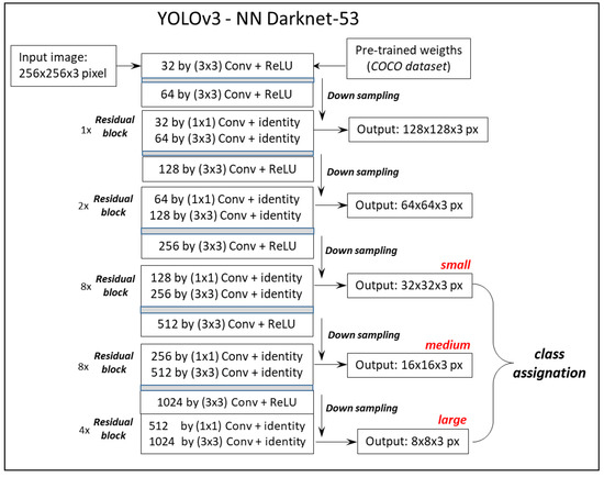
Figure 1.
Schematic representation of the YOLOv3 model implemented with the neural network Darknet-53.
After every convolutional layer, a residual group consists of a series of repeated residual blocks as 1×, 2×, 8×, 8× and 4×. These refer to the number of times each layer of the sequence is repeated, and therefore they can be considered an indicator of the depth of the neural network. In the last three residual groups, the original input image becomes down-sampled at three different resolutions of 32 × 32, 16 × 16, and 8 × 8 pixels (small, medium, and large, respectively) to prevent the loss of low-level features and improve the ability to detect smaller objects (Figure 1). The use of residual blocks is aimed at avoiding saturation when increasing the number of convolutional layers [25]. The last step of the detection process consists of combining low-level features (8 × 8 pixels), detected in the last layers of the network, with high-level features (32 × 32 pixels), detected in the previous layers of the network [26], using a methodology similar to the feature-pyramid network (FPN), where large-scale features and medium-scale features are up-sampled to detect medium-scale objects and small-scale objects, respectively.
Compared to other R-CNNs (recurrent convolutional neural networks), YOLOv3 is definitely faster [16,27]. This is possible because YOLOv3 does not split the object-recognition process into multiple phases but rather produces a bounding box, inside which the probability and class of each object detected in the image are estimated. Despite the high speed in object detection, YOLO suffers from a reduced accuracy in localizing small-dimensional objects.
Three anchor boxes (or bounding boxes) are predicted for each layer, obtained from down-sampled features at three different resolutions of 32 × 32, 16 × 16, and 8 × 8 pixels, respectively. An anchor box is a bounding box of multiple aspect ratios pre-defined using the training dataset (COCO) by running a K-means partitioning algorithm among the possible available choices of identified objects. For each anchor box a prediction is made for (a) the centroid coordinates (x,y), as well as the width and height (w and h, respectively); (b) the objectness score to indicate whether the considered box contains an object (0 if it contains objects, 1 if it does not); and (c), the class probabilities, indicating which class the box belongs to (i.e., faces, cats, dogs, cups, etc.). Since the YOLOv3 model is trained with the COCO dataset, we can have up to 80 possible different classes to which objects can be assigned. However, the number of anchor boxes is reduced with the non-maximum-suppression algorithm (NMS, see below) to highlight the box that best overlays the detected object. The model also evaluates the accuracy of the dimension and localization of the bounding box with respect to the object itself. This is evaluated through the intersection over union (IoU) [28], defined as:
where is the ratio between the extensions of the intersection and the union of the ground truth and the predicted box.
The computer-vision model identifies objects that are highlighted with bounding boxes. These boxes are represented by the coordinates of the object in the image over which the rectangular region is built through the hand choice of the aspect ratio as well as the hand choice of the possible labels of the bounding boxes. This process is carried out by manually tagging about 100 images to be used as the ground truth. A comparison is then carried out between the ground truth and the real person(s) belonging to the tagged test images. A detected person is linked to a particular ground-truth object if there is a minimum ratio of 50% between the overlap and the union of the detected bounding box with the ground-truth bounding box (see Equation (1)). Therefore, the ground truth refers to the bounding box defined around the real object (person). More precisely, ground-truth bounding boxes are a priori defined by specifying center coordinates and dimensions of the rectangular region enclosing the targeted objects. The image dataset is divided into a training set to train the object detector and a testing set to validate it. Both the training and testing sets consist of the actual images and the bounding boxes associated with the objects in the image.
IoU values close to 1 indicate a good correspondence between ground truth and prediction. This can also be considered an index to determine how much the ground-truth box overlaps with the anchor box. The probability that an object is enclosed within the bounding box is called the confidence score and is defined as:
where P(Object) is the a priori probability of finding the object in the box. As said above, for each grid scale the model predicts three anchor-bounding boxes, and therefore multiple anchor boxes could predict the same object. To overcome this issue, the non-maximum-suppression (NMS) algorithm is applied to remove possible duplicate results. Basically, this method determines the detection box characterized by the highest object-confidence score, higher than a given threshold, and adds it to the result while removing all other boxes with a lower IoU. Therefore, the final detection step assigns only one bounding box to each identified person, as shown in Figure 2. In the present work, a confidence-threshold value of 0.7 and an NMS threshold of 0.5 were chosen. The detection range is the result of fine tuning the computer-vision model to detect and track the largest number of targeted pedestrians over consecutive images. We have observed that an increase in detection range is not always followed by correct tracking of the targeted person. Therefore, a compromise was found between detection and tracking accuracy to build the time path of pedestrians. The obtained predicted bounding boxes correspond to the probability that, for the detection of the pedestrian, the obtained object corresponds to the class of “person”. Therefore, the individual bounding-box confidence prediction is defined as:
where indicates the probability of finding a person within the bounding box.
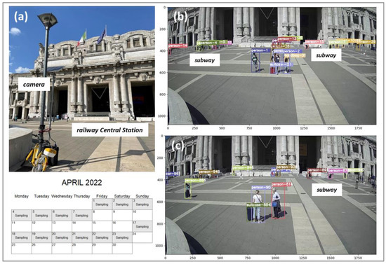
Figure 2.
(a) Camera system for video collection located in the middle of the square Piazza Duca d’Aosta at Centrale Station in Milan, Italy. (b,c) Sample frames extracted from a video sequence. Bounding boxes indicate successfully detected people in the image within a time interval of 10 ms. Each bounding box is associated with a unique identifier.
2.2. Tracking Model
Object detection across frames in a video sequence raises the issue of performing multiple-object tracking (MOT). Tracking algorithms assign unique tracking IDs to every object found in each frame and try to maintain the same ID in subsequent frames using some sort of correspondence.
To track IDs assigned to pedestrians, we applied the SORT model as a tracking framework focusing on frame-to-frame prediction and association [29]. In this model, the inter-frame displacement of each object is approximated with a linear velocity independent of any other object in the video [30]. Tracking of a pedestrian is initialized when the correspondence between the real position of the pedestrian (ground truth) and its prediction is larger than a threshold value . In that case, a tracker is initialized as a bounding box with an initial velocity set to zero. At each time step, a prediction is made for each target’s bounding box considering previous steps. Trackers are usually terminated if the associated target is not detected in the subsequent frame. Figure 2b,c show an example of a detected person whose assigned ID was tracked along their trajectory while walking across Piazza Duca d’Aosta in front of Centrale Station in Milan. Figure 3 shows a typical case in which a detected ID is tracked in several consecutive frames until it disappears. For each ID, a time series is built, including the centroid of the detected person and the timestamp (Figure 4).
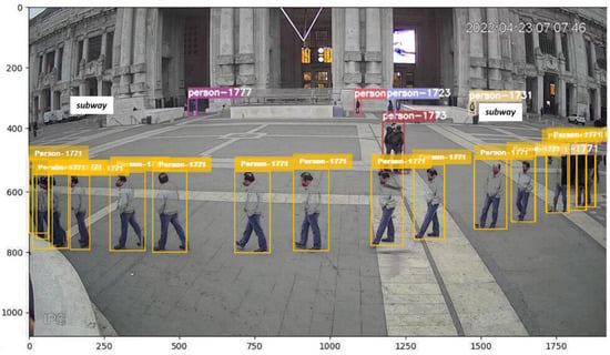
Figure 3.
Example of a sequence of bounding boxes tracking a detected person with their ID maintained along the trajectory. For illustration purposes and clarity of the tracked path, only 2 frames per second are shown. Two entrance points of the subway are indicated. Axis labels refer to the pixel scale of the image.
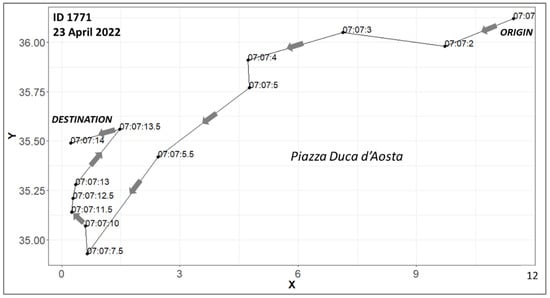
Figure 4.
Example of a tracked ID along its trajectory. For illustration purposes and clarity of the tracked path, only 2 frames per second are shown. Axis labels refer to the metric system, epsg = 32,624.
To characterize the movement of a pedestrian walking across the square, it was necessary to switch from a 3D- to a 2D-view representation (from pixels to meters) and re-project the centroid coordinates to the metric system. This allowed us to observe the path followed by the tracked person at several timestamps. Figure 4 shows the trajectory followed by a tracked ID at a time resolution of 1 second. The sequence of the timestamps defines the position at the beginning of detection (origin) and the position at the end of detection (destination). The direction of each track was defined as the angle between its origin and destination.
3. Experimental Setup
As already stated, the study area chosen for our analysis was Piazza Duca d’Aosta in Milan, Italy, located in front of Milan Centrale Station. The area represents one of the strategic multimodal hubs of the city. With about 600 trains a day, Centrale Station is currently the second largest station in Italy in terms of size and traffic volume. Visited by more than 350,000 people per day, besides offering high-speed railway and lines to other European countries, the station is an interchange spot for buses, trams, trolleybuses, and two subway lines, as well as airport shuttles. The surrounding area hosts taxi and other mobility services such as bikes, scooters, and car sharing. The station has three large central entrance doors facing the main square, Piazza Duca d’Aosta, where two access points to the subway are located.
The dataset used to characterize pedestrian mobility over Piazza Duca d’Aosta consisted of a collection of videos recording the square with a strong perspective view, showing the flow of people around the main entrance of the station and the two access points of the subway (Figure 2a). For this purpose, a video-recording system was setup along one side of Piazza Duca d’Aosta facing the main entrance of Milan Centrale Station. The main purposes of this system were (a) to collect the video streaming coming from a camera adopting standard internet protocol, (b) to process a video stream by analyzing each frame, (c) to detect the presence of people within the frame, (d) to assign a unique identifier (ID) to each person, and (e) to track each person inside every video frame.
The camera was set up by the Azienda Mobilità Ambiente e Territorio (AMAT), with the purpose of acquiring the video stream from Piazza Duca d’Aosta and counting and analyzing the movements of pedestrians. Most of the video streaming was processed offline. The system was programmable remotely and could be controlled through a dedicated app [31]. The video stream was set to capture video in MP4 format in HD through an IP camera connected to a 4G router with a SIM card and a remotely reachable DDNS profile. The video stream had a frequency rate of 20 fps and was analyzed for a period of 14 days during the month of April 2022. The system power was supplied by an 80 W solar panel with a direct current of 12 V that was also charging a 12V, 75 Ah gel battery. The camera was mounted on the end of a telescopic pole that extended up to 4 m. The location of the camera was chosen to cover a wide view of Piazza Duca d’Aosta to detect and track pedestrians entering the station or accessing public transportation. Videos were recorded during 14 days, from 1 to 7 April and from 17 to 23 April 2022 between 07:00 and 20:00. We chose not to analyze any image during days with adverse weather conditions, since the number of people in the observation area was very low. Consequently, it was not possible to provide an estimation of the detection and tracking accuracy in those conditions. With respect to the previous work characterized by a similar methodology [10], this work is based on different dates, and the data collected for the analysis described in the following sections are more homogeneous, since the entire analysis was performed on the same dataset.
4. Metrics
To estimate the mean pedestrian speed, direction, and density over the study area, the capability to detect pedestrians in static images was assessed through the mean-average-precision (mAP) evaluation metric. As said above, a threshold value for the IoU of 0.5 was initially set to establish whether a pedestrian was detected or not, classifying the object as true positive (TP) or false positive (FP) in the case of IoU > 0.5 or < 0.5, respectively. If the ground truth was present in the image but the model failed to detect the object, it was classified as false negative (FN).
The average precision is usually defined as . In general, the mean average precision at IoU = 0.5 (mAP50) is calculated as the mean average precision of all the different classes of objects detected within a single image, based on the following expression:
where N is the number of classes, which is equal to 80 in YOLOv3, and is the average precision for a single class of detected objects. The results, presented in Figure 5, showed a confidence score of about 67.6%. The IoU distribution showed a mean value of about 81%, whereas the mAP50 showed a mean value of about 61%.
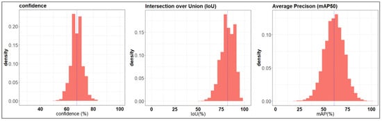
Figure 5.
Distribution values obtained for 3 metrics used to evaluate the YOLOv3 model performance over the observations: confidence of the detection for the class “pedestrian” (), intersection over union (IoU), and mean average precision at IoU = 0.5 (mAP50) for the class “pedestrian.” Results refer to an observation period of 14 days during the month of April 2022. Blue dotted lines represent the mean value of the distributions.
Evaluation of multiple-object tracking was carried out with the standards Multiple Object Accuracy Tracking (MOTA) and Multiple Object Tracking Precision (MOTP) [32]. MOTA [33] is one of the most widely used metrics in object tracking. This metric matches the ground truth (GT) to predicted objects per detection. It considers the number of identity switches, false-positive (FP) detections, and false-negative (FN) detections across all video frames and is defined as:
where MID is the mismatch error occurring when the object in the ground truth is erroneously associated with another object due to wrong tracking. Basically, MOTA measures the overall accuracy of both the tracker and the detection and can be considered a measure of the tracker’s performance at detecting objects and maintaining their trajectories. In general, assuming that MOTA values are usually normally distributed, with a mean value larger than 80%, many of the objects are considered tracked. On the contrary, with a mean value between 20 and 80%, objects are considered partially tracked.
However, MOTA does not consider localization, which must be measured by a separate metric, such as Multiple Object Tracking Precision (MOTP) [33,34], which averages localization scores across all detections within a video and therefore estimates the accuracy of the detection model in localizing the object with respect to the ground truth:
where TM is the total matches made between ground truth and the detection output. Basically, MOTP shows the ability of the tracker to accurately estimate object positions and, at the same time, to be consistent with trajectories. Well-performed tracking systems have a MOTP close to zero.
Figure 6 shows the distribution of MOTA and MOTP values obtained for all the pedestrians tracked during the detection process. A mean MOTA value of about 56% was observed. This indicates that most of the persons present in the videos were partially tracked [32]. On the other hand, the distribution of MOTP values showed a mean value of about 0.6, which, being close to zero, is an indication that the localization capability of the system was good.
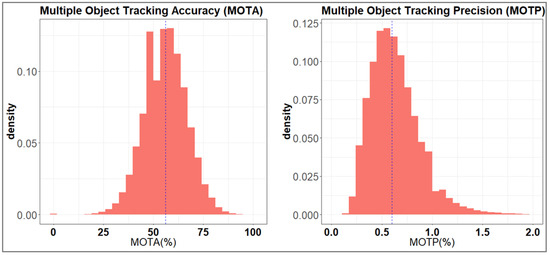
Figure 6.
Distribution values obtained for two metrics used to evaluate tracking precision in the YOLOv3 model: Multiple Object Tracking Accuracy (MOTA) and Multiple Object Tracking Precision (MOTP). Results refer to an observation period of 14 days during the month of April 2022. Blue dotted lines represent the mean value of the distributions.
5. Image Processing
5.1. Speed and Direction
Statistical evaluations were performed after video processing with the computer-vision model, hereafter indicated as CV, to detect and track pedestrians in each frame of the recorded videos. As result, an extensive dataset of about 1.7 million images was gathered during 14 daily timeslots (07:00–22:00) from 1 to 7 April and from 17 to 23 April 2022. Raw data obtained from the CV model consisted of a time series of unique identification numbers (ID) assigned to people targeted in each frame. Raw data referred to a 3D view of the recorded image. Conversion of the coordinates into a 2D view with the ID position expressed in meters was performed using conversion factors dependent on the view angle of the camera, the viewpoint depth of the image, and the top-view dimensions of the observed square, Piazza Duca d’Aosta. The resulting 2D dimension of the observation area had a depth of 45 m and a width of 50 m.
The statistical analysis was structured in two steps: The first one consisted of the visualization of time profiles of the mean number of pedestrians in Piazza Duca d’Aosta during days and hours. The second one consisted of the analysis of the spatial distribution of pedestrian speed, direction, and density over the square by considering two well-defined timeslots: from 07:00 to 10:00 representative of the morning time window, and from 17:00 to 20:00 representative of the evening time window. Indeed, these are the most recurrent time slots of the week when people access the train station and the subway.
The cumulative number of pedestrians was estimated by adding the number of people detected and tracked at each hour of the day (Figure 7). A distinction was made for working days (Monday to Friday) and for the weekend (Saturday and Sunday) during evening and morning hours. The largest number of people was observed during morning hours and during weekdays (Figure 7a). The two-week sampling period highlighted Tuesday as the day with the largest number of people, whereas Sunday showed the lowest number. Analyzing the hourly profiles, a peak in the number of people was observed around 10:00–11:00 both on weekends and on working days (Figure 8b). Another peak was observed around 16:00 but only during working days. On the other hand, a larger number of people was observed around 21:00 during the weekend compared to working days.
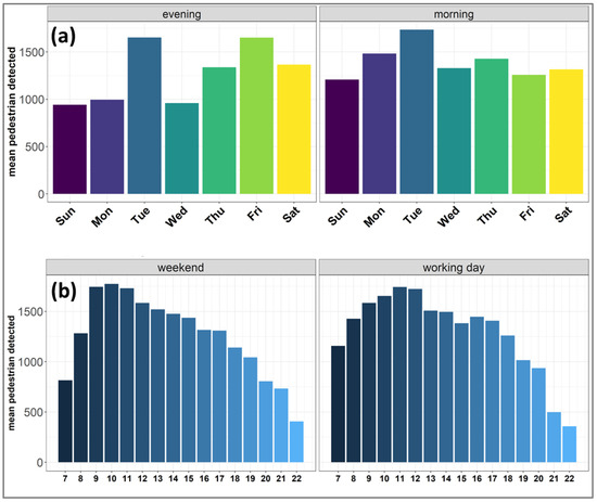
Figure 7.
(a) Daily and (b) hourly profile of the mean (absolute) number of pedestrians in the observed target area.
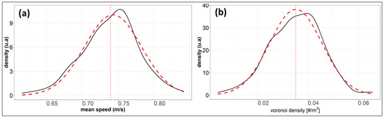
Figure 8.
(a) Distribution of mean speed and (b) Voronoi density during the two-week observation period in April 2022. The ordinate axis label refers to the density distribution, expressed as arbitrary units. Colored dotted lines represent the modeled data distribution.
Pedestrian speed and direction were evaluated from the recurrence of the ID numbers assigned to each person together with the temporal sequence of their position. More precisely, for each ID, speed was estimated considering the distance between two consecutive positions of the pedestrian and the time intercurrent between them. Therefore, the resulting average speed of pedestrian is defined as:
where is the instantaneous speed of pedestrian at the timestamp , is the total of discrete uniform time interval , and, is the space covered by pedestrian at timestamp .
In addition, it was possible to define the temporal distribution of mean speeds related to the overall study area by averaging for the entire pedestrian population the individual speeds at timestamp :
where is the total number of pedestrians at timestamp .
Speeds were filtered to account only for moving individuals () and to exclude bicycles and e-scooters (). Outputs were initially averaged every 15 minutes and then averaged by hour and by day. Daily and hourly profiles of the average speed did not show any significative trend, with the average value ranging from 0.71 to 0.79 m/s and a standard deviation of 0.2 m/s. Overall, speed distribution over the observation period showed a Gaussian shape centered at 0.74 m/s (Figure 8a).
Heat maps were generated to spatially represent pedestrian mean speed and density number. A square grid with a 2 × 2 m2 cell area was overlaid on the observation area to achieve regular tessellation to visualize speed and density values in different parts of the square. This is a different approach with respect to a similar study [10], in which the Voronoi density was computed on the original Voronoi cells, with no reference to the regular grid used in the study.
Instantaneous speeds along each pedestrian trajectory were assigned to every crossed cell. For each cell, daily averages were computed from 30 minute speed averages. In addition, the direction of each trajectory was estimated from the angle, expressed as 0–360°, between the origin and the destination point of each pedestrian. Figure 9 shows that angles were mainly oriented towards two directions: one from the station or subway entrances toward the square (250° < angle < 280°) and one from the square towards the station or subway entrances (80° < angle < 120°) (Figure 9). Therefore, heat maps representing average speed and direction were filtered along these two main directions. The distribution of the angles shown in Figure 9 clearly indicates that the direction followed by the majority of pedestrians was the one from the station or subway entrances toward the square, with higher numerosity observed during the morning hours. However, to better understand and visualize the prevalent direction followed by pedestrians during the morning and evening hours, data clustering was carried out using the well-known K-mean methodology [35] to cluster the whole datasets of speeds and directions estimated during the observation period. The results (Figure 10 and Table 1) show that speed and direction could be grouped into two main categories. The largest numerosity of pedestrians fell within the same clusters during both morning and evening hours. During morning hours, the largest number of pedestrians was directed from the subway towards the square, with an average speed of about 0.77 m/s (Figure 10a), whereas a smaller number of pedestrians was directed towards the entrances to the subway and to the station at a speed of about 0.65 m/s (Figure 10a). On the other hand, during evening hours, the number of pedestrians moving towards the entrances of the subway and the station showed higher numerosity compared to the morning hours, with an average speed of 0.64 m/s (Figure 10b). However, during evening hours most pedestrians were also directed from the entrances to the subway towards the square at a speed of about 0.78 m/s (Figure 10b). It is important to point out that these results may also have been affected by the capability of the YOLOv3 model to better detect and track people along the direction of cluster 1 (see Table 1), therefore potentially resulting in the underestimation of the numerosity along the other directions.
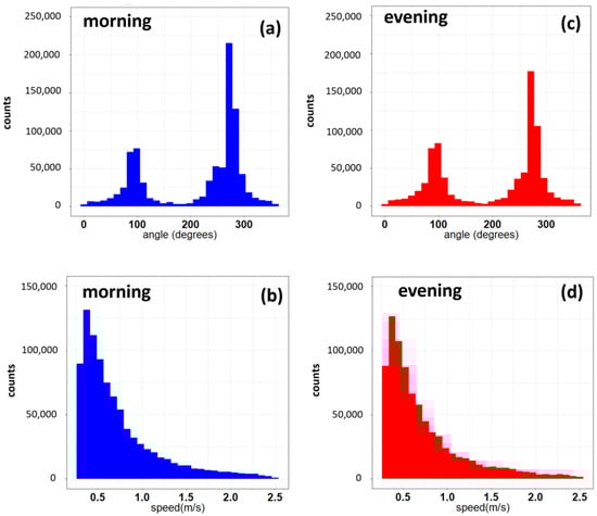
Figure 9.
(a) Distribution of the angles followed by pedestrians during morning (from 07:00 to 10:00) and (c) evening hours (from 17:00 to 20:00) for the entire observation period. The 90° angle corresponds to 12:00. (b,d) Distribution of speeds during the same time windows.
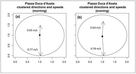
Figure 10.
Clustered speed and directions in (a) the morning (from 07:00 to 10:00) and (b) the evening (from 17:00 to 20:00). The length of the arrows indicates the number of pedestrians for which speed and direction were weighted.

Table 1.
Results obtained from clustering of directions during morning (from 07:00 to 10:00) and evening hours (from 17:00 to 20:00) for the entire observation period. The 90° angle corresponds to 12:00. The numerosity indicates the number of pedestrians classified within each cluster. The average speed for each cluster is also reported in table.
Figure 11a and Figure 12b clearly show that during morning and evening hours, pedestrians mainly used one of the subway entrances in the square when walking towards the station. On the other hand, during evening hours, Figure 11b and Figure 12b clearly show that pedestrians used both subway entrances to leave and walk towards the square. In addition, as shown in Figure 11 and Figure 12, peaks in speed were observed in the proximity of the subway entrances.
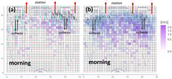
Figure 11.
Heat map of speed across Piazza Duca d’Aosta during the morning (from 07:00 to 10:00) along the (a) entrance and (b) exit direction with respect to the station. Arrows indicate the ending point of a trajectory of a group of pedestrians together with its direction. Results are from two weeks of observations during the month of April 2022. Directions with high standard deviation were omitted. Red arrows indicate the entrances of the station. Grey arrows represent the access points of the subway.
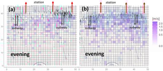
Figure 12.
Heat map of speed across Piazza Duca d’Aosta during the evening (from 17:00 to 20:00) along the (a) entrance and (b) exit direction with respect to the station. Arrows indicate the ending point of a trajectory of a group of pedestrians together with its direction. Directions with high standard deviation were omitted. Red arrows indicate the entrances of the station. Grey arrows represent the access points of the subway.
5.2. Density Analysis
Estimation of pedestrian density was carried out using the Voronoi method. The Voronoi methodology assigns to every pedestrian a cell representing the closest area in order to calculate an arithmetic average of the perceived densities of each user and define the total crowding at a given time [10]. The method requires the Voronoi-cell diagram to be computed for the position of each pedestrian at each timestamp. Since the case study concerned an open area, the boundaries of a square roughly covering the study domain were intersected with the neighboring Voronoi cells to obtain finite areas. Voronoi cells are not of regular size, and they are built around each person by considering the near neighbors. Similar to the estimation of the spatial speed, a grid composed of square grid cells of 2 × 2 m2 was overlaid on the observed area and intersected with the Voronoi cells. In a situation considered homogeneous, densities estimated with the Voronoi methodology do not show considerable variations; on the contrary, they are defined to highlight possible inhomogeneities in the density distribution. This latter condition was apparent during the whole observation period. Therefore, the Voronoi density was estimated considering the ratio between the number of people within each square cell and the total areas of the Voronoi cells intersecting the square cell itself. At timestamp , the Voronoi density for each cell of the regular square grid is defined as:
with
where is the area of the i-th region obtained from the Voronoi tessellation on the basis of the pedestrian position , is the area of each grid cell, and is the normalized weight obtained by sectioning A on the basis of the intersection between the i-th Voronoi cell and the k-th grid cell.
To obtain a global-density indicator of the overall study area, the average space density at timestamp can be estimated as:
where is the total number of grid cells. Finally, to aggregate the density indicators into time-average profiles, the following equation was used:
where is the number of discrete uniform timestamps.
Figure 13 shows the advantage of using the Voronoi-density approach rather than the standard density. The standard density is usually defined as the ratio between the number of people present in a cell and the cell area at a given time. However, the standard density shows higher variability in time with temporal spikes, highlighting the granularity of a single square cell in the temporal variation. Unlike the standard-density definition, the Voronoi method does not show strong oscillations when people enter or exit the measurement area, because in this case every individual produces a density distribution. This yields smoother temporal profiles compared to the standard density, allowing for a better visualization of the temporal variation of the density.
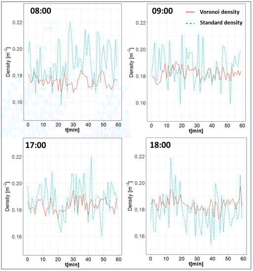
Figure 13.
Time sequence of the Voronoi density and the standard density computed over a square cell in Piazza Duca d’Aosta with high occupancy during the day of 23 April 2022.
For each cell, daily Voronoi-density averages were computed from 15-minute density averages during the whole observation period. Data consistency was assured by averaging the total number of pedestrians crossing each cell within the same time range and by weighting the number of each ID included in the cell with the number of timestamps occurring every minute. This was fundamental to avoiding mismatches when averaging data from different time periods.
Having observed that only a portion of the square was mostly crossed by pedestrians during the observation time, spatial estimation of the Voronoi density was carried out on a square of reduced area. Figure 14 shows that the subway entrances as well the corridors in front of the entrance to the station were characterized by higher densities. This was observed both for morning and evening times. The highest density value observed during morning and evening hours was up to 0.16 person/m2. This result is consistent with the time sequence of the Voronoi density shown in Figure 13. On the other hand, when considering the entire area of the square, the mean value of the Voronoi density was about 0.035 person/m2, with a standard deviation of about 0.014 person/m2 (Figure 8b). This value is consistent with the one found in the previous analysis carried out at the same location during a different time period [10]. Compared to typical results on vehicles, pedestrian densities estimated in this work showed very low variability. In the heat map of Figure 14, the density variability ranged from 0.02 person/m2 to 0.16 person/m2. Therefore, unlike the case of vehicles, the low value for the spread of density was not suitable for performing speed-density plots to estimate the relationship between walking speed and pedestrian density [36]. However, in another recent work [10], we estimated the speed–density relationship for the same pedestrian environment by taking advantage of a microscopic simulator.
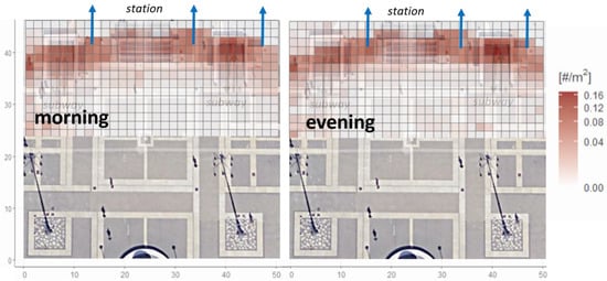
Figure 14.
Heat map of the Voronoi density across Piazza Duca d’Aosta during the morning (from 07:00 to 10:00) and the evening (from 17:00 to 20:00) hours during the whole observation period and over the most crowed part of the square. Blue arrows indicate the entrances of the station.
From the daily profile shown in Figure 15a, low pedestrian density was observed during Saturday evening and Monday morning, whereas high density was observed during Monday evening and Tuesday morning. On an hourly basis, during the weekend, density values started decreasing during the evening from 20:00 to 22:00. On the other hand, during working days, no hourly trend was observed in the density, with only one peak around 14:00, and density values decreased during the evening from 20:00 to 22:00 (Figure 15b).
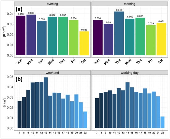
Figure 15.
(a) Daily and (b) hourly profile of the mean Voronoi pedestrian density inside the observation area. Morning time ranges from 07:00 to 10:00, whereas evening time ranges from 17:00 to 20:00.
6. Conclusions
In this work, we illustrated the implementation of an algorithm of computer vision that analyzes images extracted from video frames recorded in front of the Centrale Station in Milan, Italy. The goal was to provide an estimate and a visual representation of speed, direction, and density of pedestrians walking across the square. Tracking and detection of pedestrians was achieved with discrete accuracy. The results clearly show that the main directions followed by pedestrians are linked to points of interest, such as the entrances to the subway and to the railway station. In addition, temporal characterization of pedestrian number and density highlighted the different pedestrian behavior during weekdays compared to weekends.
Even though it was not possible to experience high-flow conditions over the analyzed area, the system can be used offline in the preparedness phase, serving as a support to plan big events. Furthermore, the outcomes of this system can potentially provide useful information for commercial actors such as retailer or entertainment marketing statistics.
The present work highlights some strong points but also has some caveats. One strong point is represented by the value of an autonomous video-recording system: The self-sufficient operating mode does not need any connection to the power grid or any data transfer through a wired network. However, the configuration of the camera plays a key role in obtaining reliable and accurate data. Differences with respect to the results obtained in a previous similar work [10] are related to the different period of observation, when a lower number of pedestrians was detected. Moreover, more work needs to be performed to test the results with different settings of the camera in order to study the possible bias related to uneven spatial distribution of the detection and tracking performance.
Finally, data provided by the camera system and the methodology described in this paper can be useful for both mobility managers and security personnel. Detection and tracking of pedestrians are becoming a popular topic to control mass movements to ameliorate accessibility to public areas as well as to maintain a safe environment. Furthermore, the advancement of new high-performing versions of the YOLO tracking algorithm can significantly enhance the accuracy in estimating the key quantities required to characterize pedestrian-flow dynamics.
Author Contributions
Conceptualization, F.K., C.L., A.D. and M.N.; methodology, F.K., C.L., G.V. and M.N.; software, F.K. and A.D.; validation, F.K., C.L. and M.C.; formal analysis, F.K., C.L., A.D. and M.N.; data curation, F.K. and A.D.; writing—original draft preparation, F.K.; writing—review and editing, F.K., C.L. and M.C. All authors have read and agreed to the published version of the manuscript.
Funding
This research received no external funding.
Institutional Review Board Statement
Not applicable.
Informed Consent Statement
Pedestrian consent was waived due to the fact that images have been treated in order to guarantee at any stage of the data analysis the anonymity of each person involved. To inform pedestrians, a signpost indicating that the images were used in the framework of the research project CityFlows (https://cityflows-project.eu, accessed on 8 June 2023) has been placed below the camera.
Data Availability Statement
Data cannot be publicly shared.
Acknowledgments
The authors would like to thank AMAT—the Environmental Mobility and Territory Agency of Milan, Capgemini, and the project CityFlows for their support in developing and assessing the experimental framework.
Conflicts of Interest
The authors declare no conflict of interest.
References
- Zou, Z.; Shi, Z.; Guo, Y.; Ye, J. Object Detection in 20 Years: A Survey. arXiv 2019, arXiv:1905.05055. [Google Scholar] [CrossRef]
- He, K.; Gkioxari, G.; Dollár, P.; Girshick, R. Mask R-CNN. arXiv 2018, arXiv:1703.06870. [Google Scholar] [CrossRef]
- Wu, Q.; Shen, C.; Wang, P.; Dick, A.; van den Hengel, A. Image Captioning and Visual Question Answering Based on Attributes and External Knowledge. IEEE Trans. Pattern Anal. Mach. Intell. 2018, 40, 1367–1381. [Google Scholar] [CrossRef] [PubMed]
- Kang, K.; Li, H.; Yan, J.; Zeng, X.; Yang, B.; Xiao, T.; Zhang, C.; Wang, Z.; Wang, R.; Wang, X.; et al. T-CNN: Tubelets with Convolutional Neural Networks for Object Detection from Videos. IEEE Trans. Circuits Syst. Video Technol. 2018, 28, 2896–2907. [Google Scholar] [CrossRef]
- Butenuth, M.; Burkert, F.; Schmidt, F.; Hinz, S.; Hartmann, D.; Kneidl, A.; Borrmann, A.; Sirmacek, B. Integrating pedestrian simulation, tracking and event detection for crowd analysis. In Proceedings of the 2011 IEEE International Conference on Computer Vision Workshops (ICCV Workshops), Barcelona, Spain, 6–13 November 2011; pp. 150–157. [Google Scholar]
- Liberto, C.; Nigro, M.; Carrese, S.; Mannini, L.; Valenti, G.; Zarelli, C. Simulation framework for pedestrian dynamics: Modelling and calibration. IET Intell. Transp. Syst. 2020, 14, 1048–1057. [Google Scholar] [CrossRef]
- Sundararaman, R.; De Almeida Braga, C.; Marchand, E.; Pettré, J. Tracking Pedestrian Heads in Dense Crowd. In Proceedings of the 2021 IEEE/CVF Conference on Computer Vision and Pattern Recognition (CVPR), Nashville, TN, USA, 20–25 June 2021; pp. 3864–3874. [Google Scholar]
- LeCun, Y.; Bengio, Y.; Hinton, G. Deep learning. Nature 2015, 521, 436–444. [Google Scholar] [CrossRef]
- Steffen, B.; Seyfried, A. Methods for measuring pedestrian density, flow, speed and direction with minimal scatter. Phys. A Stat. Mech. Its Appl. 2010, 389, 1902–1910. [Google Scholar] [CrossRef]
- Dumitru, A.; Karagulian, F.; Liberto, C.; Nigro, M.; Valenti, G. Pedestrian analysis for crowd monitoring: The Milan case study (Italy). In Proceedings of the MT-ITS 2023 8th International Conference on Models and Technologies for Intelligent Transportation Systems, Nice, France, 14–16 June 2023. [Google Scholar]
- Lu, Y.-J.; Tang, Y.-Y.; Pirard, P.; Hsu, Y.-H.; Cheng, H.-D. Measurement of Pedestrian Flow Data Using Image Analysis Techniques. Transp. Res. Rec. 1990, 1281, 87–96. [Google Scholar]
- Jiao, D.; Fei, T. Pedestrian walking speed monitoring at street scale by an in-flight drone. PeerJ Comput. Sci. 2023, 9, e1226. [Google Scholar] [CrossRef]
- Tokuda, E.K.; Lockerman, Y.; Ferreira, G.B.A.; Sorrelgreen, E.; Boyle, D.; Cesar-Jr., R.M.; Silva, C.T. A new approach for pedestrian density estimation using moving sensors and computer vision. ACM Trans. Spat. Algorithms Syst. 2020, 6, 1–20. [Google Scholar] [CrossRef]
- Ismail, K.; Sayed, T.; Saunier, N. Automated Collection of Pedestrian Data Using Computer Vision Techniques. 2009. Available online: http://n.saunier.free.fr/saunier/stock/ismail09automated-tac.pdf (accessed on 8 June 2023).
- Redmon, J.; Divvala, S.; Girshick, R.; Farhadi, A. You Only Look Once: Unified, Real-Time Object Detection. arXiv 2016, arXiv:1506.02640. [Google Scholar] [CrossRef]
- Redmon, J.; Farhadi, A. YOLOv3: An Incremental Improvement. arXiv 2018, arXiv:1804.02767. [Google Scholar]
- Nepal, U.; Eslamiat, H. Comparing YOLOv3, YOLOv4 and YOLOv5 for Autonomous Landing Spot Detection in Faulty UAVs. Sensors 2022, 22, 464. [Google Scholar] [CrossRef]
- Lin, T.-Y.; Maire, M.; Belongie, S.; Bourdev, L.; Girshick, R.; Hays, J.; Perona, P.; Ramanan, D.; Zitnick, C.L.; Dollár, P. Microsoft COCO: Common Objects in Context. arXiv 2015, arXiv:1405.0312. [Google Scholar] [CrossRef]
- Kerner, B.S.; Rehborn, H.; Aleksic, M.; Haug, A. Recognition and tracking of spatial–temporal congested traffic patterns on freeways. Transp. Res. Part C Emerg. Technol. 2004, 12, 369–400. [Google Scholar] [CrossRef]
- He, K.; Zhang, X.; Ren, S.; Sun, J. Deep Residual Learning for Image Recognition. arXiv 2015, arXiv:1512.03385. [Google Scholar] [CrossRef]
- Jastrzębski, S.; Arpit, D.; Ballas, N.; Verma, V.; Che, T.; Bengio, Y. Residual Connections Encourage Iterative Inference. arXiv 2018, arXiv:1710.04773. [Google Scholar] [CrossRef]
- Szandała, T. Review and comparison of commonly used activation functions for deep neural networks. In Bio-Inspired Neurocomputing; Bhoi, A.K., Mallick, P.K., Liu, C.-M., Balas, V.E., Eds.; Studies in Computational Intelligence; Springer: Singapore, 2021; Volume 903, pp. 203–224. ISBN 9789811554940. [Google Scholar]
- Bochkovskiy, A.; Wang, C.-Y.; Liao, H.-Y.M. YOLOv4: Optimal Speed and Accuracy of Object Detection. arXiv 2020, arXiv:2004.10934. [Google Scholar]
- Wang, C.-Y.; Bochkovskiy, A.; Liao, H.-Y.M. Scaled-YOLOv4: Scaling Cross Stage Partial Network. In Proceedings of the IEEE/CVF Conference on Computer Vision and Pattern Recognition (CVPR), Nashville, TN, USA, 20–25 June 2021; pp. 13029–13038. [Google Scholar]
- Balduzzi, D.; Frean, M.; Leary, L.; Lewis, J.P.; Ma, K.W.-D.; McWilliams, B. The Shattered Gradients Problem: If resnets are the answer, then what is the question? arXiv 2018, arXiv:1702.08591. [Google Scholar] [CrossRef]
- Zeiler, M.D.; Fergus, R. Visualizing and understanding convolutional networks. In Proceedings of the Computer Vision—ECCV 2014; Fleet, D., Pajdla, T., Schiele, B., Tuytelaars, T., Eds.; Springer International Publishing: Cham, Swirzerland, 2014; pp. 818–833. [Google Scholar]
- Lin, T.-Y.; Goyal, P.; Girshick, R.; He, K.; Dollár, P. Focal Loss for Dense Object Detection. arXiv 2018, arXiv:1708.02002. [Google Scholar] [CrossRef]
- Rosebrock, A. Intersection over Union (IoU) for Object Detection. 2016. Available online: https://pyimagesearch.com/2016/11/07/intersection-over-union-iou-for-object-detection/ (accessed on 8 June 2023).
- Bewley, A.; Ge, Z.; Ott, L.; Ramos, F.; Upcroft, B. Simple Online and Realtime Tracking. In Proceedings of the 2016 IEEE International Conference on Image Processing (ICIP), Phoenix, AZ, USA, 25–28 September 2016; pp. 3464–3468. [Google Scholar]
- Kálmán, R. A new approach to linear filtering and prediction problems. J. Basic Eng. 1960, 82, 35–45. [Google Scholar] [CrossRef]
- Dahua Products. Available online: www.dahuasecurity.com/products/All-Products/Network-Cameras/Consumer-Series/2MP/IPC-HFW1235S-W-S2 (accessed on 12 June 2023).
- Bernardin, K.; Stiefelhagen, R. Evaluating Multiple Object Tracking Performance: The CLEAR MOT Metrics. J. Image Video Process. 2008, 2008, 1–10. [Google Scholar] [CrossRef]
- Milan, A.; Leal-Taixe, L.; Reid, I.; Roth, S.; Schindler, K. MOT16: A Benchmark for Multi-Object Tracking. arXiv 2016, arXiv:1603.00831. [Google Scholar] [CrossRef]
- VisAI Labs. Evaluating Multiple Object Tracking Accuracy and Performance Metrics in a Real-Time Setting. Available online: https://visailabs.com/evaluating-multiple-object-tracking-accuracy-and-performance-metrics-in-a-real-time-setting/ (accessed on 22 February 2023).
- Silgu, M.A.; Çelikoğlu, H.B. K-Means Clustering Method to Classify Freeway Traffic Flow Patterns. Pamukkale J. Eng. Sci 2014, 20, 232–239. [Google Scholar] [CrossRef]
- Yang, X.; Zou, Y.; Chen, L. Operation analysis of freeway mixed traffic flow based on catch-up coordination platoon. Accid. Anal. Prev. 2022, 175, 106780. [Google Scholar] [CrossRef] [PubMed]


Disclaimer/Publisher’s Note: The statements, opinions and data contained in all publications are solely those of the individual author(s) and contributor(s) and not of MDPI and/or the editor(s). MDPI and/or the editor(s) disclaim responsibility for any injury to people or property resulting from any ideas, methods, instructions or products referred to in the content. |
© 2023 by the authors. Licensee MDPI, Basel, Switzerland. This article is an open access article distributed under the terms and conditions of the Creative Commons Attribution (CC BY) license (https://creativecommons.org/licenses/by/4.0/).