GIS-Based Model Parameter Enhancement for Urban Water Utility Networks

Abstract

Water utilities are like arteries for the urban environment and, in order to satisfy water demand, extensive design and operation work applying modeling tools is required. An effective tool can be operated but only if the input, such as real-world consumption data, is built into the system. This study aims to present a GIS-based technique to align the consumption data to a simplified network topology. This study investigates four distinct methods, revealing noteworthy outcomes. The geocoding of consumption locations facilitates their seamless integration with model nodes through geospatial methods. Additionally, effective water consumption allocation is achieved by delineating influence ranges around each node. When comparing the zoning based on the street approach and the arithmetic average with the benchmark manual range of influence approach, substantial errors appear of approximately 190% and 230%, respectively. Addressing the impracticality of the manual method, especially for larger networks, this study advocates for the use of Thiessen polygons to delineate influence areas. In conclusion, this study presents a holistic approach to aligning consumption data with simplified network topologies for enhanced water utility modeling.

1. Introduction

Urban water management is a key issue, especially in the planning and operation of water utilities. The efficiency and sustainability of these networks is key to meeting the growing water demand in urban areas. A sustainable approach includes reusing water, promoting resource conservation and environmental responsibility. The emphasis on sustainable practices highlights the need for innovative solutions in urban water management to ensure a resilient and environmentally sound future [1,2].

Due to inadequate or absent maintenance, the technical condition of water utility networks consistently deteriorates [3]. Public water supply is classified among critical infrastructure systems [4], whose resilience must be further developed against natural hazards [5,6], human interventions, and aging [7]. Attention must be given to prioritizing the consistent delivery of services at a high standard. Utility providers are responsible for ensuring an uninterrupted water supply that meets the contracted consumers’ needs in terms of quality, quantity, and pressure. Additionally, used water must be collected and transferred to a treatment system before being discharged into the receiving body of water [8].

The effective utilization of resources necessitates a proactive rather than a reactive strategy with the focus on sustainability [9,10]. There are several studies on the evaluation criteria of sustainability in urban water management, which are applicable to various contexts; a portion of the assessment criteria can be employed for any particular situation and the selection of water supply and demand management alternatives [11] or by introducing a sanitation sustainability index covering technical, social, and economic aspects [12]. Existing sustainability indices, while valuable, may not fully capture the complexities of sustainable urban water management. However, they serve as crucial aggregate parameters, particularly for critical infrastructures and circumstances. To improve effectiveness, integration of emerging factors like climate change and enhancing adaptability to local specifics are vital considerations for refining these indices to better address multidimensional challenges.

The widespread adoption of smart techniques is becoming evident in the water sector, where there is a need to tackle the challenges related to ’big data’ and extracting meaningful insights from the noise. The primary emphasis is on translating data into actionable outcomes through the application of data science [13]. Infrastructure asset management for urban water pipes relies on asset data. Traditionally, most water utilities have not collected the necessary data, leading to low availability, integrity, and consistency. A process is needed to help utilities evaluate and enhance their data management for accuracy and completeness in line with their objectives [14]. To this end, Okwori et al. (2024) created a framework to implement digitalization and embrace data-driven strategies offering practical applications in managing pipe networks [15].

Gilbert et al. (2021) proposed integrating geospatial and geometric data from Building Information Modeling (BIM) and water distribution network models. This integration optimizes dynamic network partitioning, minimizes the risk of underground utility strikes, and plans for future network configurations with higher topological redundancy. The authors introduced a weight-based spatial algorithm demonstrating the application of spatial data for inferring water network connections between urban-scale distribution networks and BIM models, even in the absence of complete or consistent semantic representations [16]. Marzouk and Othman (2020) employed a comprehensive strategy, integrating water consumption, sewage production, and energy consumption within a unified framework. This approach assists city planners and managers in making informed decisions during the initial phases of city development or expansion [17]. Moreover, as an instance of coupling BIM and GIS (Geographic Information System), Sharafat et al. (2021) introduced an integrated framework that enhances underground utility management throughout project life cycles. It comprises a data source layer, a data-processing layer, an integrated BIM-GIS platform, and an application layer, and utilizes advanced surveying techniques for comprehensive surface and underground infrastructure information collection [18]. However, the integrated technology may face technical and organizational challenges. These challenges include reconciling incomplete or obsolete information on underground infrastructure, addressing gaps in digital competences among stakeholders, ensuring seamless interoperability between BIM and GIS systems, and overcoming resistance to change within existing organizational structures. Despite these challenges, the practical impact of such integration can lead to improved decision-making, enhanced infrastructure planning, and ultimately, more sustainable urban development outcomes.

The multifaceted role of GIS in water utility systems is evident in spatial planning and network design [19], asset management [20], and the formulation of emergency responses [21]. The latter aspect holds significant importance in the context of the recent COVID-19 pandemic. This involved monitoring shifts in demand volumes and patterns, potentially prompting adjustments in water infrastructure operations and water quality measures [22]. Several articles emphasize the importance of computational modeling, data-driven analyses, and proficient utilization of Geographic Information Systems (GISs) to enable accurate assessments, predictive simulations, and the recognition of emerging patterns and trends [23]. The main focus lies in converting data into actionable results through the utilization of data science techniques [24].

A well-developed GIS database enhances water quality by optimizing operating parameters, reducing water age, and increasing average flow rates in the water supply network. In the sewerage network, it minimizes infiltration and accidental water while also mitigating the risk of odor nuisance [25] as well as potentially toxic elements in marine-coastal environments [26,27]. A well-constructed data model is crucial for maintaining the stability of a water utility network model based on a GIS. To ensure integrity and robustness, certain restrictions need to be imposed, which can be categorized into two types: topological and non-topological constraints. Topological constraints encompass connections and other geometric limitations, while non-topological constraints exist at different levels, including system-wide, per network, and per entity (e.g., pumps) [28].

The necessity for iterative solution methods in hydraulic modeling arises from the non-linear nature of water flows, which demands a substantial computational effort. To mitigate this effort, Graph Theory is frequently employed to simplify and analyze networks, network forcing, and/or the flow within networks [29]. Calculating typical values for topological metrics allows for the creation of synthetic water distribution network graphs that mirror the topological characteristics of actual water networks and parallel reductions in the size of the network [30].

Although utilizing graph-based networks may decrease computation time, they often oversimplify the transient flow dynamics and responses of pumps and valves. Nevertheless, Kaltenbacher et al. (2002) have presented a promising algorithm that holds the potential for universal applicability across various flow regimes. It is noteworthy, however, that this algorithm has been exclusively applied to a crucial hydraulic parameter, namely, pipe roughness [31]. Furthermore, water utilities are keen to identify a pragmatic solution that can be implemented on a daily basis, offering simplicity and requiring minimal additional data beyond their existing records.

There are relatively few options for providing spatial consumption data when modeling a water utility network [32]. In most cases, the volume supplied to a given area is known, even at a relatively small—hourly—resolution. However, the distribution of this quantity within the area is not easy to approximate. Given the infrastructure in place, the use of metered values would be appropriate. Several municipalities already use remote water meters, which in the future will make it easier to approximate the spatial distribution of consumption [33].

The supplier does not treat consumers differently in terms of their consumption; for some customers, monthly meter reading and billing of the average consumption is used, whereas in other cases, annual meter reading by a water utility employee is involved. The billing systems therefore associate annual consumption values with each consumer, not for a given year, but for a period of almost a year since the last meter reading. These values can therefore only be used as a benchmark. Furthermore, the technical management systems of the service providers are not usually linked to the billing systems; therefore, the consumers’ data are not linked to spatial data but only to address data. The methodology we have outlined, based on geocoding, could provide a solution to this engineering gap. This integration is crucial for optimizing spatial data utilization and improving the accuracy of hydraulic modeling in the context of service provider networks.

In Section 2, the focus is on elucidating the site characteristics concerning water consumption and providing intricate network details. Additionally, this section delves into the methodology employed for geocoding, offering a comprehensive overview of the processes involved. Section 3 presents the outcomes derived from multiple scenarios of topology model simplifications. By simplifying topological models, researchers can focus on local specialties and pertinent aspects of the network, tailoring simulations to address specific objectives. Moreover, the fidelity of the model is contingent upon the quality of incoming data; if data quality is subpar, fine-tuning the model may not significantly improve accuracy. This section not only showcases the diverse results obtained through these simplifications but also conducts a meticulous comparison with existing results. The objective is to discern any variations or improvements brought about by the applied simplification techniques, contributing to a deeper understanding of the network’s behavior and efficiency.

2. Materials and Methods

2.1. Site Desciption

To examine the efficacy of the proposed methodology, a case study was conducted in which a Central European municipality was employed as the testing site. It was selected based on several criteria aimed at ensuring the representativeness and generalizability of the findings. Firstly, the municipality exhibits a typical urban structure commonly found in the Central European region, making it a suitable candidate for studying water distribution network characteristics and behaviors in this geographical context. Additionally, the municipality can be regarded as a segment of a larger urban area, allowing for scalability and the potential to extrapolate findings to similar urban segments. The data were provided by the local utility service and the national Hungarian Central Statistical Office. The administrative expanse of the settlement encompasses 40.74 km², with an internalized zone comprising 40.03 km². The territorial extent of the administrative area has exhibited constancy over the antecedent decadal interval.

The permanent population is 1741 according to the latest data (2022). The population change over the last 20 years is illustrated in Figure 1. Based on the available data, the population of the municipality has increased by 83 persons in the 22-year period under review, which is less than 5% of the total population. The population has been stagnating for the last 10 years. The population density was 44 persons/km².

Figure 2 shows the age and sex distribution of the permanent residents. The data show a relatively stagnant population composition in terms of age groups, which does not allow us to project any change in the long-term water utility forecast.

The housing stock of the municipality also shows a stagnant change over the period under study. Based on Figure 3, one-room dwellings accounted for 18%, two-room dwellings (including one room and a box room) for 46%, three-room dwellings (including two rooms and a box room) for 26%, and even dwellings with four or more rooms (including three rooms and a box room) for 10% of the total housing stock. The area is characterized by single-story detached housing.

In terms of public utilities, telecommunications, electricity, gas, and water are available in the settlement, while sewerage will be provided at a later stage. The majority of the water supply network relevant to this topic is from asbestos cement pipelines built about 40 years ago, which represent approximately 80% of the water main of the distribution network. In addition, utilizing biological processes for asbestos cement waste treatment addresses the pertinent issue of aging infrastructure, particularly in pipes made of this material. This underscores the importance of monitoring maintenance and replacement strategies in effectively managing such infrastructural challenges [34]. The pipelines built in the last 20 years are now polyethylene pipes, which currently represent approximately 20% of the network. The connections to the properties are predominantly steel pipelines and in the first phase of construction; therefore, they have a lifetime of several decades. There are currently five public hydrants in operation in the municipality. The amount and distribution of the water supplied are shown in Figure 4.

According to the most recent data, 91% is billed for domestic use and 9% for other (mainly public) use. The total annual volume is 38,260 m³. Looking at the data for the last ten years, there has been an approximately 24% increase in consumption in the municipality. Furthermore, 397 dwellings are connected to the utility network, resulting altogether in 428 service points.

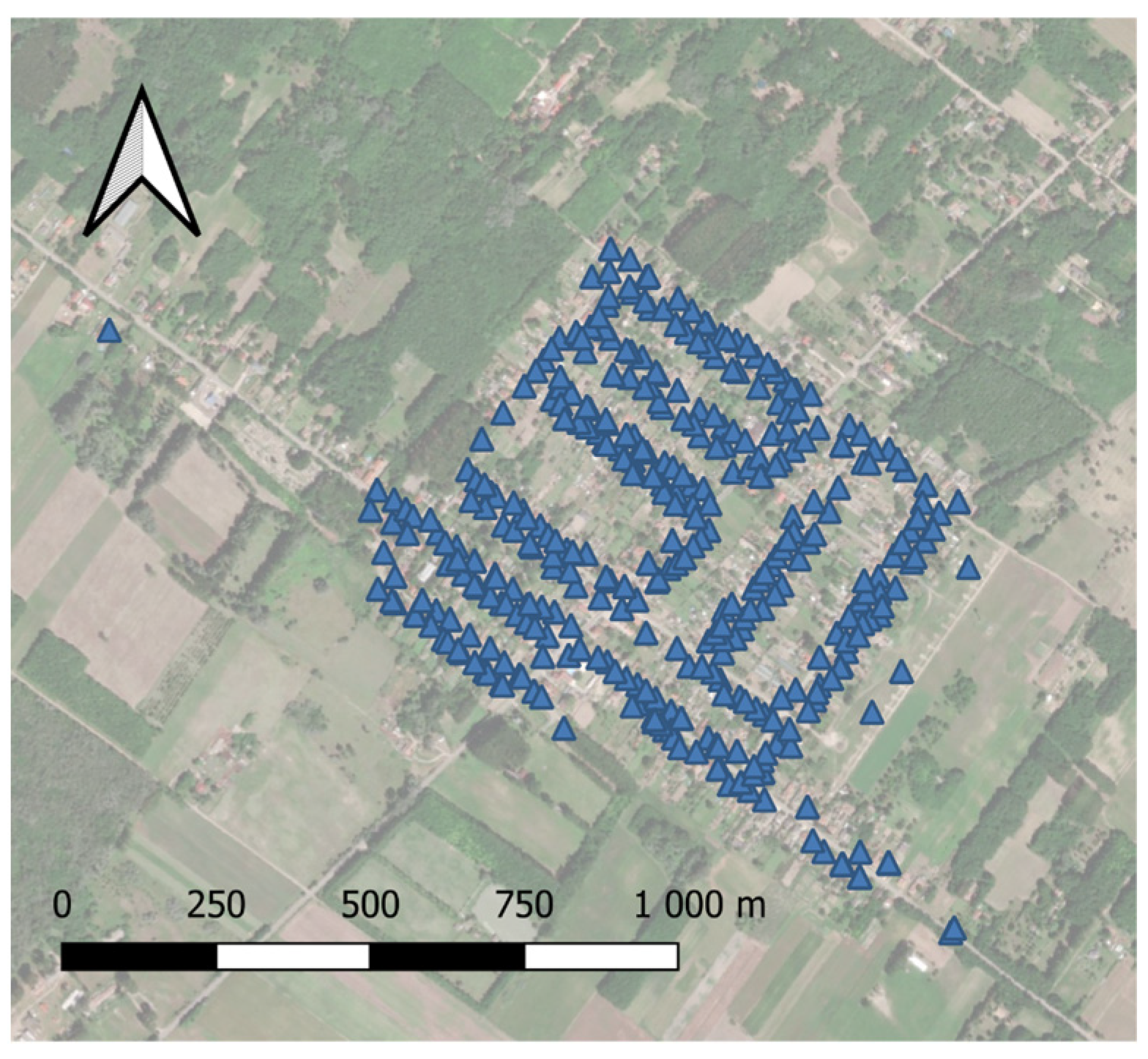
2.2. Geocoding Methodology

For geocoding, the database must be prepared for assigning spatial data to the data obtained from the billing system. The geocoding was performed using the Google address database, which has a defined structure for specifying search parameters [35]. When exporting data from the billing system, the correction of characters due to character encoding discrepancies was performed as a first step. To ensure data integrity and accuracy when correcting characters caused by encoding discrepancies, we employed manual correction methods while adhering to Google’s standards for geocoding. Additionally, given the variability in address standardization and privacy policies, we prioritized transparency and compliance with regulations, especially considering that street and house number information is publicly available.

Data reconciliation includes sanity check (e.g., elimination of public hydrants with negligible consumption), and corrections had to be made for several addresses where no house number was given, only a parcel number. There were three consumption locations in the database that were not found by the Google system, because they were connections to a property built in a completely new street. These locations were included in the subsequent processing. Due to previous search experience [36], where we performed similar searches on nearly 60,000 item numbers with a hit accuracy of over 90%, only 4 incorrect hits had to be manually corrected after the first database search was performed. Including the 3 sites mentioned above, a total of 7 addresses had to be manually entered. Following the correction of these locations, the database geocoding was completed with 100% accuracy. The map representation of the result is shown in Figure 5, where the blue triangles represent the geocoded consumption points.

The great advantage of this method is that it can be carried out relatively quickly. The described processing took 1.5 h. The application on larger databases does not significantly increase the processing time either, because the modification of the specific structure of each database to the desired format can be carried out step by step for the whole database. Only the individual errors (7 address data items) presented in this processing can increase the processing time. It is important to note that the Google address database is constantly updated and offers, therefore, relatively up-to-date data. To minimize the increase in processing time when adapting larger databases to the desired format, we implemented efficient data-structuring techniques and optimized algorithms. Specific errors in address data were addressed through meticulous error handling mechanisms, such as automated error detection and manual verification processes. Leveraging the reliability of Google’s constantly updated address database, we ensured the seamless integration of updated data by regularly syncing our database with the latest information. Furthermore, we embraced the evolving nature of data availability, enabling citizens to contribute to data accuracy through correction requests, ultimately leading to higher accuracies over time.

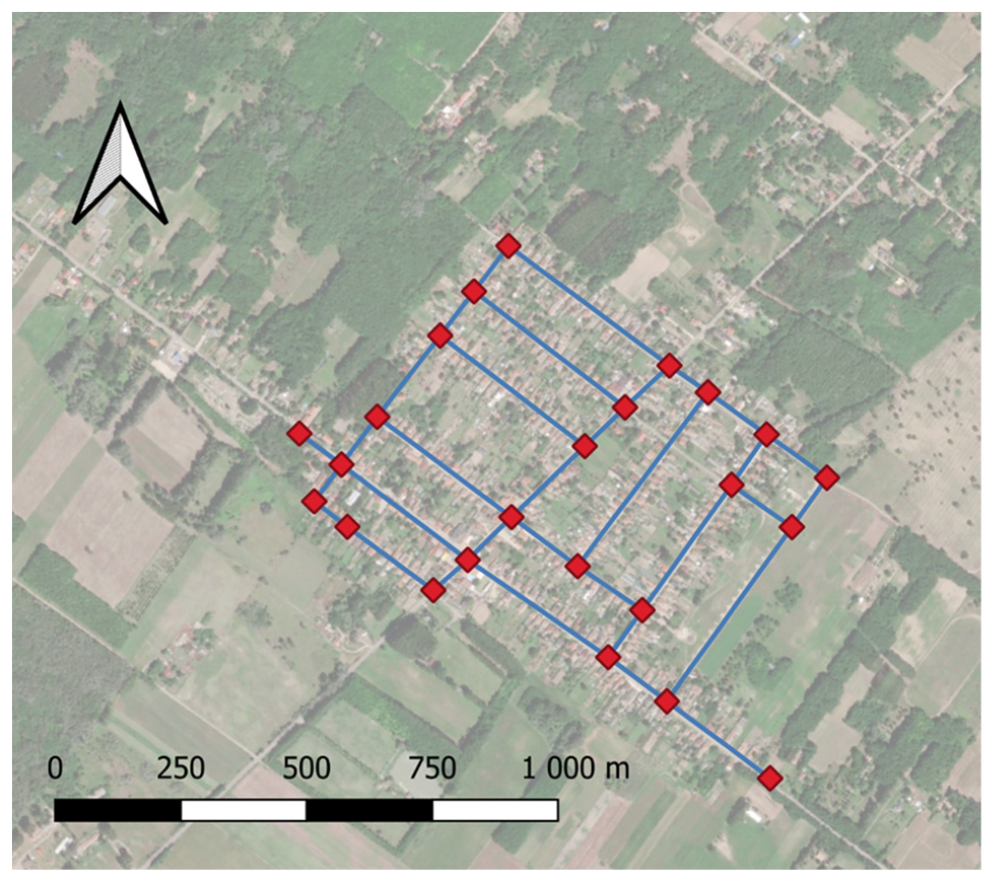
2.3. Topology Simplification Methods for Looped Pipelines

After the geocoding, the spatial distribution of water consumption was carried out to prepare the parameters of the hydraulic model. In practice, a number of methods based on topological simplifications were applied. These simplifications were necessary to run the hydraulic model in a cost-effective way, without requiring large computational resources. These methods may include the arithmetic mean method, division into consumption zones, and consideration of the actual point of consumption [37].

The arithmetic mean method is the simplest quantity distribution method, but it is rarely used in practice. It can be used with a relatively good approximation in places where the street structure of the settlement is uniform, and where there are no major differences in built-up areas and consumption patterns. Gaafar et al. (2019) developed a hazard assessment framework and decision support system to improve the management of point-source pollutants in stormwater effluents and their impact on surface water quality. The framework comprises stormwater hydrological and hydrodynamic simulations, a stormwater quality model for predicting pollutant mass loads and concentrations, a GIS-based model for generating concentration maps [38].

Consumption zones can be defined on the basis of the characteristics of the area. There are practical methods to achieve this, such as zoning by comfort level, zoning by built-up area, zoning by street, and zoning by type of consumer. The idea is to categorize consumers by area and to give the same weight to areas in the same category when allocating consumption.

The separation of areas by comfort level is irrelevant in most municipalities currently, because almost all properties in the study area have a public drinking water service, which, when connected to the residential property, satisfies everyday water needs such as for drinking, cooking, washing, laundry, and toilet flushing. There are several types of zoning by built-up area that can be applied according to the characteristics of the area. The most common are single-family zones, high-rise areas (multi-family housing), and large industrial or public utility areas. In this study, it was applied on the basis of the concentration of water consumption in a given area as a study on the district metered area (DMA) approach suggested [39].

A more accurate result than the methods presented here could be obtained by defining a range for each model node. A relatively quick result could be obtained by summing the lengths of the pipelines connected to the nodes, then taking half of this value and multiplying the resultant value by the length of the whole network of pipes and assigning a weight to each node. The approach could be further developed by applying Thiessen polygons [40,41,42]. The major drawback of this approach is that it only considers the topology of the network and not the actual spatial location of the consumers and the quantities they consume. Its accuracy comes from the assumption that a longer water main length implies more connections and therefore higher consumption.

Without the geocoding described above, recording consumption points at the actual location of consumption would be an extremely time-consuming process. In order to compare the different methods, a base network was created, which allowed us to compare the various approaches. The network aims for a topological minimum, and this is illustrated in Figure 6.

The red squares are the demand nodes of the network and the blue lines are the pipelines of the network. The nodes need to be assigned to consumption data.

3. Results and Discussion

3.1. Arithmetic Mean Method

Applying the arithmetic mean method, the same consumption was allocated to each node, but since the demand nodes are not evenly distributed, the consumption shows an uneven spatial pattern. There were 24 nodes in total, meaning that each node receives 1/24 = 0.0417 of the incoming flow. Figure 7 shows the consumption weights in a heat map.

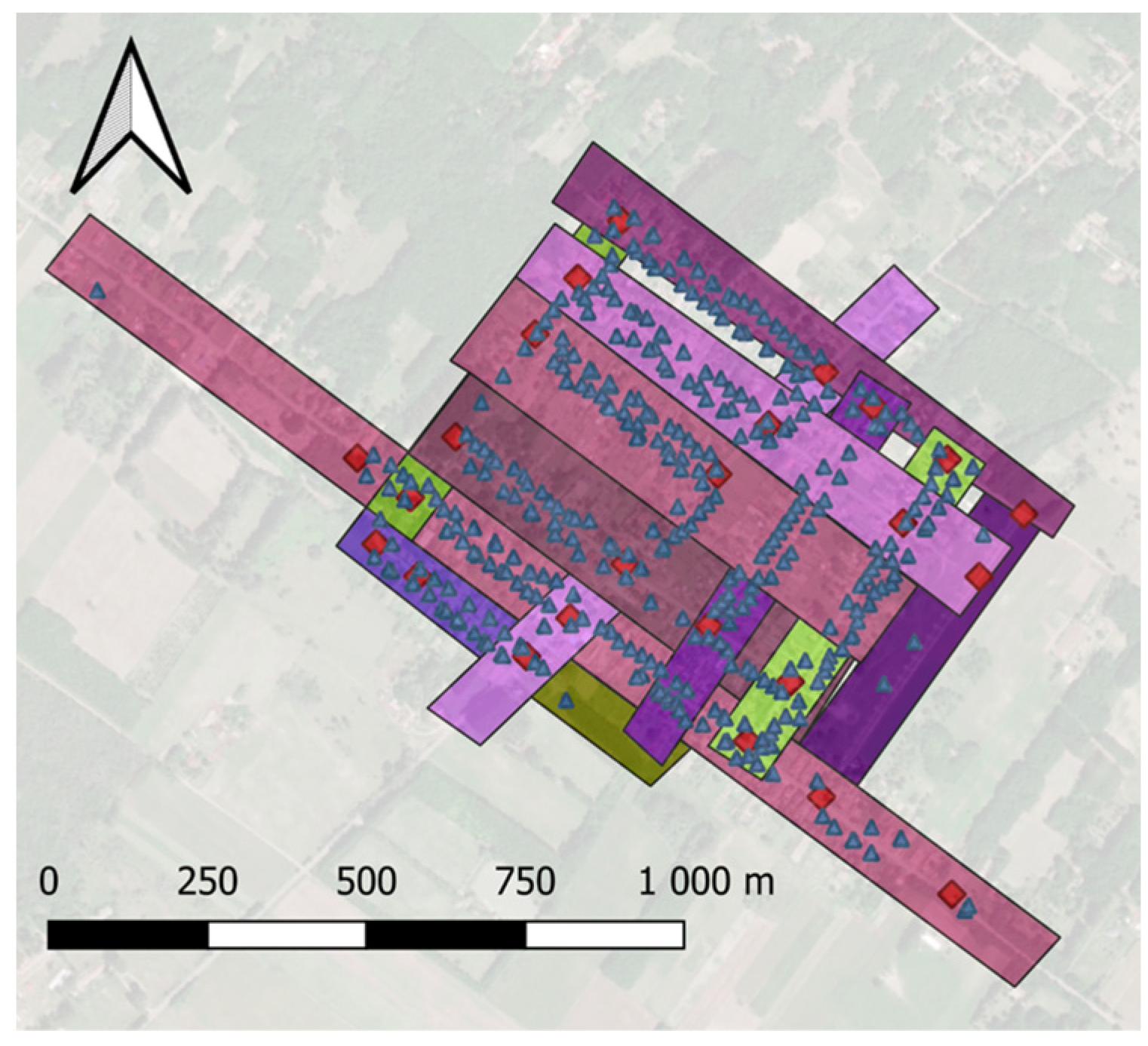
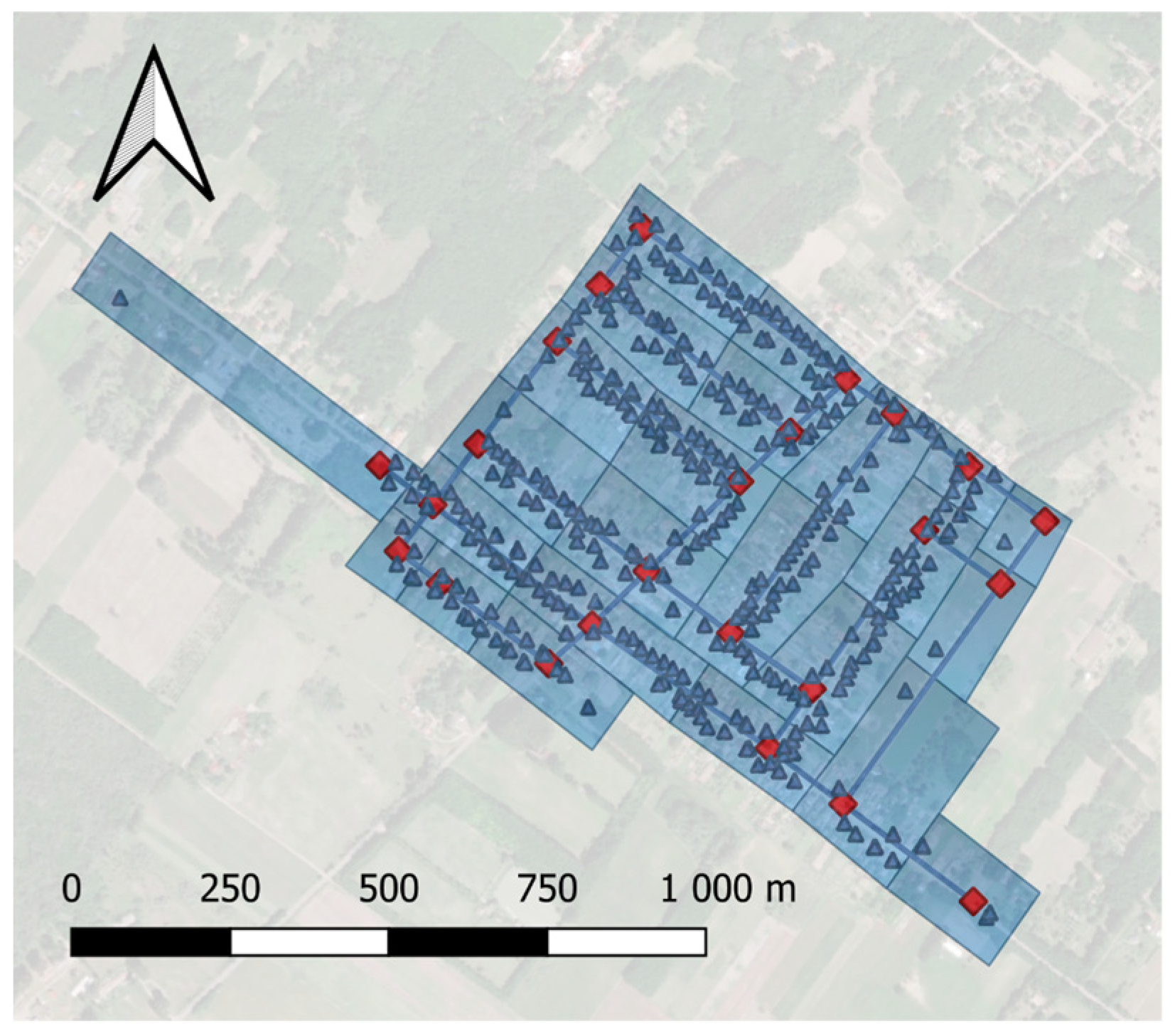
3.2. Zone Delineation Based on Streets

There are no industrial areas, shopping centers, or other local large consumers in the study area. The built-up area shows a relatively uniform pattern. The water distribution network follows the street layout in most cases, the main reason being that the water mains are located in public spaces; therefore, this method is good and relatively quick to implement. Figure 8 shows the division into districts by street. The areas where the network nodes marked by the red rectangles touch several streets at the same time are clearly visible. The processing, therefore, involves summing up the billed volumes for each street and distributing them proportionally to the model nodes in the street. Nodes that affect more than one street will be taken into account for all streets concerned.

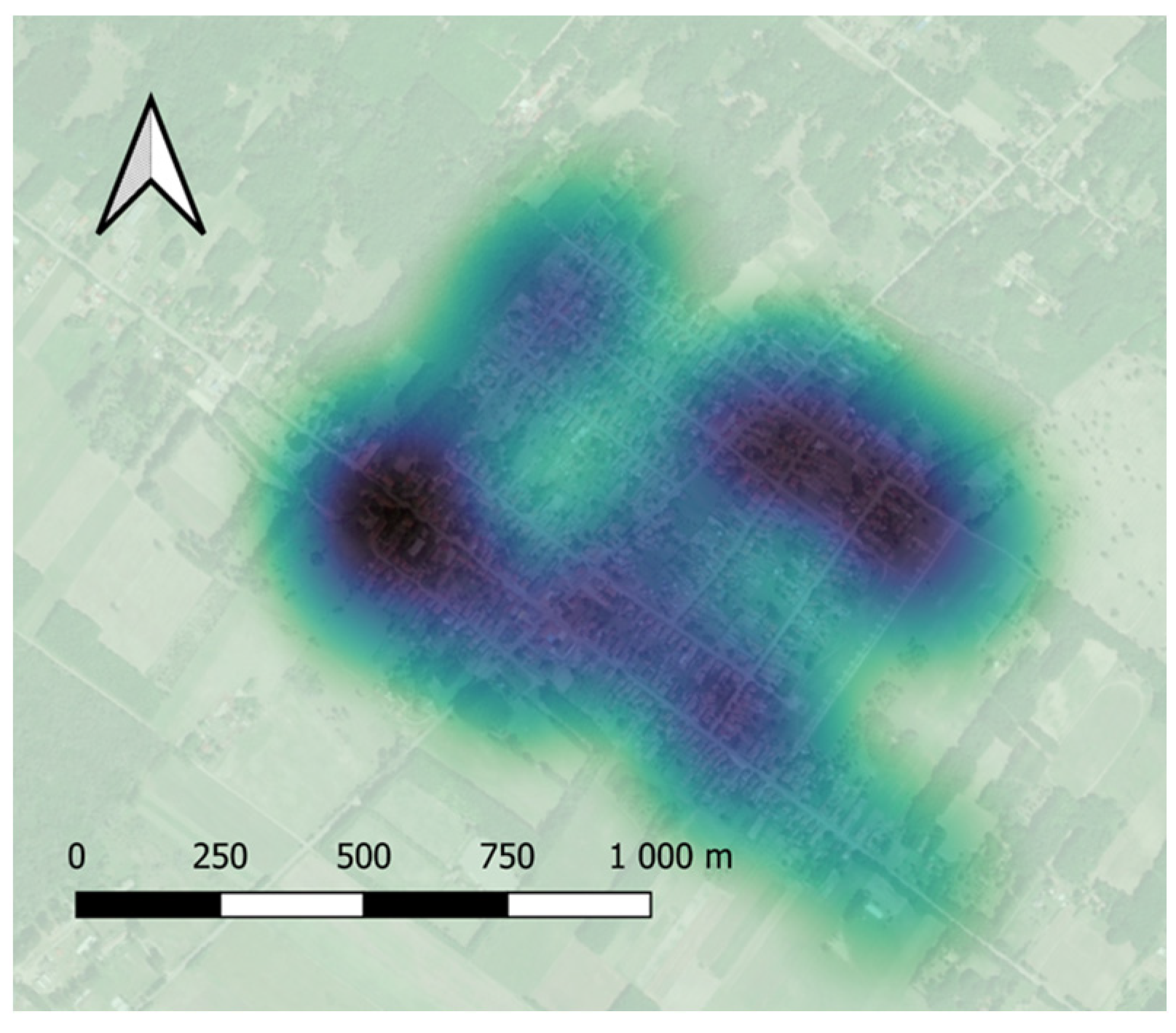
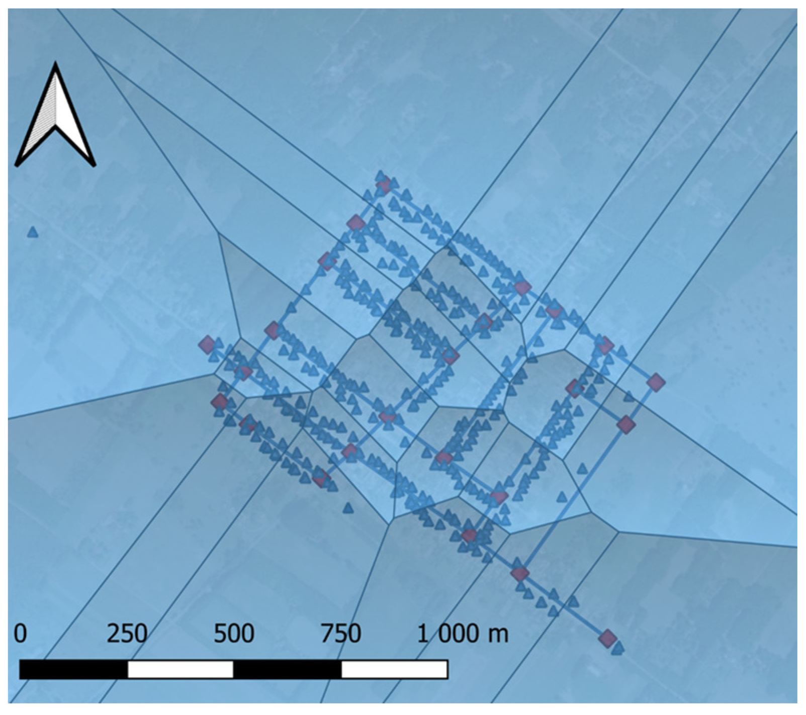
3.3. Consumption Based on the Nodes’ Range of Influence—Manual Method

A more accurate method than proportional consumption is to take into account the actual locations of consumers and use them as the basis for determining the range of influence for each network model node. Figure 9 shows this delineation. It has been constructed to include half the distance between two model nodes and to include all the nodes detected during geocoding. Once the boundary areas have been established, the geocoded consumption locations associated with each node can be easily assigned to the model nodes using a geospatial method. This method allows us to better approximate the number of consumption nodes to reality, and when examining consumption at actual locations, these error possibilities do not arise.

Applying the manual method in this form is extremely time-consuming for larger networks. In our work, we have therefore used the method of delimiting the area of influence with Thiessen polygons. The boundary definition is shown in Figure 10. The method is very similar to the manual method of determining the tangent area due to the structural nature of the polygons. As an example from the literature, Mosbach et al. (2022) applied georeferenced polygons, allowing for flexible transferability to other study areas, to generate practical and sustainable network expansion proposals based on actual topology. This model aligns with our current methodology in this study [43].

Figure 11 shows a map representation of the resulting consumption weights in a heat map. The etalon was the proposed manual method (part A) and the average consumption weight difference ($\overline{∆}$) was calculated as follows: the difference between the nodal value of the selected scenario and the nodal value of the reference (manual method) yields a numerical value. This difference is calculated for each node, and then, an average of these differences is computed.

Zoning based on the street and the arithmetic average method yield similar differences when the average difference is calculated, even though the distribution of weights may not be alike. It is unsurprising that the arithmetic mean consumption weights are evenly distributed among the nodes. However, due to the uneven distribution of nodes, there are slight differences apparent. Conversely, in the scenario involving zoning based on the street, the differences between nodal values and consumption values diverge altogether.

The scenario based on Thiessen polygons’ range of influence closely resembles the manual method. To reveal any differences, each nodal value is compared and depicted in Figure 12.

In some cases (node IDs 0, 3, 5, 18, 20, 21, and 22), there is no difference between the values. The similarity is only due to the locations of the nodes, since each node falls entirely within the area defined by the manual delimitation and the Thiessen polygon delimitation. In comparing Thiessen polygons to the manual method for determining areas of influence, it must be acknowledged that the manual method involves a subjective component and is not fully automated. However, despite this subjectivity, similarities with Thiessen polygon results can be observed. One advantage of the manual method is its flexibility in considering additional factors such as controllers and valves when determining the area of influence.

Evidently, since actual consumption data that reflect reality are employed in the manual method, it is considered to be the most accurate. The automation of the method’s implementation necessitates the utilization of Thiessen polygons, which can be executed rapidly and reliably but may introduce a slight discrepancy.

Comparing the zoning based on the street approach and the arithmetic average to the benchmark manual range of influence approach, we encounter errors of approximately 190% and 230%, respectively. The reason for this is that these methods only consider consumption at the street level or, in some cases, do not account for the real consumption at all. For node ID 23, one property falls within the influence area, but the last billed consumption quantity for that property in the previous year is 0 cubic meters. This is because the house is currently under construction. Both the street-level simplification and the arithmetic average methods failed to account for this situation. To eliminate such errors, the following measures are proposed: on-site visits and critical inspections to validate data accuracy, as well as collaborative efforts between water service providers and billing databases to filter out anomalies effectively. Additionally, ensuring accurate data representation necessitates continuous monitoring and adjustment of zoning strategies to reflect evolving property dynamics.

Figure 13 is a filled contour line plotted using the ratios of the consumption values assigned to the geocoded database values to the whole. It allows the differences in consumption between areas that can be easily examined visually. The lighter parts show areas with lower consumption and the darker parts show areas with higher consumption values.

It can be observed that various methods may result in significant differences in the distribution of water quantities, a point contradicted by Bao and Mays [37]. The discrepancy in system reliability between the arithmetic mean of nodal reliabilities and the weighted mean of nodal reliabilities appears to be insignificant in cases when chessboardlike universal distribution is assumed. Discrepancy arises from relying on an overly idealized and unrepresentative scenario, which does not fully capture the complexities of distribution networks in reality. The extent of the difference greatly depends on the specific urban and consumption structure, being more substantial when encountering asymmetry in both the geometric layout of the urban area and variations in consumption patterns, and this could be even more adverse in the case of high consumers existing in the network.

DMAs partition water networks into smaller sections, with monitoring of the flow in and out of each area. However, a significant limitation of the DMA approach is the diminished redundancy in network connectivity, leading to adverse effects on network resilience, incident management, and deterioration in water quality. Wright et al. (2014) proposed an approach in which the topology is dynamically reconfigured. The method demonstrated in this study can then generate consumption data based on reality for the desired cluster in the new topology [44]. However, the approach applied in this study involves creating flow ratios and determining consumption states (such as daily average, peak, and extremities), followed by distributing the total flow along predefined ratios. This method ensures the generation of consumption data that align with the characteristics of the desired clusters within the new topology, facilitating more accurate simulations and analysis.

As the topological clustering is based on real water demand data, the results could be applied to improve hydraulic modeling of the network aimed at locating sensor placements or isolation of a contaminant intrusion, as Perelman and Osfeld (2011) demonstrated in their study [45].

Geocoding errors were explored in the study by Singh (2017), focusing on discrepancies observed when utilizing Google Sheets and ggmap, two freely available geocoding tools. The research findings highlight the importance of ensuring that addresses are devoid of the ampersand character for accurate geocoding results, with subsequent validation and visualization through various mapping tools recommended to ensure reliable geospatial analysis [46]. Furthermore Chow et al. (2015) stated that disparities in geocoding errors between urban and rural regions varied notably across most geocoding solutions, yet no consistent or monotonic pattern emerged, and excluding the outliers changed the direction of urban versus rural accuracy in most of the geocoding techniques [47].

The applicability of the presented method could be further expanded to sewage collection systems. The water consumption data could be translated to produced wastewater via the sewage generation rate [48]. Duque et al. developed a simplified sanitary sewer topology at urban scale by developing a spatial algorithm, with real-time estimates of wastewater production.

4. Conclusions

In summary, this study explored the intricacies of water utility network simplifications, acknowledging the potential influence of topological constraints on hydraulic and transport modeling. Emphasizing the dependence on real-world data, GIS tools were utilized to connect real-time water consumptions to each demand node. The investigation encompassed four methods, yielding the following results:

• The geocoded consumption locations associated with each node can be easily assigned to the model nodes using a geospatial method.
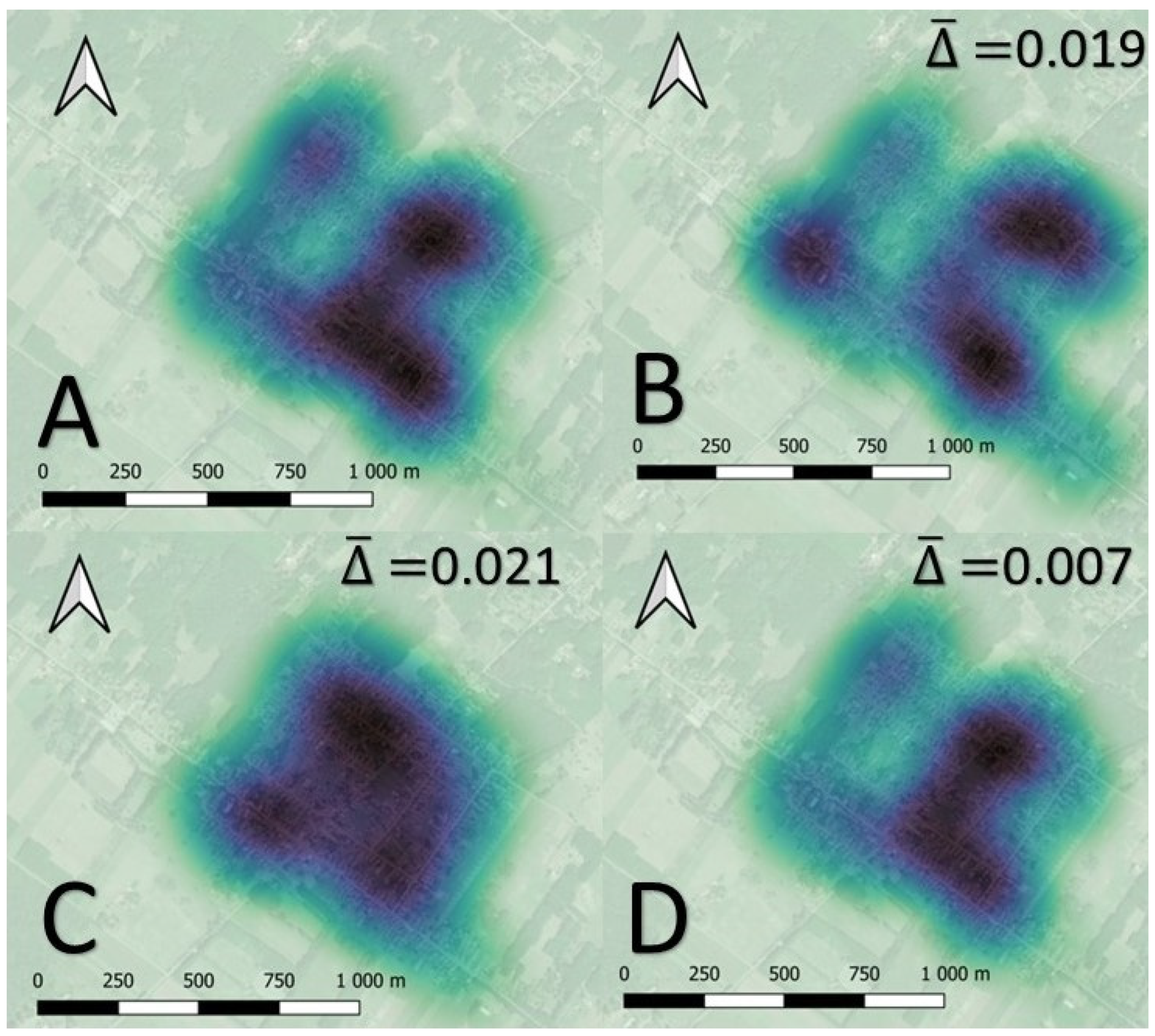
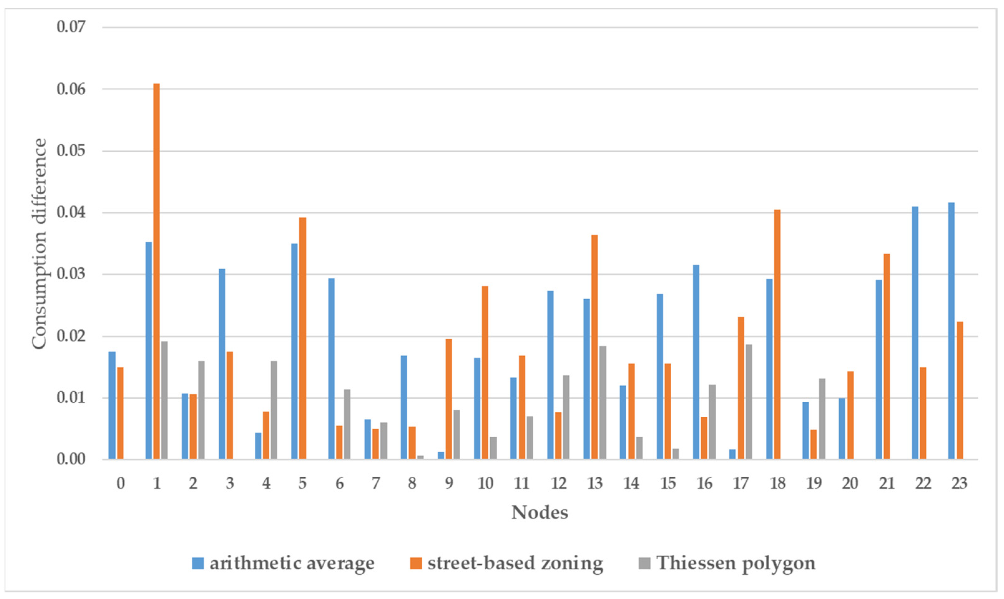
• Effective water consumption allocation may be achieved through delineating the influence range around each node. When contrasting the zoning based on the street approach and the arithmetic average with the benchmark manual range of influence approach, errors of approximately 190% and 230%, respectively, are identified.
• Implementing the manual method becomes excessively time-consuming, especially for larger networks. Consequently, in our study, we have opted for the approach of delineating the influence area using Thiessen polygons. The average disparity between the manual and Thiessen polygon methods is small, a deviation considered quite minimal and within acceptable limits. In municipalities with high-density regions where the water distribution network is dense and consumption points are closely clustered, the manual method may remain preferable due to its ability to account for intricate spatial relationships not captured by automated approaches. Additionally, considering that the construction of new buildings may not always align with the existing water distribution network pipelines, manual intervention may be necessary to ensure accurate representation in such dynamic environments.
• For the future research path, the integration of automation into GIS processes could be outlined such as data collection, analysis, and visualization can be streamlined, leading to more precise and efficient modeling outcomes.

References

1. Marlow, D.R.; Moglia, M.; Cook, S.; Beale, D.J. Towards Sustainable Urban Water Management: A Critical Reassessment. Water Res. 2013, 47, 7150–7161. [Google Scholar] [CrossRef] [PubMed]
2. Pokhrel, S.R.; Chhipi-Shrestha, G.; Hewage, K.; Sadiq, R. Sustainable, Resilient, and Reliable Urban Water Systems: Making the Case for a “One Water” Approach. Environ. Rev. 2022, 30, 10–29. [Google Scholar] [CrossRef]
3. Barton, N.A.; Hallett, S.H.; Jude, S.R. The Challenges of Predicting Pipe Failures in Clean Water Networks: A View from Current Practice. Water Supply 2022, 22, 527–541. [Google Scholar] [CrossRef]
4. Wallace, D.W.; Foster, L.; Schartau, K.; Lewin, D.; Keyes Jr, C.G. Empirical Risk Analysis Methodology for Adversarial Threats against Critical Infrastructure. J. Infrastruct. Syst. 2024, 30, 04023036. [Google Scholar] [CrossRef]
5. Quitana, G.; Molinos-Senante, M.; Chamorro, A. Resilience of Critical Infrastructure to Natural Hazards: A Review Focused on Drinking Water Systems. Int. J. Disaster Risk Reduct. 2020, 48, 101575. [Google Scholar] [CrossRef]
6. Liu, W.; Song, Z. Review of Studies on the Resilience of Urban Critical Infrastructure Networks. Reliab. Eng. Syst. Saf. 2020, 193, 106617. [Google Scholar] [CrossRef]
7. Osei-Kyei, R.; Tam, V.; Ma, M.; Mashiri, F. Critical Review of the Threats Affecting the Building of Critical Infrastructure Resilience. Int. J. Disaster Reduct. 2021, 60, 102316. [Google Scholar] [CrossRef]
8. Fathollahi-Fard, A.M.; Ahmadi, A.; Al-e-Hashem, S.M. Sustainable Closed-Loop Supply Chain Network for an Integrated Water Supply and Wastewater Collection System Under Uncertainty. J. Environ. Manag. 2020, 275, 111277. [Google Scholar] [CrossRef] [PubMed]
9. Larsen, T.A.; Gujer, W. The Concept of Sustainable Urban Water Management. Water Sci. Technol. 1997, 35, 3–10. [Google Scholar] [CrossRef]
10. Bichai, F.; Ryan, H.; Fitzgerald, C.; Williams, K.; Abdelmoteleb, A.; Brotchie, R.; Komatsu, R. Understanding the Role of Alternative Water Supply in an Urban Water Security Strategy: An Analytical Framework for Decision-Making. Urban Water J. 2015, 12, 175–189. [Google Scholar] [CrossRef]
11. Rathnayaka, K.; Malano, H.; Arora, M. Assessment of Sustainability of Urban Water Supply and Demand Management Options: A Comprehensive Approach. Water 2016, 8, 595. [Google Scholar] [CrossRef]
12. Hashemi, S. Sanitation Sustainability Index: A Pilot Approach to Develop a Community-Based Indicator for Evaluating Sustainability of Sanitation Systems. Sustainability 2020, 12, 6937. [Google Scholar] [CrossRef]
13. Mounce, S.R. Data Science Trends and Opportunities for Smart Water Utilities. In ICT for Smart Water Systems: Measurements and Data Science. The Handbook of Environmental Chemistry; Scozzari, A., Mounce, S., Han, D., Soldovieri, F., Solomatine, D., Eds.; Springer: Cham, Switzerland, 2020. [Google Scholar] [CrossRef]
14. Okwori, E.; Pericault, Y.; Ugarelli, R.; Viklander, M.; Hedström, A. Data-Driven Asset Management in Urban Water Pipe Networks: A Proposed Conceptual Framework. J. Hydroinform. 2021, 23, 1014–1029. [Google Scholar] [CrossRef]
15. Okwori, E.; Viklander, M.; Hedström, A. Data Integration in Asset Management of Municipal Pipe Networks in Sweden: Challenges, Gaps, and Potential Drivers. Util. Policy 2024, 86, 101689. [Google Scholar] [CrossRef]
16. Gilbert, T.; James, P.; Smith, L.; Barr, S.; Morley, J. Topological Integration of BIM and Geospatial Water Utility Networks Across the Building Envelope. Comput. Environ. Urban Syst. 2021, 86, 101570. [Google Scholar] [CrossRef]
17. Marzouk, M.; Othman, A. Planning Utility Infrastructure Requirements for Smart Cities Using the Integration Between BIM and GIS. Sustain. Cities and Soc. 2020, 57, 102120. [Google Scholar] [CrossRef]
18. Sharafat, A.; Khan, M.S.; Latif, K.; Tanoli, W.A.; Park, W.; Seo, J. BIM-GIS-Based Integrated Framework for Underground Utility Management System for Earthwork Operations. Appl. Sci. 2021, 11, 5721. [Google Scholar] [CrossRef]
19. Puchol-Salort, P.; O’Keeffe, J.; van Reeuwijk, M.; Mijic, A. An Urban Planning Sustainability Framework: Systems Approach to Blue-Green Urban Design. Sustain. Cities Soc. 2021, 66, 102677. [Google Scholar] [CrossRef]
20. Carriço, N.; Ferreira, B.; Barreira, R.; Antunes, A.; Grueau, C.; Mendes, A.; Covas, D.; Monteiro, L.; Santos, J.; Brito, I.S. Data Integration for Infrastructure Asset Management in Small to Medium-Sized Water Utilities. Water Sci. Technol. 2020, 82, 2737–2744. [Google Scholar] [CrossRef]
21. Gude, V.G.; Muire, P.J. Preparing for Outbreaks–Implications for Resilient Water Utility Operations and Services. Sustain. Cities Soc. 2021, 64, 102558. [Google Scholar] [CrossRef] [PubMed]
22. Berglund, E.Z.; Buchberger, S.; Cunha, M.; Faust, K.M.; Giacomoni, M.; Goharian, E.; Kleiner, Y.; Lee, J.; Ostfeld, A.; Pasha, F.; et al. Effects of the COVID-19 Pandemic on Water Utility Operations and Vulnerability. J. Water Resour. Plan. Manag. 2022, 148, 04022027. [Google Scholar] [CrossRef]
23. Pietrucha-Urbanik, K.; Rak, J. Water, Resources, and Resilience: Insights from Diverse Environmental Studies. Water 2023, 15, 3965. [Google Scholar] [CrossRef]
24. Ezzeldin, R.; Zelenakova, M.; Abd-Elhamid, H.F.; Pietrucha-Urbanik, K.; Elabd, S. Hybrid Optimization Algorithms of Firefly with GA and PSO for the Optimal Design of Water Distribution Networks. Water 2023, 15, 1906. [Google Scholar] [CrossRef]
25. Kruszyński, W.; Dawidowicz, J. Computer Modeling of Water Supply and Sewerage Networks as a Tool in an Integrated Water and Wastewater Management System in Municipal Enterprises. J. Ecol. Eng. 2020, 21, 261–266. [Google Scholar] [CrossRef]
26. Ferraro, A.; Marino, E.; Trancone, G.; Race, M.; Mali, M.; Pontoni, L.; Fabbricino, M.; Spasiano, D.; Fratino, U. Assessment of environmental parameters effect on potentially toxic elements mobility in foreshore sediments to support marine-coastal contamination prediction. Mar. Pollut. Bull. 2023, 194, 115338. [Google Scholar] [CrossRef] [PubMed]
27. Muscetta, M.; Bianco, F.; Trancone, G.; Race, M.; Siciliano, A.; D’Agostino, F.; Sprovieri, M.; Clarizia, L. Washing Bottom Sediment for The Removal of Arsenic from Contaminated Italian Coast. Processes 2023, 11, 902. [Google Scholar] [CrossRef]
28. Fernández Moniz, P.; Almeida, J.S.; Pino, A.T.; Suárez Rivero, J.P. A GIS-Based Solution for Urban Water Management. Water Int. 2020, 45, 660–677. [Google Scholar] [CrossRef]
29. Meijer, D.; Korving, H.; Clemens-Meyer, F. A Topological Characterisation of Looped Drainage Networks. Struct. Infrastruct. Eng. 2022, 1–14. [Google Scholar] [CrossRef]
30. Giudicianni, C.; Di Nardo, A.; Di Natale, M.; Greco, R.; Santonastaso, G.F.; Scala, A. Topological Taxonomy of Water Distribution Networks. Water 2018, 10, 444. [Google Scholar] [CrossRef]
31. Kaltenbacher, S.; Steinberger, M.; Horn, M. Applied Pipe Roughness Identification of Water Networks: Consideration of All Flow Regimes. IEEE Trans. Control Syst. Technol. 2022, 31, 676–691. [Google Scholar] [CrossRef]
32. Yao, L.; Zhang, H.; Zhang, C.; Zhang, W. Driving Effects of Spatial Differences of Water Consumption Based on LMDI Model Construction and Data Description. Cluster Comput. 2019, 22, 6315–6334. [Google Scholar] [CrossRef]
33. Cichoń, T.; Królikowska, J. Remote Reading of Water Meters as an Element of a Smart City Concept. Rocz. Ochr. Srodowiska 2021, 23, 883–890. [Google Scholar] [CrossRef]
34. Trancone, G.; Spasiano, D.; Race, M.; Luongo, V.; Petrella, A.; Pirozzi, F.; Fratino, U.; Piccinni, A.F. A combined system for asbestos-cement waste degradation by dark fermentation and resulting supernatant valorization in anaerobic digestion. Chemosphere 2022, 300, 134500. [Google Scholar] [CrossRef] [PubMed]
35. Cetl, V.; Kliment, T.; Jogun, T. A Comparison of Address Geocoding Techniques—Case Study of the City of Zagreb, Croatia. Surv. Rev. 2018, 50, 97–106. [Google Scholar] [CrossRef]
36. Orgoványi, P. Increasing the Efficiency of Loss Analysis of Public Water Supply Networks Using Geospatial Method. Műszaki Katonai Közlöny 2023, 33, 95–105. (In Hungarian) [Google Scholar] [CrossRef]
37. Bao, Y.; Mays, L.W. Model for Water Distribution System Reliability. J. Hydraul. Eng. 1990, 116, 1119–1137. [Google Scholar] [CrossRef]
38. Gaafar, M.; Mahmoud, S.H.; Gan, T.Y.; Davies, E.G.R. A practical GIS-based hazard assessment framework for water quality in stormwater systems. J. Cleaner Prod. 2020, 245, 118855. [Google Scholar] [CrossRef]
39. Khoa Bui, X.; Marlim, M.S.; Kang, D. Water Network Partitioning into District Metered Areas: A State-Of-The-Art Review. Water 2020, 12, 1002. [Google Scholar] [CrossRef]
40. Kanakoudis, V.; Muhammetoglu, H. Urban Water Pipe Networks Management towards Non-Revenue Water Reduction: Two Case Studies from Greece and Turkey. Clean–Soil Air Water 2014, 42, 880–892. [Google Scholar] [CrossRef]
41. Kawathe, L.N.; Thorvat, A.R. Analysis and Design of Continuous Water Distribution System against Existing Intermittent Distribution System for Selected Area in Pandharpur, MS, India. Aquademia 2020, 4, ep20028. [Google Scholar] [CrossRef] [PubMed]
42. Pudasaini, B.; Shahandashti, M. Seismic Rehabilitation Optimization of Water Pipe Networks Considering Spatial Variabilities of Demand Criticalities and Seismic Ground Motion Intensities. J. Infrastruct. Syst. 2021, 27, 04021028. [Google Scholar] [CrossRef]
43. Mosbach, J.; Sonnenburg, A.; Fiedler, J.E.; Urban, W. Development of a New Method to Support a Participatory Planning for Piped Water Supply Infrastructure in Informal Settlements. Water 2022, 14, 1316. [Google Scholar] [CrossRef]
44. Wright, R.; Stoianov, I.; Parpas, P.; Henderson, K.; King, J. Adaptive Water Distribution Networks with Dynamically Reconfigurable Topology. J. Hydroinform. 2014, 16, 1280–1301. [Google Scholar] [CrossRef]
45. Perelman, L.; Ostfeld, A. Topological Clustering for Water Distribution Systems Analysis. Environ. Model. Softw. 2011, 26, 969–972. [Google Scholar] [CrossRef]
46. Singh, S.K. Evaluating two freely available geocoding tools for geographical inconsistencies and geocoding errors. Open Geospat. Data Softw. Stand. 2017, 2, 11. [Google Scholar] [CrossRef]
47. Chow, T.E.; Dede-Bamfo, N.; Dahal, K.R. Geographic disparity of positional errors and matching rate of residential addresses among geocoding solutions. Ann. GIS 2016, 22, 29–42. [Google Scholar] [CrossRef]
48. Cureau, R.J.; Ghisi, E. Reduction of Potable Water Consumption and Sewage Generation on a City Scale: A Case Study in Brazil. Water 2019, 11, 2351. [Google Scholar] [CrossRef]
Figure 1. Population changes in the investigated settlement between 2000 and 2022.
Urbansci 08 00035 g001
Figure 2. Distribution of permanent population by age and sex.
Urbansci 08 00035 g002
Figure 3. Dwelling types of the investigated municipality.
Urbansci 08 00035 g003
Figure 4. Amount and distribution of the supplied water.
Urbansci 08 00035 g004
Figure 5. Geocoded consumption points (blue triangles).
Urbansci 08 00035 g005
Figure 6. Base network topology. Red squares are the connection nodes.
Urbansci 08 00035 g006
Figure 7. Consumption heat map generated from the results of the arithmetic average method.
Urbansci 08 00035 g007
Figure 8. Zone delineation based on streets. Red squares are the connection nodes, blue triangles are the consumption points.
Urbansci 08 00035 g008
Figure 9. Manual determination of the nodes’ range of influence. Red squares are the connection nodes, blue triangles are the consumption points.
Urbansci 08 00035 g009
Figure 10. Determination of the nodes’ range of influence based on Thiessen polygons. Red squares are the connection nodes, blue triangles are the consumption points.
Urbansci 08 00035 g010
Figure 11. Consumption heat maps based on manual method (A), zoning based on the street (B), arithmetic average (C), and Thiessen polygons (D).
Urbansci 08 00035 g011
Figure 12. Consumption differences at each node in different scenarios.
Urbansci 08 00035 g012
Figure 13. Water demand rate distribution.
Urbansci 08 00035 g013
Disclaimer/Publisher’s Note: The statements, opinions and data contained in all publications are solely those of the individual author(s) and contributor(s) and not of MDPI and/or the editor(s). MDPI and/or the editor(s) disclaim responsibility for any injury to people or property resulting from any ideas, methods, instructions or products referred to in the content.