Abstract
Urban mobility and geographical systems benefit significantly from a graph-based topology. To identify the network’s crucial zones in terms of connectivity or movement across the network, we implemented several centrality metrics on a particular type of spatial network, i.e., a Region Adjacency graph, using three geographical regions of different sizes to exhibit the scalability of conventional metrics. To boost the topological analysis of a network with geographical data, we discuss the eigendata centrality and implement it for the largest of our Region Adjacency graphs using available geographical information. For flow prediction data-driven models, we discuss the Deep Gravity model and utilise either its geographical input data or predicted flow values to implement an additional node score through the Perron vector of the transition probability matrix. The results show that the topological analysis of a spatial network can be significantly enhanced by including regional and mobility data for graphs of different scales, connectivity, and orientation properties.
1. Introduction
The application of topology to geographic structures has revealed new insights into spatial dynamics [1]. Topological analysis of networks associated with urban, mobility, and geographical structures is useful to identify critical spots in the network. These spots can be interpreted as relevant zones that make transit across the network more difficult or leave some of the zones disconnected. In addition, these failures have safety and economic repercussions. Network structure can be analysed using different concepts, with centrality being the most important one [2]. Node centrality metrics measure the relevance of a node in a graph according to topological criteria. For example, the betweenness centrality can serve as an indicator of the vulnerability to traffic interruption of a station in an underground network [3,4], and the closeness centrality can be used to identify the stations with better connections in a network in the context of reducing overall distance, travel time, or related road factors.
The insights obtained from node centrality metrics can be boosted if additional external information on the nodes is available. This is the case for urban mobility and geographic networks, where collections of geo-located data about buildings, lands, and cities are becoming a rich source of information. Some additional node metrics have been defined combining the idea of a conventional centrality metric and the implementation of geo-referenced data, e.g., the eigendata centrality [2] has been used to find relevant roads in a city taking into account the topology of the road network and the existence of various points of interest across the city.
Regarding the latest advancements in traffic and mobility data-driven modelling, we identify two main frameworks: Euclidean models [5,6], which apply grid partitions over an area of interest to intra-regional flow forecasting, and non-Euclidean models [7,8], which apply graph-based structures. They are better suited and more reasonable for mobility modelling, as spatial dependencies do not always occur between adjacent cells in a grid partition. Flow prediction models, e.g., the Deep Gravity model [9], have been enhanced by considering the effect of geographical data. The Deep Gravity model is a Deep Learning approach that generalises the singly constrained gravity model for flow forecasting by not including only the population as a factor for mobility flows between regions but also including several geographical features (e.g., land use, transport, food, and health facilities) available for them. This model allows us to perform additional centrality evaluations on an area where mobility flows are known or generated. By examining mobility flow alongside the network structure, we gain a clearer insight of how the network configuration influences flow dynamics, with other contributing elements like operational adjustments and seasonal variations that have an impact on travel patterns.
As an overall goal, we aim to present a variety of methods for analysing and visualising information that have the potential to enhance the dynamics forecast provided by data-driven traffic and mobility models. To this end, we review existing data-driven models for flow prediction (Section 2) using either Euclidean-based or non-Euclidean-based approaches, emphasising the characteristics of the Deep Gravity mobility model. We introduce basic concepts of Graph Theory (Section 3), such as connectivity, directionality, and degree and transition probability matrices, which allow us to define node centrality metrics for both undirected and directed graphs. Indeed, we compare several definitions of Graph Laplacian matrices (e.g., the Combinatorial Laplacian, the Symmetrised Laplacian, the Diplacian); some of them are based on the Perron vector. We discuss how the Perron vector has the potential to be used to define node scores through the so-called circulation functions. Additionally, we discuss how the eigenvector centrality has been adjusted for spatial networks when geographical data are available. We compute the conventional centrality metrics for a particular class of spatial graphs, i.e., the Region Adjacency graph (Section 4) is generated by partitioning a geographical region into sub-regions, identifying graph nodes with sub-regions and encoding neighbouring sub-regions as graph edges.
We use concepts, such as the transition probability matrix and its Perron vector, to review the concept of circulation functions that can be particularly meaningful for networks related to flows and mobility. We perform a novel geographical feature-based centrality analysis for a region where the Deep Gravity model has been implemented. This is a relevant approach to address the need for merged analysis using node centrality metrics based on geographical features, and mobility flows based on geographical networks, as the Deep Gravity model predicted. The predicted flows were used as the edge weights to construct a circulation function.
For the experimental tests, we consider three Region Adjacency graphs: Genova Province, the United Kingdom, and New York State, using the Earth distance between the centroids of two zones defined through the Haversine formula as edge weights. Computing and interpreting several node centrality metrics on geographical networks of different sizes, we demonstrate the adaptability and scalability of these tools for the topological analysis of networks embedded into a two-dimensional space. Given the availability of the geographical input features of the Deep Gravity model and its predicted flows for New York State, on this Region Adjacency graph, we additionally compute the eigendata centrality and implement a circulation function based on the Perron vector of the transition probability matrix using the predicted flows as edge weights. Then, we proceed to discuss the results from the tests (Section 5). We draw various conclusions (Section 6) and indicate the possible extent of this work.
2. Previous Work
Graph-based approaches equip models with several theoretical elements for analysing and interpreting complex networks. By defining a value or score on a graph node, we can measure its importance or impact within the network. Network robustness can be defined as the ability of a network to maintain its function under challenges or failures [10]. Such failures are often referred to as the eventual removal of some nodes and their incident edges. This property is known as network resilience and is measured through an assessment of the most significant component after the failures [11]. Different types of centrality metrics have been applied to assess the robustness of a network and to find nodes with various levels of importance, particularly in urban and mobility networks. The betweenness centrality has been applied to identify metro stations and roads with the potential to become a point of congestion or to affect the rest of the system during some interruption or failure [3], and as a statistical analysis tool to find the roads that are potential traffic congestion points in the Indian highway network [4]. Because of the nature of urban and transport networks, the spatial topology often does not contain all the information of the nodes. The eigendata centrality is a node centrality score considering the city’s geographical features (e.g., land use, transport, food, and health facilities) to find relevant zones.
Using weights on the edges of a graph allows us to represent additional features in mobility models, e.g., the road length, the road capacity, or some geographical features associated with the studied region. The betweenness centrality has been used on dynamically weighted graphs [12] to discover correlations between centrality metrics and mobility data, allowing us to consider factors external to the network topology when evaluating the importance of a node. Relevant nodes have been identified in urban and geographical networks. Metrics that include information of a zone modelled as a node have been implemented to consider the effect of external factors on the network topology, e.g., the eigendata centrality [2] has been used to find influential zones within a city using a modified version of the eigenvector centrality that takes into account the distribution of different points of interest in the town. In addition to scoring the zones of a region partition, another problem studied was the estimation of flows between different zones. It is natural to expect that there are not only spatial factors (topology) but external factors (geography) that motivate the mobility of individuals, as well as mobility inflows and outflows in each zone.
Flow forecasting models employ various kinds of mobility data and prediction approaches. Euclidean methods (or grid-based methods) partition an area of interest into a square or rectangular grid to assess the number of displacements between adjacent cells. In contrast, non-Euclidean methods (or graph-based methods) use graphs that can be constructed using distinct approaches, e.g., considering transport stations or monitoring sensors as nodes where the edges represent the dissemination paths of the data or defining the nodes on non-overlapping sub-areas where the edges represent the existence of a common border, as with the Region Adjacency graphs. The data flow from one node to another may exist even if they are not geographically close as in the regular grids. When dividing the city into a grid, urban flows, traffic volumes, and other mobility data can be represented in matrices or tensors, depending on the number of available mobility variables, while when working with graphs, all these types of data are stored as graph signals. In addition to the domain’s topology and mobility-related data, external factors impact mobility, e.g., weather conditions, special events, and points of interest.
Despite applications of grid-based models to traffic forecasting, some aspects suggest that modelling mobility in a city as a graph is convenient. For instance, the structure of road networks can be considered a graph topology that connects different locations in a geographic region, i.e., graph nodes, and the associated mobility information between any couple of connected sub-regions can be considered graph weights. Due to its geographical nature, urban road networks are a standard example of a spatial network [13,14] and, typically, adjacent cells in the grid do not experience flows between them during certain periods because they are not connected by direct roads. In [14], various strategies are introduced for constructing graph-based models, incorporating distinct mobility data sets and Deep Learning methods.
Large amounts of information have allowed the implementation of several data-driven models, mainly using Deep Learning techniques. In addition to the spatial data, grid-based models can also considers different types of temporal dependencies, i.e., close past time intervals, periods of the year, or trends in the last hours or weeks. The ST-ResNet model [5] and the STRN model [6] are instances of spatio-temporal models. They use data sets with trajectories of cars, bicycles, and people. The difference between both methods mainly consists of the granularity level in which the city is partitioned. In the graph-based models, the spatial part has greater weight since different weights on the links of the network will result in stronger or weaker connections between the partitioned areas, which can model the spatial dependencies from alternative approaches, e.g., the ETGCN model [7] and the GTA model [8] use data collected by sensors (the nodes) distributed over the roads of a city; the former consider three types of weights to obtain a merged value that takes into account different kinds of information, while the latter uses the distances between the sensors as the weight of the links. With this type of graph, vehicle flow can be predicted, and average speeds and other traffic variables can be expected.
The Deep Gravity model [9] applies a grid-based approach as an initial step to classify training and testing areas and then uses a secondary irregular partition to perform flow forecasting. The name of this model comes from Newton’s law of universal gravitation and its Deep Learning approach. In mobility gravity models, the flow from zone i to zone j is expected to be proportional to the population in each zone and inversely proportional to the distance between them. In particular, the singly constrained gravity model estimates the flow from i to j through , where is the distance between them; is the population in each of the zones, and is a real parameter. The deterrence function f can be exponential or a power-law function. The singly constrained gravity model requires the availability of the total outflows . The fraction that multiplies is a value in that represents the probability of a movement from one zone to another or the proportion of the outflows from i to each destination zone.
The Deep Gravity model is a generalisation of the singly constrained gravity model to a feed-forward neural network to estimate the probability of observing a flow from an irregular element i of the region partition to another irregular element j inside the same cell of the initial grid-based partition. Thus, the predicted flows are limited only to locations within the same regular cell, which, from the Graph Theory point of view, means that if one expects to use the flows to construct the weights of the edges, the lack of values for some links will result in disjointed graph components. In addition to the population, the Deep Gravity model considers eighteen geographical features for each irregular location, e.g., land-use areas, road network information, transport, food, education, and retail facilities. The Deep Gravity model relies on population data taken from official census sources and geographic attributes collected from OpenStreetMap.
The analysis of static node importance in mobility networks has been previously studied in terms of connectivity and vulnerability, e.g., on underground metro systems [3], which are naturally related to mobility flows. Also, the dynamic vulnerability of networks based on passenger demand has been addressed for urban rail transit systems [15] where the relevance of a node evolves in time. This demonstrates the relevance of a combined study between mobility flows and network vulnerabilities, in particular for mobility networks without physical infrastructure, e.g., networks for intra-regional mobility. Mobility prediction approaches, such as the Deep Gravity model, provide us with essential elements to investigate the combination of the two problems, namely, the mobility flows between irregular zones of a region partition and the involvement of geographical features.
3. Standard and Spatial Graphs: Definitions and Metrics
We present elementary concepts from Graph Theory that are crucial for network-based models (Section 3.1); then, we discuss standard centrality metrics that are suitable for topological analysis of networks (Section 3.2), as well as Graph Laplacian matrices (Section 3.3) and additional node scores based on geographical features (Section 3.4) that enhance the analysis of spatial networks.
3.1. Graphs’ General Concepts
A graph is defined through a node set and an adjacency matrix with non-negative entries (weights) that satisfy if and only if there is an edge between node i and node j. Such connections represent a relationship between the nodes or a flow from one to another. If the adjacency matrix is symmetric, then the graph is called undirected because and represent the same link. If the adjacency matrix is not symmetric, then the graph is called directed because there is an orientation within the graph.
Paths and distances: A path w (or a walk) [16] on a graph is a sequence of nodes where is an edge of the graph and for . The length of w is defined by . Given two nodes , a shortest path from a to b is a path such that , , and there is no path from a to b with a smaller length. The distance from a to b is the length of the shortest path from a to b. If there is no path from a to b, we define its distance as infinity. Moreover, the distance from a node to itself is defined as zero.
Connected components: A graph is connected (when the graph is undirected) or strongly connected (when the graph is directed) if for every pair of nodes there exists a path from i to j. Otherwise, it is disconnected. A directed graph is called weakly connected if its underlying undirected graph is connected. A disconnected graph can be decomposed into smaller connected sub-graphs called connected components.
Degree and transition probability matrices: The In-Degree Matrix and the Out-Degree Matrix are the diagonal matrices and with diagonal entries defined as and , respectively. If the graph is undirected, the In-Degree and the Out-Degree Matrices are the same.
Transition probability matrix and Perron vector: From this point onwards, we use the notation to refer to the Out-Degree Matrix regardless of the directionality of the graph. We define the transition probability matrix of the Markov chain associated with random walks on the nodes of the graph [17] as , provided that there are no nodes (called dead-end nodes) without outgoing edges. The matrix is called the normalised adjacency matrix of the graph [18]. The transition probability matrix is stochastic, i.e., all its entries are non-negative, and the sum of each row is 1, i.e.,
for every . The entry represents the probability of moving from node i to j or the proportion of the flow moving from i to j. For a strongly connected directed graph, the Perron–Frobenius theorem guarantees the existence of a unique left eigenvector with positive components for the transition probability matrix, i.e., . The vector is called the Perron vector of , and it can be proven that . We normalise the entries of such that .
3.2. Centrality Metrics for Nodes
The simplest score we can assign to a node is obtained through the diagonal elements of the degree matrices. The In-Degree Centrality and the Out-Degree Centrality of a node v are defined by and , where and are the In-Degree and the Out-Degree Matrices, respectively. The node’s In-Degree and Out-Degree can be interpreted as a weighted number of inflows or outflows through that node. The In-Degree and the Out-Degree Centralities of a node in an undirected graph are the same value, and it is just called Degree Centrality.
A connected graph represents the possibility of choosing any node as a starting point and arriving at any other one within the network following some paths; some nodes will require larger distances than others. The In-Closeness Centrality and the Out-Closeness Centrality are defined by
respectively. Both are the inverse of average distances between i and the rest of the nodes. A node with smaller distances to the rest of the network has a smaller average distance and, consequently, the highest closeness centrality. In contrast, a node with a larger average distance to the rest of the network has a smaller closeness centrality because it requires longer paths to connect with the other nodes. The In-Closeness and the Out-Closeness of a node in a directed graph take into account the direction of the edges, and they represent the ease of being reached from the rest of the network or reaching the rest of the network, respectively. The In-Closeness and the Out-Closeness centrality of a node in an undirected graph are the same value, called Closeness Centrality.
Closeness centralities are inconvenient with disconnected graphs. Indeed, for every node i, there exists another node j without either a path starting on i and ending on j or a path from j to i. Thus, or , meaning that or for every node. Alternative scores that take into account the idea of average distances among the nodes that are meaningful even for disconnected graphs are the In-Harmonic Centrality and the Out-Harmonic Centrality, which are defined by
respectively. They are the average of the inverse distances from a node to the rest of the network; in this way, the contribution of the disconnected nodes is excluded because it simply vanishes.
Similar to closeness centrality, a node with smaller distances from the other nodes will have larger harmonic centrality. In comparison, a node with larger distances to the rest of the network will have smaller Harmonic Centrality values and and for every (we apply the inequality ). A node of a directed graph will have a zero In-Harmonic or Out-Harmonic Centrality value if and only if its In-Degree or Out-Degree, respectively, is zero. The In-Harmonic and Out-Harmonic Centralities of a node in an undirected graph are the same value, called Harmonic Centrality. For the shortest paths between every pair of nodes, there exist some nodes that belong to a larger number of paths, representing a higher importance as a “bridge” between other pairs of nodes since it helps to create the shortest path between them and their removal may represent an incremental value of their total distance. A score to assess such linking importance is the betweenness centrality, which is defined by , where denotes the number of shortest paths from a to b and, by convention, for every node i [19]. The value denotes the number of shortest paths from a to b with i as an intermediate node. The betweenness centrality quantifies the extent to which a node serves as a bridge between others in a graph. It calculates the ratio of shortest paths between any two nodes that go through the node in question. The greater the betweenness centrality, the more frequently the node is part of these shortest routes. Nodes with high betweenness centrality are critical for maintaining network integrity. Removing such a node could compromise the graph by eliminating optimal routes or completely isolating certain nodes from the network. A node will have a betweenness centrality of zero if it is not traversed by any shortest paths between other node pairs.
On directed graphs, another score is the influence a node has depending on the influence of its incoming neighbours. If a node is connected to an influential node, its own influence in the graph will intuitively be stronger than if it were connected to a less influential node. The PageRank centrality of a node i [20] is defined in a recursive way through
where the are the nodes such that there is an edge from to i, for . Moreover, the value is called the damping factor and is usually set to ; it is a trade-off between the influence of the incoming neighbours and the influence of some external factors. The PageRank values are computed as the principal eigenvector of the matrix [21], i.e., the right eigenvector whose eigenvalue has the largest magnitude, where is defined as . The matrix is the transition probability matrix; is a distribution probability called the teleportation vector, whose component i denotes the probability to arrive at the node i during a random walk along the directed edges of the graph; and is the Kronecker delta vector with components for and .
Another approach to measuring the influence or popularity of a node in a network from the importance of its connections is using direct proportionality, i.e., assuming that the centrality value at node i is proportional to the weighted average of the centralities of its neighbours: . This relation can be written in matrix form as , i.e., is a right eigenvector of the adjacency matrix . A centrality metric for a node is expected to be non-negative and well defined. If represents a connected undirected graph or a strongly connected directed graph, the Perron–Frobenius theorem guarantees the existence of a unique right eigenvector with non-negative entries and can be defined as the Eigenvector Centrality [22]; this eigenvector is furthermore associated with the eigenvalue with the largest magnitude among all the eigenvalues. Since it is a right eigenvector, the eigenvector centrality measures the influence of a node i by weighting the influence of its outgoing neighbours. In a directed graph, the nodes with a zero eigenvector centrality value are those with zero Out-Degree and those whose only outgoing neighbours have zero influence. The nodes with a zero eigenvector centrality score are isolated in an undirected graph. The standard centrality metrics are outlined in Table 1.

Table 1.
Summary of centrality metrics for the nodes of a graph.
3.3. Graph Laplacian Matrices
The Out-Degree, the In-Degree, and the transition probability matrices measure different levels of importance for the nodes in a graph. The Graph Laplacian matrix and its eigenvalues are important for systems modelled by a graph, as they can explain the graph’s connectivity and support Graph Signal Processing. We introduce the Combinatorial Laplacian for undirected graphs (Section 3.3.1) that have non-negative real eigenvalues and a normalised variation that furthermore has an upper bound for them. Additionally, we present various alternatives for defining the Graph Laplacian for directed graphs (Section 3.3.2) that preserve the real nature of the eigenvalues in most of the cases and some theoretical equivalences between them.
3.3.1. Laplacians of Undirected Graphs
For undirected graphs, we define the Combinatorial Laplacian [18] as . Since the adjacency matrix of an undirected graph is symmetric, the Combinatorial Laplacian is symmetric, and its eigenvalues are real. Moreover, is positive semidefinite. The eigenvalues are positive, and it is possible to define a pseudo scalar product in by letting . The expression is called the Quadratic Laplacian Form. The Combinatorial Laplacian is called the Kirchhoff Matrix of the graph [23].
To obtain a Laplacian matrix whose eigenvalues are contained in the interval regardless of the network structure, we can define the Normalised Graph Laplacian [24] as , where is the identity matrix of dimension N. The Normalised Graph Laplacian of an undirected graph is symmetric, and it is positive semidefinite since is an invertible diagonal matrix with positive entries. Furthermore, the Combinatorial Laplacian and the Normalised Graph Laplacian are related by . For further details on the bounds of the Laplacian eigenvalues, we refer the reader to [25].
3.3.2. Laplacians of Directed Graphs
The symmetry of the Laplacian matrices of undirected graphs is lost for directed graphs because the adjacency matrix is not necessarily symmetric. A definition that keeps symmetry for directed graphs is the Combinatorial Directed Laplacian [26] defined through
The Combinatorial Directed Laplacian is symmetric regardless of the directionality of the graph. It is positive semidefinite since it can be seen as the Combinatorial Laplacian of an undirected graph with adjacency matrix .
We use the Perron vector of the transition probability matrix to define a Laplacian matrix for strongly connected directed graphs. The Symmetrised Laplacian and the Combinatorial Symmetrised Laplacian [16] are defined as
respectively, where = . Here, and are symmetric. Moreover, is positive semidefinite since it can be written as the Combinatorial Laplacian of an undirected graph with adjacency matrix . The Symmetrised Laplacian is positive semidefinite because of the relation and because is a diagonal matrix with positive entries.
The Symmetrised Laplacian and the Combinatorial Symmetrised Laplacian depend on the Perron vector of the transition probability matrix; in consequence, they do not capture the unique characteristic of random walks on directed graphs since different graphs can have the same . An alternative to overcome this matter is to use the Diplacian [17], which is defined as , which is not always symmetric, and in general may have eigenvalues with imaginary parts different from zero.
3.3.3. Properties
The Laplacian matrix is a foundational operator in network models, and it is essential to enable spectral methods, including Graph Signal Processing. The desired properties of the Laplacian matrix are real eigenvalues and positive semidefinite. The directionality of graphs raises the need to define different types of Laplacian matrices that satisfy the desired properties. Certain matrices, like the Combinatorial Directed Laplacian, the Symmetrised Laplacian, and the Combinatorial Symmetrised Laplacian, are always symmetric, regardless of whether the graph is directed or undirected. Furthermore, these Laplacians are positive semidefinite operators because they can be viewed as the Combinatorial Laplacian of an undirected graph with a suitable adjacency matrix, allowing them to inherit the positive semidefinite property of . We examine the key properties of various graph Laplacian matrices and present them in Table 2.
Table 2.
Summary of the properties of different Laplacians.
There are some equivalences between the different types of Laplacian matrices. If the graph is undirected, then , and the Combinatorial Symmetrised Laplacian coincides with the Combinatorial Laplacian.
This symmetry implies self-adjointness with respect to the Euclidean inner product; indeed, if , then if and only if , i.e., . Since is positive semidefinite, then the Normalised Laplacian is positive semidefinite because it can be written as .
The positive semidefiniteness of the Laplacian matrix of a directed graph can be proved by writing it as the Combinatorial Laplacian of an undirected graph, namely, by constructing an adjacency matrix that depends on and obtaining the corresponding degree matrix . For instance, for the Combinatorial Directed Laplacian we can set and , which satisfies that the sum of the i-th row equals . Similarly, for the Combinatorial Symmetrised Laplacian we have that and . The sum of the i-th row of equals ; in fact,
since is row stochastic, and by definition the Perron vector satisfies the relation . The positive semidefinite property for the Symmetrised Laplacian follows from the relation . Graph Laplacians for directed graphs, with the exception of the Diplacian, are typically symmetric. As a result, their eigenvalues are real, and for the Symmetrised and Combinatorial Symmetrised Laplacians, these eigenvalues are bounded.
The Diplacian of a directed graph is symmetric if and only if its adjacency matrix is symmetric. Indeed, we have . Assuming , then . Recalling that , and are diagonal matrices, using their multiplication commutativity, and multiplying by from the left and the right, we obtain . Since and have an inverse, we obtain as a necessary condition for the symmetry of the Diplacian. Conversely, if then is symmetric. If is symmetric, then the Diplacian reduces to , i.e., the Normalised Laplacian.
3.4. Feature-Based Scores for Nodes in Spatial Networks
Within the range of systems modelled by a network, there are some of them where topology alone does not include all the information, and a space or metric notion plays a crucial role in their characterisation. These networks are usually embedded in a two-dimensional or three-dimensional space, e.g., road networks, phone networks, transportation networks, and mobility networks. A Spatial Network is a network with nodes in a space equipped with a metric [27]. The metric for networks in is usually the Euclidean distance. For nodes represented by geographical positions (longitude, longitude) on Earth, the metric can be what we will call the Earth distance, i.e., the distance between the nodes and that is computed through the Haversine formula [28] , where r represents the radius of Earth and can be set as . The Earth distance represents the shortest arc length of the maximum circumference traced on Earth’s surface that passes through two given points (Figure 1).
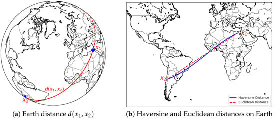
Figure 1.
Earth distance between and (a). The Haversine formula computes the smallest of the two arc lengths of the maximum circumference that passes through and and varies from the Euclidean distance due to the curvature of the Earth (b).
Geographical networks can be constructed from the spatial partitioning of a region into non-overlapping sub-regions. Two elements from a partition of a geographical area are called neighbours if they are spatially adjacent, i.e., if they share borders larger than zero meters [29]. The Region Adjacency graph (Figure 2) induced by a region is a graph that uses the elements of its partition as nodes with edges indicating that the sub-regions i and j are neighbours. The binary adjacency matrix of a Region Adjacency graph with weights in is known as a spatial adjacency matrix. Furthermore, the sub-regions may have additional relationships even if they are not neighbours; for instance, they can represent mobility information from one sub-region to another, commerce routes, people’s commuting habits, or some relationship between some regional communities. This additional data can be stored in a matrix , which can be used to construct a weighted adjacency matrix for the Region Adjacency graph by using the Hadamard element-wise product , i.e., . Mobility information between the sub-partitions of a region can be stored in an Origin-Destination (OD) Matrix where represents some movement counting or volume flow from i to j. An OD Matrix is not necessarily symmetric.
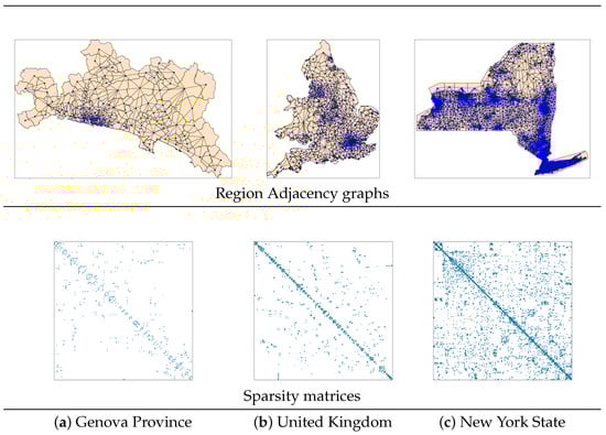
Figure 2.
Region Adjacency graphs and sparse adjacency matrices. (a) Genova Province (GOA Province) partitioned into 137 zones; (b) United Kingdom (UK) partitioned into 344 local authority districts; (c) New York State (NY State) partitioned into 5410 census tracts.
The centrality metrics for spatial networks only consider the graph’s topology, and they do not incorporate any spatial data not represented by the weights of the adjacency matrix that might be available for the network’s nodes. Large amounts of information can be obtained for urban and geographical networks, e.g., information on roads and streets, population, and the distribution of buildings and land types. Reference [2] proposes an eigenvector-based centrality that incorporates information from the topology and the data residing on the nodes. Assuming the existence of data types, we can construct a matrix called the data matrix, where the entry represents the value of the feature j at node i. To combine the data types into a single value for each node, we define the weight vector , whose values are in the range . A vector with every component equal to 1 means all the features have the same importance. The data vector is then defined as and is normalised as . The data adjacency matrix is then defined as , where is the matrix with 1 in every entry, is the importance matrix with entries whenever , and ∘ is the Hadamard element-wise multiplication. The parameters are intended to add a small basic level of importance associated with all the edges and to regularise the eigenvector of associated with the eigenvalue with the largest magnitude. They are chosen as and . If is the eigenvector of associated with the eigenvalue with the largest magnitude, the Eigendata Centrality of i [2] is defined by , where is the eigenvalue associated with . Adding is to spread the importance of neighbouring nodes in the network.
Another approach to add scores to a node is by aggregating some associated values defined on its incident edges, for instance, through a circulation function defined on the edges of a graph, which is a non-negative real-valued function that satisfies , for every i, i.e., the sum of the values on the incoming edges equals the sum of the values on the outgoing edges for every node, providing the idea of some flow preservation. For example, the weights of the adjacency matrix of an undirected graph represent the values of a circulation function defined on the edges. Moreover, a circulation is said to be invertible if for every pair of nodes .
For a connected undirected graph or a strongly connected directed graph, we can use the Perron vector of the transition probability matrix to define a circulation function, namely . For undirected graphs, is invertible. We can now define the Average Perron node circulation at a node i as . The quotient to obtain the circulation per weighted number of connections was performed with since the transition probability matrix was defined using the Out-Degree Matrix. The property that defines a circulation function represents some flow of information through the preserved nodes, and computing the average value at a node measures a weighted velocity at which the information is passing through that node. For the Perron circulation, the average value on the nodes simplifies to .
4. Graph Theory for Spatial and Mobility Data: Experimental Results
Region Adjacency graphs are a network structure that can be leveraged in urban mobility and geographical modelling. We compute and interpret the conventional centrality metrics on three Region Adjacency graphs of different sizes, using the Earth distance as the edge weights (Section 4.1). In addition, the availability of geographical and mobility data from the Deep Gravity model is applied to implement the eigendata centrality on the largest of the graphs (Section 4.2) and to compute the Average Perron node circulation using the ground truth and the predicted flow values. We visualise the eigenvectors of different Laplacian matrices associated with the eigenvalues with the smallest magnitudes (Section 4.3) for our Region Adjacency graph with fewer nodes.
4.1. Node Centrality Metrics in Region Adjacency Graphs
We define the Region Adjacency graphs for three different regions: Genova Province partitioned into zones consisting of 137 nodes and 333 edges, the United Kingdom partitioned into census tracts composed of 343 nodes and 836 edges, and New York State partitioned into output areas consisting of 5410 nodes and 14,842 edges. We embed each node of these graphs in a two-dimensional space by considering the longitude and latitude of their centroids. The three graphs are undirected, connected, and highly sparse because most sub-regions have only a few neighbours. In some cases, clusters of sub-regions can emerge, causing node agglomerations that are evident along the diagonal of the graph’s sparsity matrix (Figure 2).
To each Region Adjacency graph, we associate a weight matrix where the entry represents the Earth distance between the sub-region i and the sub-region j. Using the corresponding spatial adjacency matrix , we can construct a weighted adjacency matrix . We compute the main centrality metrics for the three Region Adjacency graphs (Figure 3) using the weighted adjacency matrix and normalise the values for homogeneity (Figure 4).
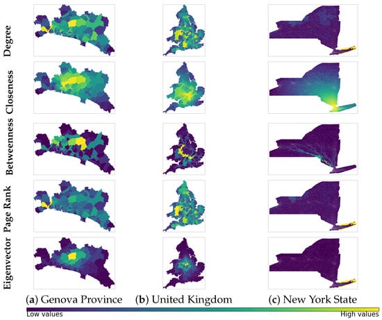
Figure 3.
Centrality metrics for the nodes of Region Adjacency graphs using the Earth distance between contiguous sub-regions as the weight of the edges. Given that the variability of values ranges for each centrality and graph, a qualitative colour bar was adopted.
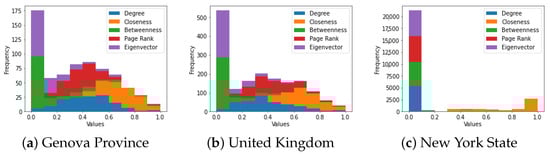
Figure 4.
Distribution of normalised centrality metrics for the Region Adjacency graphs with Earth distances as weights in the adjacency matrix.
The normalised values of the degree centrality for the nodes on the Genova Province and United Kingdom graphs show nearly symmetric behaviour with respect to their mode ( and , respectively) with a clustering of values around them. This explains why we can observe the existence of only a few sub-regions with low and high scores, while most of the sub-regions have intermediate centrality values. In contrast, most of these values are close to for the New York State graph, which explains why we can observe very low scores for most sub-regions. Because of the granularity of the partition for New York State, the distances between neighbours are shorter, and the sub-region with the highest score holds this property because it has many neighbours with a significant aggregated distance.
The normalisation of the closeness centrality shows similar behaviour for the three Region Adjacency graphs: a clustering of values around the high scores and almost no frequencies for the low values. This can be visualised as a portion of the region with the highest scores, progressively decreasing to the rest of the sub-regions, with only a few low scores. Moreover, since we are using the Earth distance as the weights of the edges, the sub-regions with the highest closeness centrality values are the ones from which we can reach the rest of the network with less total distance moving along maximal circles along Earth; this is why it is meaningful that there is a cluster of sub-regions with the highest scores because a close neighbour of the sub-region with the highest accessibility to the rest of the network should have a high degree of accessibility.
The normalised betweenness centrality values are low for the three graphs, particularly in New York State. This explains why we can visualise more sub-regions with high Genova and United Kingdom scores. The sub-regions with higher scores will be more transited during journeys within the whole region when the minimisation of the geodesical distance is pursued. Moreover, the path pattern represents the existence of some optimal routes or trajectories. There are more such optimal routes for Genova and the United Kingdom than for New York State; this suggests that nodes in networks of larger size may use similar routes when optimising distances during journeys within the network.
Most of the normalised eigenvector centrality values are low, close to , for the three graphs. Particularly for New York State, there is only one sub-region with noticeably large scores that coincide with the sub-region with the highest degree of centrality. The Genova Province and the United Kingdom graphs show some sub-regions with intermediate scores clustered around the highest value, which still coincides with the cluster of sub-regions around the one with the highest degree of centrality. This correlation between the highest values of eigenvector centrality and degree centrality is one of the reasons for the implementation of additional node scores for spatial networks that take into consideration the geographical information of the nodes [2]. The normalised values of the Page rank centrality show more variability than the eigenvector centrality, but some correlation with the degree centrality values is still visible. This suggests that using the eigenvector and the Page rank centralities on Region Adjacency graphs to find influential or relevant nodes might be misleading when additional geographical information is not considered.
4.2. Eigendata Centrality from Geographical Features and Mobility Flows
With the weighted adjacency matrix using the Earth distance as edge weights and available geographical information on the sub-regions, we can construct the eigendata centrality. We use the 18 geographical features considered in the Deep Gravity model; to each feature, we assign the same level of importance by imposing a weight vector . We set . The sub-regions with the highest eigencentrality scores are not related to the ones with the highest degree of centrality, as was the case with the standard eigenvector centrality. Now, the cluster of the highest values is located around the sub-regions with the highest normalised data vector values (Figure 5). Because node scores measure the influence or relevance of a node based on its neighbours, the eigendata centrality, as well as the Page rank and the standard eigenvector centrality, produces a hub of nodes with the highest levels of influence or relevance, and suddenly decreases to the rest of the nodes, suggesting that the property of being influential or relevant is reserved for a small connected group of nodes. The eigendata centrality shows some diffusivity from the node with the highest score instead of rapidly decreasing, as with the standard eigenvector centrality, which is stated in [2] and is consistent with the idea that when existing geographical information is linked to a node, both the node itself and its neighbouring nodes have influential results.
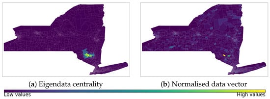
Figure 5.
Eigendata centrality for the New York State Region Adjacency graph with the Earth distance between neighbour sub-regions as edge weights. The cluster of sub-regions with the highest eigendata scores is located around the sub-regions with the highest values on the normalised geographical data vector.
We now consider the weighted adjacency matrix where is an Origin-Destination Matrix to construct mobility flow-based scoring for the nodes on the New York State graph. We evaluate two cases: the ground truth Origin-Destination flows used by the Deep Gravity model and its predicted values. Furthermore, since the Deep Gravity model provides flows within different disjointed subsets of the partition, we will substitute every with to consider minimum flows in the two directions between every pair of neighbour sub-regions, and to guarantee that the weighted adjacency matrix represents a strongly connected directed graph. The Perron vector of the associated transition probability matrix can be used to define the Average Perron node circulation at every node. The distribution of the scores of the Average Perron node circulation is very similar for both the real and the predicted Origin-Destination flows (Figure 6).
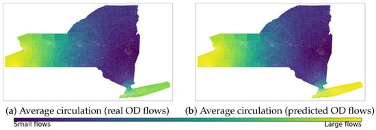
Figure 6.
Average Perron node circulation values for the geographical partitions associated with the New York State Region Adjacency graph. The graph weights are the ground truth (a) and the forecast (b) OD flow values using the Deep Gravity model. Since the OD flows are not symmetric, the graph is directed. It is strongly connected because of the minimum flow term.
4.3. Node Scoring from the Eigenvectors of Laplacian Matrices
Both the eigenvector and the eigendata centralities are based on the eigenvector of a matrix related to the graph’s topology, with some dependence on the adjacency matrix. The novelty of eigendata centrality is that it includes geographical features. This inclusion helps mitigate its localised effect on a subset of nodes of the eigenvector centrality values.
We compute the eigenvectors associated with the eigenvalues with the second, third, and fourth smallest magnitudes of several Graph Laplacian matrices for the Region Adjacency graph of Genova Province. We observe that they show a diffusion behaviour similar to the one of the closeness centrality, but with the highest values on the external sub-regions (Figure 7), suggesting a flow of information from the boundary to inside of the network.
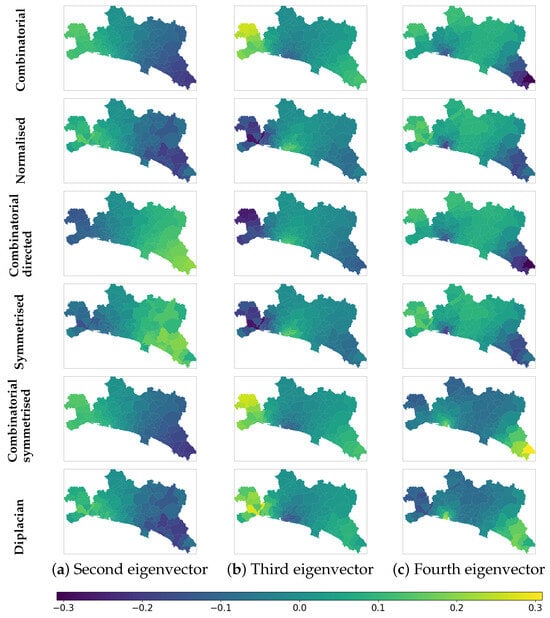
Figure 7.
Eigenvector values of the eigenvalues with the smallest magnitudes associated with different Graph Laplacian matrices on the Region Adjacency graph of Genova Province.
5. Discussion
In light of the outcomes of the experimental tests using different node scoring strategies on Region Adjacency graphs, we now consolidate them to assess their impact on the analysis of mobility networks. The closeness and the betweenness centralities have more meaningful results for the three considered Region Adjacency graphs when using the Earth distance as the edge weights. The degree of centrality could be more significant if there were actual roads following the geodesics between the nodes because it would mean the total distances of constructed highways connected to a sub-region. The Page rank and the eigenvector centralities would be more insightful if additional geographical features were included. Moreover, a negative correlation with the closeness centrality of the undirected graph can be observed. This negative correlation suggests that the decreasing flow velocity on the nodes with higher closeness centrality values can be caused by more information flowing due to the ease these nodes have in accessing the rest of the network. Furthermore, the paths with the highest betweenness centrality values are located in the same area as the sub-regions with lower average node circulation, suggesting that the linking importance of these paths causes some data congestion. The Average Perron node circulation evaluates flows generated by random walks within the network; if a different circulation function is defined, then there might be a different behaviour of the flows due to additional factors. We furthermore consider that the combination of geographical features approaches and Graph Laplacian eigenvectors is an area that can be explored to enhance the study of diffusion processes on a graph.
6. Conclusions and Future Work
In this paper, we presented a variety of node scores that can accomplish the task of identifying relevant node clusters or paths on a particular type of spatial network, i.e., Region Adjacency graphs, which are highly related to the study of mobility flows as many of the flow forecasting models are based on graph topologies. Graph-based structures enable the examination of interactions between different system elements, while also highlighting the most important or vulnerable nodes in the entire network.
Using the Earth distance as the edge weights for the computation of centrality metrics revealed similar patterns for Region Adjacency graphs of different scales. This shows that a sole system of linked nodes on a spatial network can be easily supplied with additional information to obtain further interpretations of the complex system. Implementing the eigendata centrality on the New York State graph using the geographical features of the Deep Gravity model found a hub of relevant nodes correlated with the very same features. Indeed, the cluster of the highest eigendata centrality scores corresponds to the surrounding areas of the sub-regions with the highest normalised data vector values. Moreover, the prototype of the circulation function on the edges defined through the Perron vector of the transition probability matrix was able to complement the flow analysis within the zones of New York State for both the ground truth and the predicted values of the Deep Gravity model.
The combination of mobility prediction models based on geographical features and centrality analysis to assess the topology of a network plays a vital role in facilitating autonomous traffic management decisions, such as suggesting alternative routes for commuters entering a city to ease traffic in specific areas, taking into account mobility predictions and network failure estimates. Graph Theory elements such as edge weights and directionality can provide a model with different interpretation perspectives, particularly in urban, mobility, and geographic networks, where a vast amount of information complements the information obtained from the network topology.
In future work, we intend to monitor mobility data to rebuild traffic flows in urban, regional, and inter-regional contexts by analysing Origin-Destination trajectories, considering diverse, incomplete, and uncertain data, and combining them with meteorological and pollution information. Specifically, the analysis of short-term mobility patterns will enable the classification of user behaviors, such as determining if a route is typically used regularly or occasionally. Furthermore, the development and implementation of new centrality metrics based on the conventional ones that take into account geographical features, such as the eigendata centrality, is desired, as well as the combined centrality and mobility analysis for regions where the flows are available between any pair of zones to bypass the need of defining the minimum flow between neighbouring zones.
Author Contributions
R.A.M.M. and G.P.: Conceptualization; methodology; software; validation; formal analysis; investigation; writing—original draft preparation; writing—review and editing. All authors have read and agreed to the published version of the manuscript.
Funding
This research was partially funded by PON “Ricerca e Innovazione” 2014–2020, Asse IV “Istruzione e ricerca per il recupero”, Azione IV.5 “Dottorati su tematiche Green” DM 1061/2021-FSE REACT-EU.
Data Availability Statement
The boundary data are freely available at [30] (Genova Province) and [31] (United Kingdom). The New York State data and the code used by the Deep Gravity model [9] are available at the repository indicated by the original authors.
Acknowledgments
Our sincere recognition to the anonymous reviewers, whose constructive feedback has enhanced the quality of this manuscript.
Conflicts of Interest
The authors declare no conflicts of interest.
References
- Papadimitriou, F. Geo-Topology: Theory, Models and Applications; Springer: Berlin/Heidelberg, Germany, 2024. [Google Scholar]
- Agryzkov, T.; Tortosa, L.; Vicent, J.F.; Wilson, R. A centrality measure for urban networks based on the eigenvector centrality concept. Environ. Plan. B Urban Anal. City Sci. 2019, 46, 668–689. [Google Scholar] [CrossRef]
- Dees, B.S.; Xu, Y.L.; Constantinides, A.G.; Mandic, D.P. Graph Theory for Metro Traffic Modelling. In Proceedings of the 2021 International Joint Conference on Neural Networks, Shenzhen, China, 18–22 July 2021; pp. 1–5. [Google Scholar]
- Mukherjee, S. Statistical analysis of the road network of India. Pramana 2012, 79, 483–491. [Google Scholar] [CrossRef]
- Zhang, J.; Zheng, Y.; Qi, D. Deep Spatio-Temporal Residual Networks for Citywide Crowd Flows Prediction. In Proceedings of the AAAI Conference on Artificial Intelligence, San Francisco, CA, USA, 4–9 February 2017; Volume 31. [Google Scholar]
- Liang, Y.; Ouyang, K.; Sun, J.; Wang, Y.; Zhang, J.; Zheng, Y.; Rosenblum, D.S.; Zimmermann, R. Fine-Grained Urban Flow Prediction. In Proceedings of the Web Conference 2021, Ljubljana, Slovenia, 19–23 April 2021. [Google Scholar]
- Zhang, Z.; Li, Y.; Song, H.; Dong, H. Multiple dynamic graph based traffic speed prediction method. Neurocomputing 2021, 461, 109–117. [Google Scholar] [CrossRef]
- Zhang, S.; Guo, Y.; Zhao, P.; Zheng, C.; Chen, X. A Graph-Based Temporal Attention Framework for Multi-Sensor Traffic Flow Forecasting. IEEE Trans. Intell. Transp. Syst. 2022, 23, 7743–7758. [Google Scholar] [CrossRef]
- Simini, F.; Barlacchi, G.; Luca, M.; Pappalardo, L. A deep gravity model for mobility flows generation. Nat. Commun. 2021, 12, 6576. [Google Scholar] [CrossRef]
- Oehlers, M.; Fabian, B. Graph Metrics for Network Robustness—A Survey. Mathematics 2021, 9, 895. [Google Scholar] [CrossRef]
- Wan, Z.; Mahajan, Y.; Kang, B.W.; Moore, T.J.; Cho, J.H. A Survey on Centrality Metrics and Their Network Resilience Analysis. IEEE Access 2021, 9, 104773–104819. [Google Scholar] [CrossRef]
- Henry, E.; Bonnetain, L.; Furno, A.; Faouzi, N.E.E.; Zimeo, E. Spatio-Temporal Correlations of Betweenness Centrality and Traffic Metrics. In Proceedings of the 2019 6th International Conference on Models and Technologies for Intelligent Transportation Systems, Cracow, Poland, 5–7 June 2019; pp. 1–10. [Google Scholar]
- Tian, Z.; Jia, L.; Dong, H.; Su, F.; Zhang, Z. Analysis of Urban Road Traffic Network Based on Complex Network. Procedia Eng. 2016, 137, 537–546. [Google Scholar] [CrossRef]
- Ye, J.; Zhao, J.; Ye, K.; Xu, C. How to Build a Graph-Based Deep Learning Architecture in Traffic Domain: A Survey. IEEE Trans. Intell. Transp. Syst. 2022, 23, 3904–3924. [Google Scholar] [CrossRef]
- Pan, S.; Ling, S.; Jia, N.; Liu, Y.; He, Z. On the dynamic vulnerability of an urban rail transit system and the impact of human mobility. J. Transp. Geogr. 2024, 116, 103850. [Google Scholar] [CrossRef]
- Chung, F.R.K. Laplacians and the Cheeger Inequality for Directed Graphs. Ann. Comb. 2005, 9, 1–19. [Google Scholar] [CrossRef]
- Li, Y.; Zhang, Z.L. Digraph Laplacian and the Degree of Asymmetry. Internet Math. 2012, 8, 381–401. [Google Scholar] [CrossRef]
- Veerman, J.J.P.; Lyons, R. A primer on Laplacian dynamics in directed graphs. arXiv 2020, arXiv:2002.02605. [Google Scholar] [CrossRef]
- Brandes, U. A faster algorithm for betweenness centrality. J. Math. Sociol. 2001, 25, 163–177. [Google Scholar] [CrossRef]
- Page, L.; Brin, S.; Motwani, R.; Winograd, T. The PageRank Citation Ranking: Bringing Order to the Web; Technical Report 1999-66; Stanford InfoLab: Stanford, CA, USA, 1999. [Google Scholar]
- Berkhin, P. A Survey on PageRank Computing. Internet Math. 2005, 2, 73–120. [Google Scholar] [CrossRef]
- Bonacich, P. Factoring and weighting approaches to status scores and clique identification. J. Math. Sociol. 1972, 2, 113–120. [Google Scholar] [CrossRef]
- Caughman, J.; Veerman, J. Kernels of Directed Graph Laplacians. Electron. J. Comb. 2006, 13. [Google Scholar] [CrossRef]
- Zhang, S.; Zheng, H.; Su, H.; Yan, B.; Liu, J.; Yang, S. GACAN: Graph Attention-Convolution-Attention Networks for Traffic Forecasting Based on Multi-Granularity Time Series. In Proceedings of the 2021 International Joint Conference on Neural Networks, Shenzhen, China, 18–22 July 2021; pp. 1–8. [Google Scholar]
- Das, K.C. An improved upper bound for Laplacian graph eigenvalues. Linear Algebra Its Appl. 2003, 368, 269–278. [Google Scholar] [CrossRef][Green Version]
- Hasanzadeh, A.; Liu, X.; Duffield, N.G.; Narayanan, K.R.; Chigoy, B.T. A Graph Signal Processing Approach For Real-Time Traffic Prediction In Transportation Networks. arXiv 2017, arXiv:1711.06954. [Google Scholar]
- Barthélemy, M. Spatial networks. Phys. Rep. 2011, 499, 1–101. [Google Scholar] [CrossRef]
- Maria, E.; Budiman, E.; Haviluddin; Taruk, M. Measure distance locating nearest public facilities using Haversine and Euclidean Methods. J. Physics: Conf. Ser. 2020, 1450, 012080. [Google Scholar] [CrossRef]
- Liang, Y.; Zhu, J.; Ye, W.; Gao, S. Region2Vec: Community detection on spatial networks using graph embedding with node attributes and spatial interactions. In Proceedings of the SIGSPATIAL ’22: 30th International Conference on Advances in Geographic Information Systems, New York, NY, USA, 1–4 November 2022. [Google Scholar]
- Comune di Genova. Matrici dei Viaggi Origine-Destinazione. Available online: https://dati.comune.genova.it/dataset/matrici-dei-viaggi-origine-destinazione (accessed on 25 September 2024).
- UK Data Service. Census Boundary Data. Available online: https://ukdataservice.ac.uk/learning-hub/census/other-information/census-boundary-data/ (accessed on 25 September 2024).


Disclaimer/Publisher’s Note: The statements, opinions and data contained in all publications are solely those of the individual author(s) and contributor(s) and not of MDPI and/or the editor(s). MDPI and/or the editor(s) disclaim responsibility for any injury to people or property resulting from any ideas, methods, instructions or products referred to in the content. |
© 2024 by the authors. Licensee MDPI, Basel, Switzerland. This article is an open access article distributed under the terms and conditions of the Creative Commons Attribution (CC BY) license (https://creativecommons.org/licenses/by/4.0/).