The Spatial Impact of PM_2.5 Pollution on Economic Growth from 2012 to 2022: Evidence from Satellite and Provincial-Level Data in Thailand

Abstract

This study examines the spatial relationship of PM_2.5 concentrations across provinces in Thailand and explores the relationship between socio-economic factors and PM_2.5 levels from 2012 to 2022. The study results indicate that PM_2.5 pollution in Thailand is spatially clustered, meaning that PM_2.5 spills over into nearby provinces and is not confined to a single area. The factors that positively affect PM_2.5 concentrations include population density and energy consumption per capita, while industrial density has a negative effect on PM_2.5 levels. Additionally, an Environmental Kuznets Curve (EKC) analysis found that the Gross Provincial Product (GPP) per capita has a U-shaped relationship with the PM_2.5 concentration. In the initial stage of economic growth, as the GPP per capita increases, PM_2.5 concentrations gradually decrease. However, once income reaches USD 56,715 and the economy becomes significantly large, further increases in GPP per capita lead to rising PM_2.5 concentrations. In other words, during the early phase of economic development, PM_2.5 pollution does not intensify significantly. However, once Thailand’s economy reaches a certain scale, continued economic expansion exacerbates PM_2.5 pollution, leading to greater economic and social consequences. The study highlights the importance of integrated collaboration among various organizations in mitigating the widespread impacts of PM_2.5 pollution.

1. Introduction

Air pollution is a global issue, particularly in low- and middle-income countries, which serve as industrial production hubs and often rely on low technology. Additionally, heavy vehicle usage and traffic congestion contribute significantly to air pollution [1]. Air pollution has severe health consequences and can lead to stroke, heart disease, lung cancer, and respiratory diseases. In 2019, approximately 99% of the world’s population lived in areas where the air quality was poor and did not meet the good air quality standards set by the World Health Organization (WHO). The WHO estimated that air pollution caused approximately 4.2 million premature deaths in 2019, with 89% of these deaths occurring in low- and middle-income countries. Most of the affected populations were in Southeast Asia and the Western Pacific regions [2].

Thailand experienced economic growth of approximately 24.62% from 2012 to 2022, as measured by GDP (Gross Domestic Product) [3], caused by the expansion of its urbanization and industrial sectors. Both factors cause air pollution problems, especially in terms of Particulate matter 2.5 (PM_2.5) and Sulfur dioxide (SO₂) emissions from vehicles and fuel, residential, and industrial uses [4]. PM_2.5 and SO₂ are considered major causes of air pollution that greatly affect the economy, the environment, and public health. SO₂ is a component of particulate matter (PM) and has become a major problem in Thailand, particularly in areas with high economic activity, industry, and urbanization. This pollution contributes to environmental degradation and indirectly impacts Thailand’s economy. It has also been found that air pollution has resulted in economic costs as high as 210,603 million baht in 1990 and 871,300 million baht in 2013, when adjusted to 2018 currency values [1].

This is a critical issue in Thailand as it imposes significant economic, public health, and environmental costs. In particular, PM_2.5 and SO₂, which originate from both domestic and neighboring countries’ economic activities, contribute to severe pollution levels. This study focuses on the socio-economic factors influencing PM_2.5 concentrations across provinces. By analyzing how each socio-economic factor affects PM_2.5 levels, the findings can help formulate policy recommendations for economic planning aimed at addressing air pollution and promoting environmentally friendly and sustainable growth. These efforts align with Thailand’s 20-Year National Strategy (2018–2037), the Master Plan of the National Strategy (2018–2037), and the National Reform Plan on Natural Resources and Environment, all of which emphasize the development of an eco-friendly economy and long-term sustainable growth. The goal is to control air pollution levels, ensuring that they do not exceed the international standards set by Thailand [5].

However, a research gap remains, as previous studies have predominantly relied on provincial-level, ground-based data in Thailand [6,7,8,9]. To cover this research gap, the main objective of this study is to utilize satellite data from the Modern-Era Retrospective Analysis for Research and Applications, Version 2 (MERRA-2) to analyze the spatial correlations of PM_2.5 within the model and examine the relationship between air pollution and socio-economic factors in Thailand using the EKC framework and a spatial econometric model. This methodological approach differs from previous studies. The study results confirm that provinces with high economic activity and energy consumption intensity and sizable populations tend to experience severe PM_2.5 pollution. Additionally, PM_2.5 is a nationwide issue that affects all provinces rather than being confined to a single region. Therefore, the government should implement integrated policies at the national level rather than addressing the problem in isolation within individual provinces. Based on the case study of Thailand, this study’s methods and policy recommendations can be applied to other developing Asian countries facing similar air pollution challenges.

In Section 2, we introduce the background used for selecting Thailand as the scope area of this research. In Section 3, we discuss the theoretical framework of this study. Section 4 describes the analytical methods used in the study, and Section 5 displays the empirical results and provides discussions based on the results. Finally, we provide a conclusion and policy implications in Section 7.

2. Study Background

2.1. The Economic Characteristics of Thai Provinces

Table 1. All provinces of Thailand.

Regions	Provinces
NORTHEASTERN (NE)	KHON KAEN, UDON THANI, LOEI, NONG KHAI, MUKDAHAN, NAKHON PHANOM, SAKON NAKHON, KALASIN, NAKHON RATCHASIMA, CHAIYAPHUM, YASOTHON, UBON RATCHATHANI, ROI ET, BURI RAM, SURIN, MAHA SARAKHAM, SI SA KET, NONGBUA LAMPHU, AMNAT CHAREON, BUENG KAN
NORTHERN (NO)	CHIANG MAI, LAMPANG, UTTARADIT, MAE HONG SON, CHIANG RAI, PHRAE, LAMPHUN, NAN, PHAYAO, NAKHON SAWAN, PHITSANULOK, KAM PHAENG PHET, UTHAI THANI, SUKHOTHAI, TAK, PHICHIT, PHETCHABUN
SOUTHERN (SO)	PHUKET, SURAT THANI, RANONG, PHANGNGA, KRABI, CHUMPHON, NAKHON SI THAMMARAT, SONGKHLA, SATUN, YALA, TRANG, NARATHIWAT, PHATTHALUNG, PATTANI
EASTERN (EA)	CHON BURI, CHACHOENGSAO, RAYONG, TRAT, CHANTHABURI, NAKHON NAYOK, PRACHIN BURI, SA KAEW
WESTERN (WE)	RATCHABURI, KANCHANABURI, PHACHUAP KHIRI KHAN, PHETCHABURI, SUPHAN BURI, SAMUT SONGKHRAM
CENTRAL (CE)	SARABURI, SINGBURI, CHAI NAT, ANG THONG, LOP BURI, PHRA NAKHON SRI AYUTHAYA
BANGKOK AND VICINITIES (BKK&VIC)	BANGKOK METROPOLIS, SAMUT PRAKAN, PATHUM THANI, SAMUT SAKHON, NAKHON PATHOM, NONTHABURI

presents the geographical regions of Thailand and the provinces located within each region. According to Table 1, the economic structure of the NE region is as follows: the agricultural sector accounts for 19.6%, the industrial sector for 20.2%, and the service sector for 53.1%. The labor structure of the NE region is as follows: the agricultural sector comprises 53.1% of the workforce, the industrial sector 8.0%, and the service sector 39.0%. The majority of the labor force is employed in the agricultural sector, as well as in trading and general employment [10].

In the case of the NO region, the agricultural sector accounts for 24.5% of the region’s economy, the industrial sector for 19.6%, and the service sector for 55.9%. In terms of its labor structure, the agricultural sector comprises 43.8% of the workforce, the industrial sector 10.2%, and the service sector 45.9%. It is evident that the majority of the labor force is employed in the agricultural sector and works as traders or general laborers, similar to in the NE region [10].

In the SO region, the agricultural sector accounts for 26.2% of the region’s economy, the industrial sector for 16.4%, and the service sector for 57.4%. The labor structure in the SO region is as follows: the agricultural sector comprises 41.9% of the workforce, the industrial sector 8.7%, and the service sector 49.4%. The majority of the labor force is employed in the agricultural sector, primarily working in rubber plantations, and in the tourism industry, providing services [10].

The economic structure of the EA region is as follows: the agricultural sector accounts for 7.2%, the industrial sector for 62.6%, and the service sector for 30.2%. The labor structure of the EA region is as follows: the agricultural sector comprises 22.1% of the workforce, the industrial sector 27.2%, and the service sector 50.7%. The majority of the labor force is employed in the service and industrial sectors, as this area is an industrial estate with a large number of workers residing there [10].

As for the WE region, the agricultural sector accounts for 21.3%, the industrial sector for 29.7%, and the service sector for 48.9%. In terms of its labor distribution, 32.6% of the workforce is employed in agriculture, 15.3% in industry, and 52.1% in services. This region primarily focuses on tourism and agriculture [10].

Regarding the economic structure of the CE region, the agricultural sector accounts for 6.5%, the industrial sector 58.0%, and the service sector 35.5%. In this region, 21.1% of the workforce is employed in agriculture, 28.8% in industry, and 50.1% in services. This region is home to large industrial estates, with most of the labor force working in the service and industrial sectors [10].

Finally, in the BKK&VIC region, the agricultural sector accounts for 0.6%, the industrial sector for 22.4%, and the service sector for 77.0%. In this region, 2.7% of the workforce is employed in agriculture, 27.4% in industry, and 69.9% in services. Bangkok and its vicinity are major economic hubs featuring industrial estates, business districts, department stores, and residential areas. Notably, the economic output of Bangkok and its vicinity accounts for nearly half of the country’s GDP (47.6% of Thailand’s GDP in 2022) [10].

Table 2. Gross Regional Product (GRP), GRP per capita, and GDP contributions of the seven regions (USD).

Regions	2022 GRP	2022 GRP per Capita	2022 GRP per Capita (PPP)	GDP Contribution in 2022
NORTHEASTERN (NE)	USD 498 billion	USD 2724	USD 9009	10.2%
NORTHERN (NO)	USD 373 billion	USD 3329	USD 11,012	7.9%
SOUTHERN (SO)	USD 394 billion	USD 4053	USD 13,407	8.2%
EASTERN (EA)	USD 931 billion	USD 14,639	USD 48,421	17.2%
WESTERN (WE)	USD 180 billion	USD 4934	USD 16,321	3.6%
CENTRAL (CE)	USD 255 billion	USD 8074	USD 26,705	5.4%
BANGKOK AND VICINITIES (BKK&VIC)	USD 2.2 trillion	USD 13,210	USD 43,693	47.6%

Note: The source for PPP is from World Bank [11] and other data are from NESDC [12].

illustrates the gross regional product (GRP), GRP per capita, and GDP contributions of the seven geographical regions. As seen in Table 2, the region with the highest GRP is the BKK&VIC region, followed by the EA region in second place, NE region in third, and SO region in fourth. The remaining regions—NO, CE, and WE—have the lowest economic activity in Thailand. However, if we examine the GRP per capita of the CE region, we find that it ranks third highest in the country, as this region is also an industrial manufacturing hub [10].

Figure 1 shows the PM_2.5 concentration in each province of Thailand from 2012 to 2022. It can be seen that the PM_2.5 concentration follows a similar pattern throughout this period. The highest concentrations are clustered in the central part of the map, which includes the BKK&VIC and CE regions, the upper part of the map, representing the NO region, and the right side of the map, corresponding to the NE region. These areas consistently experience severe PM_2.5 pollution problems.

2.2. Relevance of Satellite Data and the Industrial Census Survey in Thailand

Several studies have examined the relationship between socio-economic factors and satellite data indicators in Thailand. Puttanapong et al. [13] suggested the novel integration of satellite data and spatial analytical methods. Sangkasem and Puttanapong [14] explored the use of nighttime light (NTL) data from the Defense Meteorological Satellite Program-Operational Linescan System (DMSP-OLS) as an economic indicator. Prasertsoong and Puttanapong [15] aimed to predict economic growth and urban land-use change in one of the fastest-growing areas in Thailand—the Ban Chang District—from 2021 to 2030.

This study is inspired by the work of [16,17,18]. Building on their approach, this research advances the concept by utilizing air pollution data from the MERRA-2 satellite, which provides provincial-level data for Thailand. Spatial analysis and spatial econometrics are applied to investigate the spatial spillover effects of PM_2.5 pollution. The use of MERRA-2 satellite data helps address gaps caused by incomplete air pollution records in Thailand. Additionally, this study identifies an inflection point that reflects the turning point of the relationship between PM_2.5 pollution and economic growth. These findings could support the development of environmental policies in Thailand, particularly in addressing PM_2.5 pollution issues. Furthermore, this research contributes to the academic understanding of environmental issues by utilizing publicly available satellite data, which offers a low-cost alternative for pollution studies. The use of this dataset has significant potential for air pollution research in both developed and developing countries, providing a novel approach to studying air pollution problems in the future.

Studies on the accuracy of nighttime light (NTL) data from the Defense Meteorological Satellite Program (DMSP) and the Visible Infrared Imaging Radiometer Suite (VIIRS) found that using DMSP nighttime light data for spatial inequality analyses in the United States and China led to biased estimations and inconsistent trends [19,20]. Moreover, the accuracy of the DMSP was found to be lower than that of the VIIRS. A literature review also indicated that air pollution data obtained from MERRA-2 tends to underestimate pollution levels by about 30% because of the coarse resolution of its spatial satellite images. Many studies recommend combining satellite data with ground-based data to enhance the accuracy and reliability of air pollution measurements [21,22,23]. It is known that although MERRA-2 data cannot provide 100% accuracy in measuring air pollution levels, it can effectively reflect air pollution concentration patterns in different areas with an accuracy comparable to ground-based data [24,25].

Therefore, it is recommended that MERRA-2 data be used to fill gaps in incomplete datasets in various areas, improving data coverage. This approach is particularly useful for tracking air pollution in regions where ground-based data are unavailable.

3. Theoretical Framework

3.1. Environmental Kuznets Curve

The Environmental Kuznets Curve (EKC) theory is frequently used to describe the connection between economic growth and environmental quality. It proposes that this relationship is non-linear and can differ across countries. Although empirical studies confirm the EKC hypothesis in certain cases, it is not universally applicable to all types of environmental degradation, income groups, or national circumstances. This study identifies five distinct EKC patterns [26]:

(1) A monotonic relationship. (2) A decreasing monotonic relationship. (3) An inverted U-shaped pattern. (4) A U-shaped pattern which contradicts the typical EKC pattern. (5) A flat pattern, which suggests that income levels have no significant impact on emissions.

3.2. Stochastic Impacts by Regression on Population, Affluence, and Technology Model (STIRPAT Model)

The STIRPAT model extends the IPAT and ImPACT frameworks, which are limited to capturing the non-monotonic or non-proportional effects of influencing factors. In contrast, the STIRPAT model has been effectively used to examine how various driving forces contribute to different environmental impacts [27]:

$$I_i=a{P}_i^b{A}_i^c{T}_i^d{e}_i$$

(1)

The model retains the multiplicative structure of the equation I = PAT, where environmental impact (I) is determined by population (P), affluence (A), and technology (T).

After taking logarithms, the model takes the following form:

$${lnI}_{it}=a+b\left({lnP}_{it}\right)+c\left({lnA}_{it}\right)+d\left({lnT}_{it}\right)+e_i$$

(2)

In this study, P is the population density, A is the gross regional and provincial product per capita (GPP) and industrial density, and T is the energy consumption per capita. The energy consumption per capita is used as technology (T) proximity in the STIRPAT model that follows [18].

Table 3. A review of the relationship between economic growth and pollution.

EKC Patterns	Authors	Dependent Variables	Independent Variables
Monotonic rising curve	[28,29,30,31,32,33]	Annual emissions of CO2	Gross Regional Product (GRP) per capita and square, Energy Consumption, Output, Foreign Direct Investment (FDI), Transport energy consumption, Labor Force, Exports and Imports
Inverted U shape	[34,35]	Annual emissions of NO2, SO2, suspended particulate matter	GRP per capita and square, Population density, Industry shares in GRP, Trade intensity
U shape	[32,36,37,38,39,40]	Annual emissions of CO2, SO2, suspended particulate matter	GRP per capita, Population growth, Spatial intensity of economic activity, Energy consumption, FDI, Transport energy consumption

presents three EKC patterns: the monotonic rising curve, the inverted U shape, and the U shape. It also includes studies on various EKC patterns related to air pollution issues and the independent variables that influence the dependent variable. In this study, the independent variables from the table are used as reference variables. Additionally, we reviewed further research to confirm the relationship between the dependent and independent variables in the context of air pollution issues.

3.3. Socio-Economic Impact of PM_2.5

Zhu et al. [41] discovered that in urban agglomerations along China’s Yangtze River, rising PM_2.5 levels were driven by factors like population growth, urbanization, and higher per capita GDP. They also found that a larger share of the population being non-agricultural was associated with increased PM_2.5, while foreign direct investment (FDI) was linked to lower PM_2.5 levels—possibly due to the adoption of cleaner technologies or the enforcement of stricter environmental policies. Chen et al. [42] investigated how income levels relate to PM_2.5 emissions and found that higher income levels are associated with lower PM_2.5 concentrations. This implies that PM_2.5 pollution tends to be more severe in lower-income countries than in wealthier ones. One study found that industrial emissions significantly impact PM_2.5 concentrations [43]. It also identified population density as an important factor contributing to PM_2.5 levels. Similarly, Yang et al. [44] identified industrial output and climate as the two most influential factors affecting PM_2.5 emissions. They also found that construction activity, road density, and fossil fuel use significantly contribute to PM_2.5 levels, along with environmental conditions such as the state of the ecological environment. At the national level, its findings revealed the following relationships: Zhang et al. [45] reported that PM_2.5 emissions were negatively associated with the urban population ratio (URB), per capita GDP (GDP), and energy intensity (ENI). In contrast, PM_2.5 emissions showed a positive association with the share of the secondary industry in the GDP (SEC), the length of highways (WAY), the total volume of urban central heating (HEA), and the extent of built-up areas (BUI). References [46,47] identified several key factors influencing the Air Quality Index (AQI) in Jinan City and Hohhot, including energy consumption, emissions of SO₂, NOx, particulate matter, PM_2.5, and PM10. They also found that meteorological conditions—such as average wind speed and atmospheric pressure—and emissions of sulfur dioxide, nitrogen oxides, and particulates significantly affect air quality, contributing positively to changes in the AQI.

Based on our literature reviews and Table 3, we can state that population density, GPP per capita, industrial density, energy intensity, and other variables affect PM_2.5 pollution both directly and indirectly. Most air pollution studies in our literature review focus on the Environmental Kuznets Curve (EKC) pattern in developing countries with economic structures similar to that of Thailand. Therefore, the researchers use the above case studies as benchmarks against which to compare the results of this Thailand case study. Hence, this study sets hypotheses based on these literature reviews.

4. The Analytical Methods

In this study, Equation (2) serves as the base model for setting up and analyzing both non-spatial and spatial econometric models to examine the relationship between air pollution and economic factors. Specifically, the models consider P to be the population density, A to be the gross regional and provincial product per capita (GPP) and industrial density, and T to be the energy consumption per capita.

The data for this study were obtained from various sources, as shown in

Table 4. Description of the data.

Type	Variables	Description	Years	Sources	Expected Sign
Dependent Variable	PM2.5	The PM2.5 concentration in each province (${\mathsf{\mu }\mathrm{g}/\mathrm{m}}^3$)	2012 2017 2022	Modern-Era Retrospective analysis for Research and Applications, Version 2 (MERRA-2) bands DUSMASS25 + OCSMASS+ BCSMASS + SSSMASS25 + SO4SMASS × (132.14/96.06)
Independent Variables	Population density (Pop_dens)	A variable that represents the province’s population density relative to its size. (Unit/km2)	2012 2017 2022	Office of the National Economic and Social Development Council (NESDC)	+
	Gross Provincial Product per capita (GPPpc)	A variable that represents the economic growth per capita in each province, which is how much economic growth per capita is in that province (Baht/person)	2012 2017 2022	Office of the National Economic and Social Development Council (NESDC)	+/−
	Industrial density (Indus_dens)	A variable that shows the density of industry in each province, which shows that if that province has a high industrial density, more air pollution is released, especially PM2.5 (Baht/km2)	2012 2017 2022	Thailand Industrial Census Survey	+/−
	Energy consumption per capita (Energy_cons_pc)	A variable that shows the province’s economic activities, using energy consumption per capita as an indicator (kWh/person)	2012 2017 2022	Metropolitan Electricity Authority (MEA) and Provincial Electricity Authority (PEA)	+

, including satellite data (MERRA-2), the Industrial Census Survey of Thailand (NSO), and the Gross Regional and Provincial Product (NESDC). The dataset covers the years 2012, 2017, and 2022 and consists of the panel data for each province in each of those years in Thailand.

As previously noted, a bivariate Moran scatter plot builds on the traditional Moran scatter plot by extending it to two variables. While the original plot compares a variable with its own spatial lag, the bivariate version compares one variable on the x-axis with the spatial lag of a different variable on the y-axis. Essentially, this approach measures how the value of one variable in a specific location is spatially correlated with the values of another variable in neighboring areas [48].

$$I_i^B={cx}_i{\sum }_j{w}_{ij}{y}_i$$

(3)

where $c$ is a constant and $w_{ij}$ are the elements of the spatial weight matrix. As with its global counterpart, this statistic needs to be interpreted with caution since it ignores the in situ correlation between the two variables ($x_i$ and $y_i$).

Econometric Models

The Pesaran’s CD Test and Breusch and Pagan LM Test exhibited cross-sectional dependence (see

Table A1. Pesaran’s CD Test and Breusch and Pagan LM Test.

Variables	Pesaran’s CD Test	Breusch and Pagan LM Test
LnPM2.5	91.015 ***	57.82 ***
LnGPPpc	59.917 ***
LnGPPpc2	59.903 ***
LnIndus_dens	45.223 ***
LnEnergy_cons_pc	46.218 ***
LnPop_dens	2.151 **

Note: ** p < 0.05, *** p < 0.01.

in Appendix A), indicating that the random effects model is more appropriate than the pooled-OLS model. The random effects model allows for the inclusion of time-invariant variables (e.g., geographic location), which are critical for spatial modeling and not considered in the fixed effects model. In this study, a non-spatial and three spatial random effects models are used: the Spatial Lag Random Effects Model (SLM), the Spatial Error Random Effects Model (SEM), and the Spatial Durbin Random Effects Model (SDM).

The non-spatial random effects model is used to provide a benchmark for the other models and is expressed as follows:

$$\begin{array}{l}{Ln{PM}_{2.5}}_{it}=a+{\beta }_1{LnPoP\_dens}_{it}+{\beta }_2{LnGPPpc}_{it}+{\beta }_3{{LnGPPpc}^2}_{it}\\ +{\beta }_4{LnIndus\_dens}_{it}+{\beta }_5{LnEnergy\_cons\_pc}_{it}+{\mu }_i+{\mathsf{\lambda }}_i+{\epsilon }_{it}\end{array}$$

(4)

Here, $i$ denotes the province; $t$ denotes the time periods (2012, 2017, and 2022); ${\mu }_i$ is the spatial fixed effects, indicating the city-specific and time-invariant variables that are not included in the model. ${\mathsf{\lambda }}_i$ is the time-fixed effects, indicating time-specific and city-invariant variables that are not included in the model and must be controlled for; and ${\epsilon }_{it}$ is the random error.

The first spatial random effects model applied in this study is the SLM, which captures the spatial effects of neighboring regions, known as the spatial spillover effect. This model is denoted in Equation (5).

$$\begin{array}{l}{Ln{PM}_{2.5}}_{it}=a+\rho W{Ln{PM}_{2.5}}_{it}+{\beta }_1{LnPop\_dens}_{it}+{\beta }_2{LnGPPpc}_{it}+{\beta }_3{{LnGPPpc}^2}_{it}\\ +{\beta }_4{LnIndus\_dens}_{it}+{\beta }_5{LnEnergy\_cons\_pc}_{it}+{\mu }_i+{\mathsf{\lambda }}_i+{\epsilon }_{it}\end{array}$$

(5)

In this equation, $\rho$ is the spatial autoregressive coefficient, indicating the spatial spillover effect of PM_2.5, and $WLn{PM}_{2.5it}$ is the spatially lagged dependent variable of PM_2.5.

The second spatial random effects model is the SEM, which introduces spatial dependence in the error term and captures unobserved spatially correlated factors among regions. This model is written as follows:

$$\begin{gathered} {Ln{PM}_{2.5}}_{it}=a+{\beta }_1{LnPop\_dens}_{it}+{\beta }_2{LnGPPpc}_{it}+{\beta }_3{{LnGPPpc}^2}_{it}+ \\ {\beta }_4{LnIndus\_dens}_{it}+{\beta }_5{LnEnergy\_cons\_pc}_{it}+{\mu }_i+{\mathsf{\lambda }}_i+{\epsilon }_{it}, \end{gathered}$$

(6)

where ${\epsilon }_{it}=\gamma W{\epsilon }_{it}+{\mathrm{\varnothing }}_{it}$.

$\gamma$ denotes the unknown coefficient of the spatial autocorrelation error term, ${W\epsilon }_{it}$ is the spatial autocorrelated error term, and ${\varnothing }_{it}$ is the error term.

The final spatial random effects model is the SDM. The SDM is an extended version of the SLM that considers not only the spatial impact of the dependent variable but also the spatial spillover effect of the independent variable. It can be expressed as follows:

$$\begin{array}{l}{Ln{PM}_{2.5}}_{it}=a+{\beta }_1{LnPop\_dens}_{it}+{\beta }_2{LnGPPpc}_{it}+{\beta }_3{{LnGPPpc}^2}_{it}+\\ {\beta }_4{LnIndus\_dens}_{it}+{\beta }_5{LnEnergy\_cons\_pc}_{it}+W_1{Ln{PM}_{2.5}}_{it}+W_2{LnPop\_dens}_{it}+\\ W_3{LnGPPpc}_{it}+W_4{{LnGPPpc}^2}_{it}+W_5{LnIndus\_dens}_{it}+W_6{LnEnergy\_cons\_pc}_{it}\\ +{\mu }_i+{\mathsf{\lambda }}_i+{\epsilon }_{it}\end{array}$$

(7)

Here, $W_1$ through $W_6$ are the weight coefficients of the explanatory variables.

5. Empirical Results and Discussion

As seen in

Table 5. Empirical results (spatio-temporal characteristics of PM_2.5 pollution) of Moran’s I statistical test.

Variables	Year	Moran’s I	E(I)	SE(I)	Z(I)	p-Value
PM2.5	2012	0.945	−0.013	0.092	10.435	0.000
	2017	0.928	−0.013	0.090	10.460	0.000
	2022	0.935	−0.013	0.090	10.499	0.000

, the researchers used the K-nearest neighbors (K-NN) method to construct the spatial weight matrix because K-NN can generate a weight matrix regardless of the absolute distance. Phuket, being an island, does not share a border with any other province in Thailand. The Moran’s I statistical test for PM_2.5 data across the three years (2012, 2017, and 2022) found Moran’s I values of 0.945, 0.928, and 0.935, respectively. These values are close to 1 and are statistically significant at the 1% level (p-value < 0.001). This indicates that PM_2.5 concentrations in each province exhibit a spatial clustering pattern. In other words, the PM_2.5 concentration in one province influences the PM_2.5 concentration in nearby provinces, forming a clustered distribution. Therefore, this study employs spatial econometric methods, including the Spatial Lag Model (SLM), Spatial Error Model (SEM), and Spatial Durbin Model (SDM), to analyze the spread and spatial effects of PM_2.5 pollution across provinces.

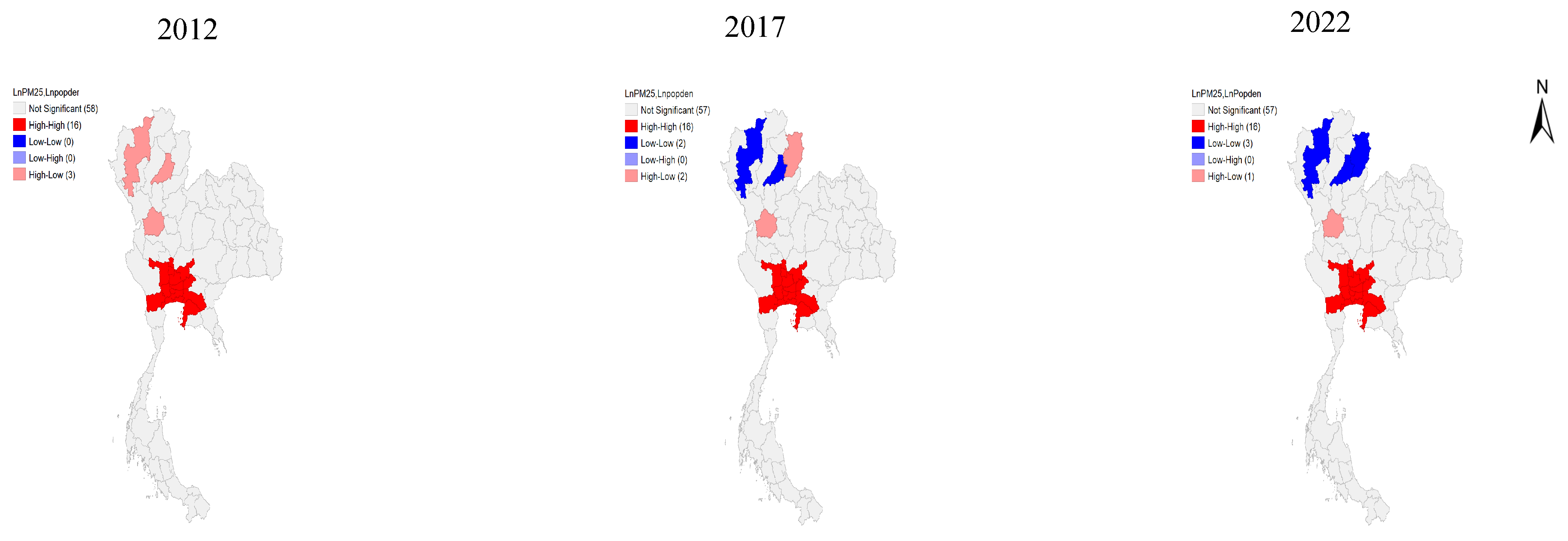
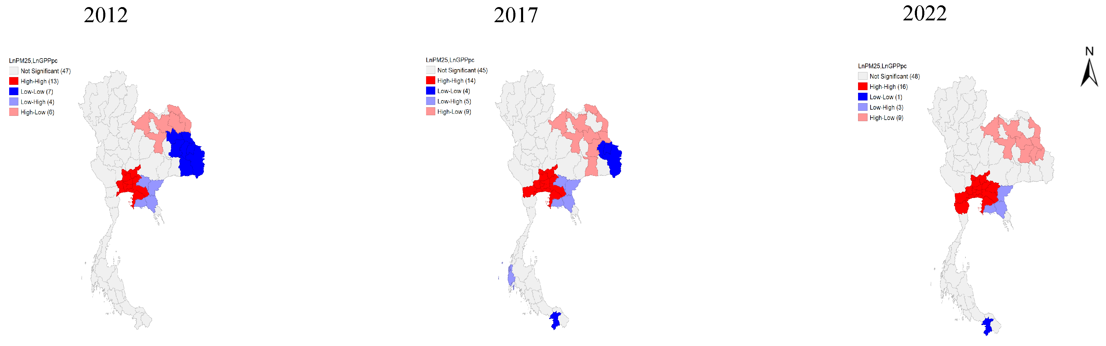
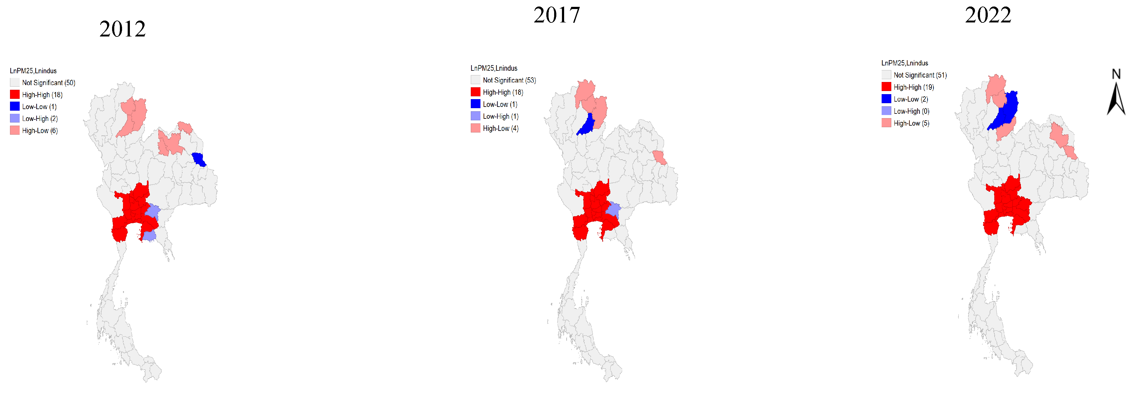
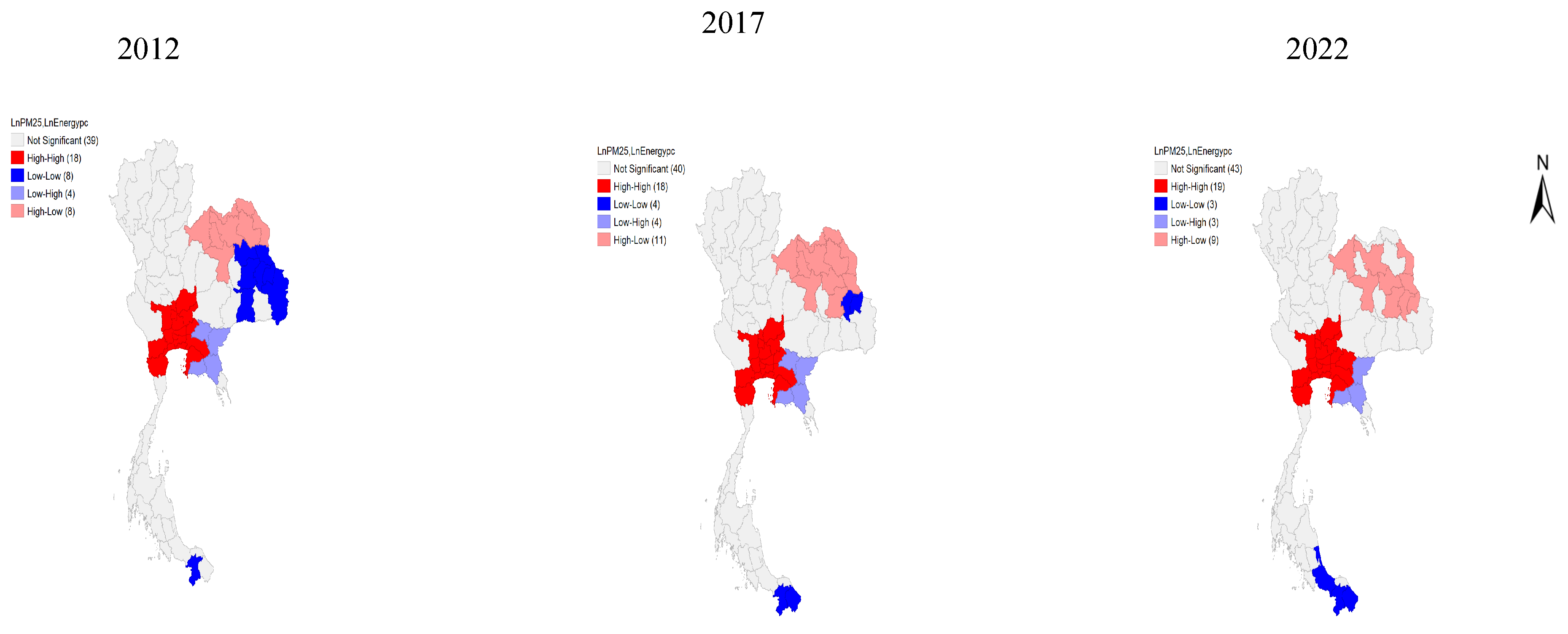
5.1. Bivariate Local Moran’s I Results

Figure 2 illustrates the relationship between PM_2.5 concentration and population density from 2012 to 2022. The dark red areas on the map indicate regions with a high PM_2.5 concentration and high population density (High–High clusters), which are primarily clustered in central Thailand, particularly in the BKK&VIC and CE regions.

In contrast, the dark blue areas on the upper side of the map represent the NO region of Thailand, which is predominantly mountainous and forested. Most residents in this region are farmers engaged in sugarcane and corn cultivation for animal feed, and forest burning is commonly practiced to collect forest products. These areas have a low population density compared to the BKK&VIC region, where business districts offer diverse job opportunities. As a result, many workers from rural areas migrate permanently to the BKK&VIC region in search of employment. This migration trend explains why NO has a lower population density [10,49,50].

Figure 3 illustrates the relationship between the PM_2.5 concentration and GPP per capita from 2012 to 2022. The dark red areas on the map represent those with a high PM_2.5 concentration and high GPP per capita (High–High clusters), which are primarily found in central Thailand, particularly in the BKK&VIC and CE regions. These regions are Thailand’s major economic and industrial hubs, characterized by high economic activity, shopping malls, residential areas, and business districts [10,50,51].

In contrast, the light blue areas at the bottom right of the map represent areas with a low PM_2.5 concentration but high GPP per capita (Low–High clusters). These regions (EA) include industrial estates, special economic zones, and the Eastern Economic Corridor (EEC), which are close to the Gulf of Thailand. The sea breeze helps disperse pollutants, resulting in lower PM_2.5 concentrations despite high economic activity [10,51,52].

On the right-hand side of the map, the pink areas in the NE region of Thailand contains areas with a high PM_2.5 concentration but low GPP per capita (High–Low clusters). The dark blue areas indicate regions with low PM_2.5 concentration and low Energy consumption per capita (Low-Low clusters). These areas are predominantly agricultural, and most residents are farmers engaged in rice cultivation and gardening. Due to the low market value of agricultural products, these provinces have a low GPP per capita. Additionally, the open burning of agricultural waste is a common practice in these areas, as farmers clear fields quickly for the next planting season [10,50,53].

Figure 4 illustrates the relationship between PM_2.5 concentration and industrial density from 2012 to 2022. The dark red areas, the BKK&VIC and CE regions (High–High clusters), and the light blue areas, the EA region (a Low–High cluster), on the map are interpreted similarly to those in previous figures.

Found on the upper half of the map, the NO region of Thailand is characterized by mountainous and forested landscapes. Most residents in this area are farmers engaged in sugarcane and corn cultivation for animal feed. Additionally, forest burning is commonly practiced for agricultural purposes and to collect forest products. As a result, this region experiences high PM_2.5 concentrations. These areas are classified as having a high PM_2.5 concentration but low industrial density (High–Low clusters) (pink areas) [10,49,50].

Figure 5 illustrates the relationship between PM_2.5 concentration and energy consumption per capita from 2012 to 2022. For the dark red areas, the BKK&VIC and CE (High–High clusters) regions, and the light blue areas, the EA region (a Low–High cluster), on the map, the interpretation is similar to that in previous figures. The energy consumption in these areas is closely related to their economic activity.

On the right-hand side of the map, the NE region of Thailand shows areas with a high PM_2.5 concentration but low energy consumption per capita (High–Low clusters) (pink areas). The dark blue areas indicate regions with a low PM_2.5 concentration and low energy consumption per capita (Low–Low clusters). The energy consumption per capita is lower in these regions due to lower daily energy usage, as many residents live in rural areas with fewer electronic appliances and lower per capita incomes compared to the BKK&VIC region [10,50,53].

Table 6. Descriptive statistics.

	Obs	2012			2017				2022
		Mean		Min/Max	Mean		Min/Max	Mean		Min/Max
PM2.5	231	19.357 (3.771)	Min Max	11.948 27.001	15.615 (2.083)	Min Max	11.435 19.352	15.704 (2.085)	Min Max	11.323 19.187
Population density	231	279.789 (686.090)	Min Max	16.174 5382.581	300.575 (741.628)	Min Max	18.320 5629.551	312.403 (775.694)	Min Max	19.027 5776.465
GPP per capita	231	139,936.948 (135,805.876)	Min Max	41,474.000 970,023.000	162,737.849 (152,620.342)	Min Max	55,861.466 1,017,235.244	175,189.788 (152,306.472)	Min Max	60,876.433 1,003,496.913
Industrial density	231	50,637,499.189 (159,485,243.578)	Min Max	13,988.457 1,065,949,279.061	72,587,788.251 (228,435,012.632)	Min Max	14,381.052 1,565,100,976.437	82,125,296.321 (230,089,098.661)	Min Max	10,525.159 1,426,639,278.506
Energy consumption per capita	231	1971.658 (1969.084)	Min Max	475.806 10,377.009	2142.582 (1986.598)	Min Max	534.198 11,335.862	2250.422 (1869.915)	Min Max	617.313 10,141.995

Note: standard deviation in parentheses.

presents the characteristics of both the dependent and independent variables used in this study. It displays the mean value of each indicator for all 77 provinces in Thailand in 2012, 2017, and 2022. The units used for each indicator are presented in Table 4.

5.2. Regression Results

Random effects are used as a benchmark for measuring the accuracy of the spatial econometric models (SLM, SEM, and SDM). When comparing these three models, it is evident that they all produce coefficients with the same directional signs. However, if the focus is solely on direct effects, the SEM can be examined, as its statistically significant variables show minimal differences with those of the SLM. On the other hand, if the indirect effect is of interest, the SDM is the most appropriate choice. This is supported by the model fit indicators, including the AIC, BIC, and likelihood ratio test, where the SDM exhibits the lowest AIC and BIC values and the highest likelihood ratio test value.

Table 7. Results of non-spatial, Spatial Lag (SLM), and Error (SEM) Models (Panel Random Effects Regression).

Dependent Variable: LnPM2.5	Random Effects			SLM			SEM
Variables	M1	M2	M3	M4	M5	M6	M7	M8	M9
LnPop_dens	0.130 *** (4.12)	0.133 *** (4.17)	0.102 *** (3.25)	0.150 *** (4.96)	0.151 *** (4.97)	0.122 *** (4.30)	0.055 *** (2.88)	0.055 *** (2.88)	0.050 *** (2.71)
LnGPPpc	−0.256 *** (−3.90)		−3.088 *** (−4.26)	−0.165 *** (−2.67)		−2.860 *** (−4.42)	−0.082 ** (−2.11)		−1.260 *** (−2.95)
LnGPPpc2		−0.100 *** (−3.53)	0.116 *** (3.93)		−0.006 ** (−2.29)	0.111 *** (4.19)		−0.003 * (−1.86)	0.048 *** (2.77)
LnIndus_dens	−0.037 * (−1.93)	−0.380 ** (−2.02)	−0.030 (−1.51)	−0.054 *** (−3.13)	−0.054 *** (−3.13)	−0.460 *** (−2.73)	−0.010 (−0.89)	−0.010 (−0.94)	−0.007 (−0.73)
LnEnergy_cons_pc	0.162 ** (2.49)	0.141 ** (2.19)	0.208 *** (3.25)	0.128 ** (2.16)	0.110 * (1.87)	0.174 *** (3.03)	0.053 (1.40)	0.045 (1.29)	0.063 * (1.69)
Constant	4.541 *** (10.45)	4.541 *** (10.45)	21.370 *** (4.96)	3.630 *** (8.29)	2.643 *** (12.71)	19.628 *** (5.09)	3.171 *** (11.79)	2.685 *** (18.27)	10.224 *** (4.00)
Rho ($\rho )$				0.123 *** (5.21)	0.124 *** (5.25)	0.117 *** (5.64)
Lambda (λ)							0.970 *** (62.21)	0.970 *** (62.50)	0.966 *** (61.78)
Observations	231	231	231	231	231	231	231	231	231
Within R-squared	0.301	0.303	0.290
Between R-squared	0.045	0.038	0.084
Overall R-squared	0.068	0.060	0.118
Log-likelihood				113.675	112.734	122.106	228.474	227.982	232.194
AIC				−211.350	−209.470	−226.211	−440.950	−439.963	−446.390
BIC				−193.810	−181.930	−195.230	−413.409	−412.424	−415.405

Note: z-statistics are reported in parentheses. * p < 0.10, ** p < 0.05, *** p < 0.01.

summarizes the results of the random effects, spatial lag (SLM), and spatial error models (SEM). In the table, the non-spatial regression results are divided into three models: M1, M2, and M3. M1 and M2 are estimated separately by including LnGPPp and LnGPPpc² separately to avoid multicollinearity issues. Although these estimations are divided into two models, their results remain consistent with those of M3, which includes all variables.

The estimation results from M3 indicate that provinces with a high population density (LnPop_dens) tend to have higher PM_2.5 concentrations because these provinces are major pollution sources. According to [54], the household sector ranks first among the top three sources of PM_2.5 emissions, surpassing other sources. In other words, an increase in population density within a province leads to a rise in PM_2.5 concentrations in that area.

Additionally, M3 reveals the relationship between PM_2.5 concentration and economic growth (LnGPPpc and LnGPPpc²), which follows a U-shaped pattern, which is in contrast to the Environmental Kuznets Curve (EKC) theory. This suggests that economic development initially reduces environmental degradation, but at a certain point, when the economy reaches a large scale, it begins to negatively impact the environment, leading to rapid degradation. In other words, during the early stages of economic development, its impact on environmental degradation is relatively minor. However, as the economy expands significantly, further economic growth exacerbates environmental deterioration.

The results also show that the energy consumption per capita (LnEnergy_cons_pc) has a positive relationship with PM_2.5 concentrations. Provinces with a higher energy consumption per capita tend to have higher PM_2.5 levels, as the energy consumption per capita is a key indicator of economic activity [55]. Provinces with a high energy consumption per capita typically have strong economic activities, large industrial parks, tourist attractions, business districts, and residential areas. However, industrial density (LnIndus_dens) was found to be insignificant in explaining PM_2.5 concentrations.

From the spatial regression results of both the Spatial Lag Panel and Spatial Error Panel Random Effects Regression, it is clear that the findings remain consistent across models. M4 and M5 and M7 and M8 (Table 7) are estimated by including LnGPPpc and LnGPPpc² separately to avoid multicollinearity issues. However, their estimation results are not different from those of M6 and M9, which include all variables together. The estimation results from M6 and M9 indicate that provinces with a high population density (LnPop_dens) tend to have higher PM_2.5 concentrations because they are consistent sources of pollution. In other words, an increase in population density within a province leads to a rise in PM_2.5 concentrations. Specifically, if the population density increases by 1%, the PM_2.5 concentration will increase by 12% for the case of M6 but 5% in M9.

Additionally, M6 and M9 reveal a U-shaped relationship between PM_2.5 concentration and economic growth (LnGPPpc and LnGPPpc²), which is in contrast to the Environmental Kuznets Curve (EKC) theory. This suggests that while economic development initially reduces environmental degradation, at a certain point, as the economy expands further, it begins to negatively impact the environment, leading to rapid deterioration. In other words, in the early stages of economic growth, its effect on environmental degradation is minimal. However, when the economy reaches a large scale, further expansion intensifies environmental damage.

Regarding the energy consumption per capita (LnEnergy_cons_pc), the results show that a higher energy consumption per capita leads to increased PM_2.5 concentrations. Specifically, if the energy consumption per capita increases by 1%, PM_2.5 concentration will increase by 17% in M6 and 6% in M9 models, respectively. This is because the energy consumption per capita serves as a key indicator of economic activity within a province. Provinces with high energy consumption per capita typically have strong economic activity, large industrial parks, tourist attractions, business districts, and residential areas.

From the Spatial Lag Panel Random Effects Regression (M6), we can see that industrial density (LnIndus_dens) is statistically significant at the 1% level but has a negative sign, meaning that as industrial density increases, the PM_2.5 concentration will decrease. Since the PM_2.5 pollution problem is not confined to a single province but has spatial impacts, this study’s use of provincial-level data without considering geographical differences and climate variations in each area may lead to limitations. Specifically, it could result in the incorrect estimation of industrial density, which could yield a negative outcome.

Both the rho ($\rho )$ and lambda (λ) variables from M6 and M9 are statistically significant at the 1% level, indicating that PM_2.5 concentration spills over from one province to its surrounding provinces. In other words, if a province has a high PM_2.5 concentration, its neighboring provinces will also experience elevated PM_2.5 levels.

In conclusion, PM_2.5 pollution has spatial effects and is not confined to a single area. Both the rho and lambda variables can be interpreted similarly, as they represent spillover effects, but they differ in terms of their estimation technique, as rho is estimated using the Lag model, while lambda is estimated using the Error model.

Table 8. Result of Spatial Durbin Panel Random Effects Regression.

Dependent Variable: LnPM2.5	Coef.	Std.err
LnPop_dens	0.022 (1.30)	0.017
LnGPPpc	−0.957 *** (−2.83)	0.338
LnGPPpc2	0.037 *** (2.65)	0.014
LnIndus_dens	0.006 (0.67)	0.009
LnEnergy_cons_pc	0.017 (0.53)	0.032
Constant	8.604 *** (4.25)	2.025
W1PM2.5	0.937 *** (34.87)	0.026
W2LnPop_dens	0.004 (0.11)	0.038
W3LnGPPpc	−0.492 *** (−12.89)	0.038
W4LnGPPpc2	0.016 *** (4.87)	0.003
W5LnIndus_dens	−0.021 (−0.88)	0.024
W6LnEnergy_cons_pc	0.166 ** (2.26)	0.073
Observations	231
Log-likelihood	262.295
AIC	−496.590
BIC	−448.396

Note: z-statistics are reported in parentheses. ** p < 0.05, *** p < 0.01.

depicts the results of the Spatial Durbin Panel Random Effects Regression model. The results are mostly consistent with those of the Non-spatial Panel Regression Model and the Spatial Lag and Error Panel Regression Models. The estimated results show a U-shaped relationship between PM_2.5 concentration and economic growth (LnGPPpc and LnGPPpc²), which contrasts with the Environmental Kuznets Curve (EKC) theory, while other variables are statistically insignificant.

The weighted variables indicate that the PM_2.5 concentration (W₁PM_2.5), GPP per capita (W₃LnGPPpc), GPP per capita square (W₄LnGPPpc²), and energy consumption per capita (W₆LnEnergy_cons_pc) are statistically significant and exhibit spillover effects on nearby provinces. This means that if the PM_2.5 concentration (W₁PM_2.5) in one province increases, the PM_2.5 concentration in nearby provinces will also increase. If the GPP per capita (W₃LnGPPpc) of one province increases, the PM_2.5 concentration in nearby provinces will decrease. Moreover, the GPP per capita square (W₄LnGPPpc²) shows that an increase in one province’s economic growth above the threshold would increase the PM_2.5 concentration in nearby provinces. These findings suggest that not only does the increase in economic growth in the provinces themselves contribute to environmental degradation, but so does the rise in economic growth in nearby provinces, and if the energy consumption per capita (W₆LnEnergy_cons_pc) of one province increases, the PM_2.5 concentration in nearby provinces will increase.

Finally, as seen in

Table 9. The affluence elasticity of impact coefficients (EE_IA) for various values of affluence from the Non-spatial Panel Random Effects Regression model.

	GDP per Capita, Purchasing Power Parity (PPP*)(USD)
	USD 470	USD 940	USD 1880	USD 5635	USD 8450	USD 11,270	USD 18,780	USD 46,950	USD 56,715
PM2.5	−1.112	−0.951	−0.790	−0.536	−0.441	−0.375	−0.256	−0.044	0.000

PPP*: Purchasing Power Parity 2022 from [11]. Note: The reason for using Purchasing Power Parity (PPP) is to adjust for inflation in order to measure real income growth accurately.

, the affluence elasticities of impact coefficients (EE_IA) were estimated. The results indicate that the elasticity value of the EE_IA for income levels ranging from USD 470 to USD 46,950 is negative, meaning that as the GPP per capita increases within this range, the PM_2.5 concentration continues to decline at a diminishing rate (the average GPP per capita (Purchasing Power Parity, USD) of Thailand was USD 16,450 in 2022). However, once income reaches the inflection point of USD 56,715, the PM_2.5 concentration begins to increase as the GPP per capita continues to grow.

6. Discussion

The Bivariate Local Moran’s I test results indicate that the PM_2.5 data across the three years exhibit a spatial clustering pattern. In other words, the PM_2.5 concentration in one province influences the PM_2.5 concentration in nearby provinces, forming spatial clusters. Therefore, this study applies spatial econometric methods to analyze the spread of PM_2.5 pollution and its impact on neighboring provinces.

Since all provinces have a spatial relationship with each other, this study employs both non-spatial and spatial panel econometric models. The results indicate that the findings from both models are consistent, with similar statistically significant variables. The findings show that population density and the energy consumption per capita have a positive relationship with the PM_2.5 concentration. In contrast, industrial density has a negative relationship with the PM_2.5 concentration, meaning that as industrial density increases, the PM_2.5 concentration decreases. Since the PM_2.5 pollution problem is not confined to a single province but has spatial impacts, this study’s use of provincial-level data without considering geographical differences and climate variations in each area may lead to limitations. Specifically, it could result in the incorrect estimation of industrial density, which could yield a negative outcome. However, as shown in

Table A2. Results of non-spatial, Spatial Lag (SLM) and Error (SEM) Models (Panel Random Effects Regression) when using the highest manufacturing regions.

Dependent Variable: LnPM2.5	Random Effects	SLM	SEM
Variables
LnPop_dens	0.055 * (1.84)	0.083 *** (3.09)	0.033 * (1.95)
LnGPPpc	−2.031 *** (−2.92)	−2.052 *** (−3.27)	−0.776 * (−1.83)
LnGPPpc2	0.076 *** (2.67)	0.079 *** (3.11)	0.029 * (1.68)
LnIndus_dens	−0.037 ** (−2.17)	−0.052 *** (−3.25)	−0.012 (−1.30)
LnEnergy_cons_pc	0.070 (1.08)	0.071 (1.22)	0.017 (0.47)
High_manufac_regions	0.328 *** (5.21)	0.254 *** (4.43)	0.197 *** (4.63)
Constant	15.893 *** (3.87)	15.523 *** (4.19)	7.687 *** (3.04)
Rho ($\rho )$		0.095 *** (5.17)
Lambda (λ)			0.966 *** (58.92)
Observations	231	231	231
Within R-squared	0.369
Between R-squared	0.252
Overall R-squared	0.251
Log-likelihood		131.450	242.755
AIC		−242.899	−465.510
BIC		−208.475	−431.086

Note: z-statistics are reported in parentheses. * p < 0.10, ** p < 0.05, *** p < 0.01.

of Appendix B, which categorizes the regions with the highest concentration of manufacturing industries, the estimation results indicate a positive relationship between regions with large manufacturing industries and those heavily polluted by PM_2.5. Moreover, the spatial autocorrelation coefficients (rho and lambda) from the SLM and SEM are statistically significant at the 1% level, indicating that the PM_2.5 concentration exhibits a spillover effect. In other words, if the PM_2.5 concentration in one province increases, the PM_2.5 concentration in nearby provinces will also increase. In the SDM, the weighted variables—PM_2.5, GPP per capita, and energy consumption per capita—were statistically significant. This indicates that an increase in these variables in one province will lead to a rise in PM_2.5 concentration in nearby provinces. The Gross Provincial Product (GPP) per capita and energy consumption per capita can be explained by the principle of spillover effects, as PM_2.5 pollution is a spatial issue. When a province generates a high level of pollution due to its economic development, topographical and climatic factors can cause PM_2.5 pollution to spread to neighboring provinces. This aligns with our research findings, suggesting that PM_2.5 pollution is a transboundary problem.

The non-spatial and spatial panel econometric model analysis of the effect of the GPP per capita on PM_2.5 concentration found a U-shaped pattern, which is in contrast to the Environmental Kuznets Curve (EKC) theory. This means that, in the initial phase, economic development tends to reduce environmental degradation. However, at a certain point, as the economy grows larger, it leads to accelerated environmental deterioration. This result is aligned with those of previous studies [32,39,40]. The reason is that the PM_2.5 problem has been accumulating over a long period, making its impact more noticeable. Additionally, this issue has a broad spatial impact. Moreover, Thailand has not carefully designed policies to address PM_2.5 pollution. As a result, although its economic development initially had a limited impact on PM_2.5 pollution, over time, as Thailand’s economy grew and became a long-term source of PM_2.5 pollution, further economic development began to have a severe impact, leading to a significant increase in PM_2.5 levels. This is the reason why the two have a U-shaped EKC relationship.

The inflection point analysis based on the Environmental Kuznets Curve (EKC) theory found that, in 2022, the average GPP per capita for each province in Thailand was USD 16,450 (GPP per capita, Purchasing Power Parity (PPP) 2022, USD). This analysis indicates that the inflection point occurs at USD 56,715, which is the threshold where elasticity changes from a negative value to zero. This means that if Thailand’s GPP per capita exceeds USD 56,715, further income accumulation per capita will lead to an increase in PM_2.5 concentrations, moving in the same direction as economic growth.

The study results provide several policy recommendations for addressing the PM_2.5 pollution problem:

• Regional and International Cooperation: Integrated collaboration among various organizations is essential to mitigate the widespread impacts of PM_2.5 pollution, especially in intense manufacturing regions that experience severe PM_2.5 pollution (the BKK&VIC and CE regions).
• Bottom-Up Policy Formulation: This approach would allow local communities to actively participate in designing PM_2.5 pollution management policies alongside government agencies and central authorities, ensuring more effective and precisely targeted solutions [56].
• Transition to Clean Energy: Switching to clean energy sources and maximizing energy efficiency with minimal emissions can significantly reduce PM_2.5 pollution. Strategies include adopting renewable energy sources [57]; transitioning from diesel engines (which emit high levels of pollutants) to electric or hydrogen-powered engines in the future; and implementing stricter vehicle emission regulations, such as upgrading from Euro 4 to Euro 5–6 exhaust standards, which could substantially reduce vehicle emissions.

This study has three limitations. First, the study relies solely on satellite data. By including ground-based air pollution data in future research, we could increase the number of variables and observations, improving the accuracy of the model estimations. Second, this study analyzes data at the provincial level. Future research should conduct more detailed analyses at the district or sub-district level to better understand localized PM_2.5 air pollution problems. Third, the use of only three years of data is a limitation of this study, as the dataset is too small to capture dynamic changes in both the short and long term. In future research, extending the study period would improve the accuracy of the estimations and allow for more insightful policy recommendations. Fourth, provincial-level spatial studies may be affected by confounding variables, such as topography, climate, or economic activities in neighboring countries, which may not be consistent across different regions. Future studies should consider these factors and conduct more detailed area-specific research.

7. Conclusions and Policy Implication

This study utilizes satellite data from MERRA-2, obtained through the Google Earth Engine, to analyze the relationship between PM_2.5 emissions and socio-economic factors in each province of Thailand from 2012 to 2022. Using satellite data to track air pollution issues helps overcome the limitations of ground-based air pollution data, which are unavailable for all provinces in Thailand [56]. By leveraging satellite data from the Google Earth Engine, researchers can compensate for these technological constraints, access low-cost data, and enhance the study of environmental issues, including air pollution in both developed and developing countries worldwide.

The study results indicate that PM_2.5 pollution in Thailand is spatially clustered, meaning that PM_2.5 spills over into nearby provinces and is not confined to a single area. The factors that positively affect PM_2.5 concentrations include the population density and energy consumption per capita, while industrial density has a negative effect on PM_2.5 levels. Additionally, the Environmental Kuznets Curve (EKC) analysis found that the GPP per capita has a U-shaped relationship with the PM_2.5 concentration. In the initial stage of economic growth, as the GPP per capita increases, the PM_2.5 concentrations gradually decrease. However, once income reaches USD 56,715 and the economy becomes significantly large, further increases in GPP per capita lead to rising PM_2.5 concentrations. In other words, during the early phase of economic development, PM_2.5 pollution does not intensify significantly. However, once Thailand’s economy reaches a certain scale, continued economic expansion exacerbates PM_2.5 pollution, leading to greater economic and social consequences.

Additionally, the development of spatially integrated environmental policies is essential for Thailand, and the enforcement of strict environmental laws will help mitigate the PM_2.5 pollution problem in the long term. This aligns with the findings of [16,17], which investigated energy consumption issues in Asia. Furthermore, Thailand currently relies on fragmented air pollution management measures without establishing dedicated agencies to take full responsibility for the issue [56]. As a result, if its economic development continues, Thailand will remain at a high risk of experiencing severe air pollution impacts in the future.

Future studies should consider various other confounding factors and spatial differences to analyze air pollution issues with greater accuracy. Developing forecasting models to predict future air pollution trends as Thailand’s economy grows, particularly over the next 30 years, is essential for effective economic and environmental policy planning. This approach will help Thailand achieve sustainable growth while minimizing its environmental impacts.

References

1. Attavanich, W. Costs to Thai Society from Air Pollution and Countermeasures, aBRIDGE No. 7/2019. 2019. Available online: https://www.pier.or.th/abridged/2019/07/ (accessed on 20 December 2024).
2. World Health Organization. Ambient (Outdoor) Air Pollution. 2024. Available online: https://www.who.int/news-room/fact-sheets/detail/ambient-(outdoor)-air-quality-and-health (accessed on 20 December 2024).
3. World Bank. GDP (Current US$)-Thailand (2007 and 2017). 2023. Available online: https://data.worldbank.org/indicator/NY.GDP.MKTP.CD?locations=TH (accessed on 12 January 2025).
4. Pochanart, P. The present state of urban air pollution problems in Thailand’s large cities: Cases of Bangkok, Chiang Mai, and Rayong. J. Environ. Manag. 2016, 12, 114–133. [Google Scholar] [CrossRef]
5. Pollution Control Department. Thailand State of Pollution Report 2021. 2021. Available online: https://www.pcd.go.th/wp-content/uploads/2022/08/pcdnew-2022-08-08_08-30-05_795080.pdf (accessed on 20 December 2024).
6. Arouri, M.; Shahbaz, M.; Onchang, R.; Islam, F.; Teulon, F. Environmental Kuznets curve in Thailand: Cointegration and causality analysis. J. Energy Dev. 2013, 39, 149–170. [Google Scholar]
7. Bunnag, T. Analyzing short-run and long-run causality relationship among CO2 emission, energy consumption, GDP, square of GDP, and foreign direct investment in Environmental Kuznets Curve for Thailand. Int. J. Energy Econ. Policy 2023, 13, 341–348. [Google Scholar] [CrossRef]
8. Maneejuk, N.; Ratchakom, S.; Maneejuk, P.; Yamaka, W. Does the environmental Kuznets curve exist? An international study. Sustainability 2020, 12, 9117. [Google Scholar] [CrossRef]
9. Maneejuk, P.; Yamaka, W.; Sriboonchitta, S. Does the Kuznets curve exist in Thailand? A two decades’ perspective (1993–2015). Ann. Oper. Res. 2021, 300, 545–576. [Google Scholar] [CrossRef]
10. Fiscal Policy Office. Regional Fiscal Economic Report for November 2022. Fiscal Policy Office, 2022. Available online: https://www.fpo.go.th/main/Economic-report/Monthly-regional-economic-situation/17261.aspx (accessed on 3 January 2025).
11. World Bank. PPP Conversion Factor, GDP (LCU per International $). World Bank Group, 2023. Available online: https://data.worldbank.org/indicator/PA.NUS.PPP (accessed on 3 January 2025).
12. NESDC. Gross Regional and Provincial Product (GPP). Office of the National Economic and Social Development Council, 2022. Available online: https://www.nesdc.go.th/nesdb_en/more_news.php?cid=156&filename=index (accessed on 3 January 2025).
13. Puttanapong, N.; Luenam, A.; Jongwattanakul, P. Spatial analysis of inequality in Thailand: Applications of satellite data and spatial statistics/econometrics. Sustainability 2022, 14, 3946. [Google Scholar] [CrossRef]
14. Sangkasem, K.; Puttanapong, N. Analysis of spatial inequality using DMSP-OLS nighttime-light satellite imageries: A case study of Thailand. Reg. Sci. Policy Pract. 2022, 14, 828–850. [Google Scholar] [CrossRef]
15. Prasertsoong, N.; Puttanapong, N. Predicting Urban Land Expansion and Local Economic Growth by Integrating CLUE-S and Economic Model: An Application to Ban Chang District, Thailand. J. Geovis. Spat. Anal. 2025, 9, 7. [Google Scholar] [CrossRef]
16. Aruga, K. Investigating the energy-environmental Kuznets Curve hypothesis for the Asia-Pacific region. Sustainability 2019, 11, 2395. [Google Scholar] [CrossRef]
17. Aruga, K.; Islam, M.M.; Jannat, A. Effects of COVID-19 on Indian energy consumption. Sustainability 2020, 12, 5616. [Google Scholar] [CrossRef]
18. Shahzad, Q.; Aruga, K. Spatial effect of economic performance on the ecological footprint: Evidence from Asian countries. Environ. Dev. Sustain. 2024; forthcoming. [Google Scholar] [CrossRef]
19. Gibson, J.; Olivia, S.; Boe-Gibson, G.; Li, C. Which night lights data should we use in economics, and where? J. Dev. Econ. 2021, 149, 102602. [Google Scholar] [CrossRef]
20. Zhang, X.; Gibson, J.; Deng, X. Remotely too equal: Popular DMSP night-time lights data understate spatial inequality. Reg. Sci. Policy Pract. 2023, 15, 2106–2126. [Google Scholar] [CrossRef]
21. Bali, K.; Dey, S.; Ganguly, D. Diurnal patterns in ambient PM2.5 exposure over India using MERRA-2 reanalysis data. Atmos. Environ. 2021, 248, 118180. [Google Scholar] [CrossRef]
22. He, L.; Lin, A.; Chen, X.; Zhou, H.; Zhou, Z.; He, P. Assessment of MERRA-2 surface PM2.5 over the Yangtze River Basin: Ground-based verification, spatiotemporal distribution and meteorological dependence. Remote Sens. 2019, 11, 460. [Google Scholar] [CrossRef]
23. Ma, J.; Xu, J.; Qu, Y. Evaluation on the surface PM2.5 concentration over China mainland from NASA’s MERRA-2. Atmos. Environ. 2020, 237, 117666. [Google Scholar] [CrossRef]
24. Ali, M.A.; Bilal, M.; Wang, Y.; Nichol, J.E.; Mhawish, A.; Qiu, Z.; de Leeuw, G.; Zhang, Y.; Zhan, Y.; Liao, K. Accuracy assessment of CAMS and MERRA-2 reanalysis PM2. 5 and PM10 concentrations over China. Atmos. Environ. 2022, 288, 119297. [Google Scholar] [CrossRef]
25. Carmona, J.M.; Gupta, P.; Lozano-García, D.F.; Vanoye, A.Y.; Yépez, F.D.; Mendoza, A. Spatial and temporal distribution of PM2.5 pollution over northeastern Mexico: Application of MERRA-2 reanalysis datasets. Remote Sens. 2020, 12, 2286. [Google Scholar] [CrossRef]
26. Lorente, D.; Alvarez-Herranz, A. An approach to the effect of energy innovation on environmental Kuznets curve: An introduction to inflection point. Bull. Energy Econ. 2016, 4, 224–233. [Google Scholar]
27. York, R.; Rosa, E.A.; Dietz, T. Footprints on the earth: The environmental consequences of modernity. Am. Sociol. Rev. 2003, 68, 279–300. [Google Scholar] [CrossRef]
28. Holtz-Eakin, D.; Selden, T.M. Stoking the fires? CO2 emissions and economic growth. J. Public Econ. 1995, 57, 85–101. [Google Scholar] [CrossRef]
29. Dasgupta, S.; Laplante, B.; Wang, H.; Wheeler, D. Confronting the environmental Kuznets curve. J. Econ. Perspect. 2002, 16, 147–168. [Google Scholar] [CrossRef]
30. Ang, J.B. CO2 emissions, energy consumption, and output in France. Energy Policy 2007, 35, 4772–4778. [Google Scholar] [CrossRef]
31. Halicioglu, F. An econometric study of CO2 emissions, energy consumption, income and foreign trade in Turkey. Energy Policy 2009, 37, 1156–1164. [Google Scholar] [CrossRef]
32. Chandran, V.; Tang, C.F. The impacts of transport energy consumption, foreign direct investment and income on CO2 emissions in ASEAN-5 economies. Renew. Sustain. Energy Rev. 2013, 24, 445–453. [Google Scholar] [CrossRef]
33. Al-Mulali, U.; Saboori, B.; Ozturk, I. Investigating the environmental Kuznets curve hypothesis in Vietnam. Energy Policy 2015, 76, 123–131. [Google Scholar] [CrossRef]
34. Grossman, G.M.; Krueger, A. Environmental Impacts of a North American Free Trade Agreement; National Bureau of Economic Research: Cambridge, MA, USA, 1991; p. w3914. [Google Scholar]
35. Panayotou, T. Empirical Tests and Policy Analysis of Environmental Degradation at Different Stages of Economic Development; International Labour Organization: Geneva, Switzerland, 1993; pp. 1–27. [Google Scholar]
36. Moomaw, W.R.; Unruh, G.C. Are environmental Kuznets curves misleading us? The case of CO2 emissions. Environ. Dev. Econ. 1997, 2, 451–463. [Google Scholar] [CrossRef]
37. Kaufmann, R.K.; Davidsdottir, B.; Garnham, S.; Pauly, P. The determinants of atmospheric SO2 concentrations: Reconsidering the environmental Kuznets curve. Ecol. Econ. 1998, 25, 209–220. [Google Scholar] [CrossRef]
38. Dinda, S.; Coondoo, D.; Pal, M. Air quality and economic growth: An empirical study. Ecol. Econ. 2000, 34, 409–423. [Google Scholar] [CrossRef]
39. Ozcan, B. The nexus between carbon emissions, energy consumption and economic growth in Middle East countries: A panel data analysis. Energy Policy 2013, 62, 1138–1147. [Google Scholar] [CrossRef]
40. Wang, S.S.; Zhou, D.Q.; Zhou, P.; Wang, Q. CO2 emissions, energy consumption and economic growth in China: A panel data analysis. Energy Policy 2011, 39, 4870–4875. [Google Scholar] [CrossRef]
41. Zhu, W.; Wang, M.; Zhang, B. The effects of urbanization on PM2.5 concentrations in China’s Yangtze River Economic Belt: New evidence from spatial econometric analysis. J. Clean. Prod. 2019, 239, 118065. [Google Scholar] [CrossRef]
42. Chen, X.; Shuai, C.; Gao, J.; Wu, Y. Analyzing the socioeconomic determinants of PM2.5 air pollution at the global level. Environ. Sci. Pollut. Res. 2023, 30, 27257–27269. [Google Scholar] [CrossRef]
43. Wang, Y.; Liu, C.; Wang, Q.; Qin, Q.; Ren, H.; Cao, J. Impacts of natural and socioeconomic factors on PM2.5 from 2014 to 2017. J. Environ. Manag. 2021, 284, 112071. [Google Scholar] [CrossRef]
44. Yang, D.; Wang, X.; Xu, J.; Xu, C.; Lu, D.; Ye, C.; Wang, Z.; Bai, L. Quantifying the influence of natural and socioeconomic factors and their interactive impact on PM2.5 pollution in China. Environ. Pollut. 2018, 241, 475–483. [Google Scholar] [CrossRef]
45. Zhang, Z.; Shao, C.; Guan, Y.; Xue, C. Socioeconomic factors and regional differences of PM2.5 health risks in China. J. Environ. Manag. 2019, 251, 109564. [Google Scholar] [CrossRef]
46. Guo, Q.; He, Z.; Wang, Z. Change in air quality during 2014–2021 in Jinan City in China and its influencing factors. Toxics 2023, 11, 210. [Google Scholar] [CrossRef]
47. Guo, Q.; He, Z.; Wang, Z. The characteristics of air quality changes in Hohhot City in China and their relationship with meteorological and socio-economic factors. Aerosol Air Qual. Res. 2024, 24, 230274. [Google Scholar] [CrossRef]
48. Anselin, L. Global Spatial Autocorrelation (2) Bivariate, Differential and EB Rate Moran Scatter Plot. 2019. Available online: https://geodacenter.github.io/workbook/5b_global_adv/lab5b.html (accessed on 9 January 2025).
49. Bank of Thailand. Economic and Financial Conditions in the Northern Region in 2022. Bank of Thailand, 2022. Available online: https://www.bot.or.th/th/thai-economy/regional-economy/northern-economy/the-state-of-northern-economy/Northern_2565_Press_all.html (accessed on 10 January 2025).
50. NESDC (Office of the National Economic and Social Development Council). Thai Economic Performance in Q4 and 2022 and Outlook for 2023 (English edition). Office of the National Economic and Social Development Council, 2022. Available online: https://www.nesdc.go.th/nesdb_en/article_attach/65Q4%20Press%20Eng%20Q4-2022%20(2102%2015.46).pdf (accessed on 10 January 2025).
51. Bank of Thailand. Thai Economic Condition Report for 2022. Bank of Thailand, 2022a. Available online: https://www.bot.or.th/content/dam/bot/documents/th/thai-economy/state-of-thai-economy/annual-report/annual-econ-report-th-2565.pdf (accessed on 10 January 2025).
52. NESDC (Office of the National Economic and Social Development Council). Eastern Economic Corridor (EEC) Development Plan, 2017–2021. Office of the National Economic and Social Development Council, 2021. Available online: https://www.nesdc.go.th/ewt_dl_link.php?nid=6381 (accessed on 11 January 2025).
53. Bank of Thailand. Economic and Financial Conditions in the Northeastern Region in 2022. Bank of Thailand, 2022. Available online: https://www.bot.or.th/th/thai-economy/regional-economy/northeastern-economy/the-state-of-northeastern-economy/2565-Y01-NE-Press-and-Table.html (accessed on 10 January 2025).
54. UNEP (United Nations Environment Programme). Pollution Action Note. 2023. Available online: https://www.unep.org/interactives/air-pollution-note/ (accessed on 21 December 2024).
55. Aruga, K.; Islam, M.M.; Jannat, A. Does staying at home during the COVID-19 pandemic help reduce CO2 emissions? Sustainability 2021, 13, 8534. [Google Scholar] [CrossRef]
56. Poapongsakorn, N.; Pantakua, K.; Ratchakom, S. Limitations in Addressing the PM2.5 Pollution Issue. TDRI, 2023. Available online: https://tdri.or.th/2023/03/pm2-5-thailands-solutions/ (accessed on 10 January 2025).
57. Yang, E.; Bae, H.; Ryu, D. What makes the level of particulate matter emissions worse in Korea? Rom. J. Econ. Forecast. 2022, 25, 128–143. [Google Scholar]
Figure 1. PM2.5 concentration in each province of Thailand during 2012–2022.
Urbansci 09 00110 g001
Figure 2. Local Indicators of Spatial Association (LISA) cluster maps of bivariate analyses: PM2.5 and population density during 2012–2022.
Urbansci 09 00110 g002
Figure 3. LISA cluster maps of bivariate analyses: PM2.5 and GPP per capita during 2012–2022.
Urbansci 09 00110 g003
Figure 4. LISA cluster maps of bivariate analyses: PM2.5 and industrial density during 2012–2022.
Urbansci 09 00110 g004
Figure 5. LISA cluster maps of bivariate analyses: PM2.5 and energy consumption per capita during 2012–2022.
Urbansci 09 00110 g005