Abstract
To help young people understand socio-environmental systems and develop the confidence that meaningful action can be taken to address socio-environmental problems, young people need interactive simulations that enable them to take consequential actions in a familiar context and see the results. This can be achieved through reduced-form models with appropriate user interfaces, but it is a significant challenge to construct a system capable of producing educational models of socio-environmental systems that are localizable and customizable but accessible to educators and learners. In this paper, we present iPlan, a free, online educational software application designed to enable educators and middle- and high-school-aged learners to create custom, localized land-use simulations that can be used to frame, explore, and address complex land-use problems. We describe in detail the software application and its underlying computational models, and we present robust evidence that the accuracy of iPlan simulations is appropriate for educational contexts and preliminary evidence that educators are able to produce simulations suitable for their pedagogical goals and learner populations.
1. Introduction
Many of the world’s most pressing challenges consist of socio-environmental systems: complex interactions among human (social, political, or economic) and natural (biophysical, meteorological, or ecological) processes [1]. Although it is critical to understand socio-environmental systems in order to address challenges such as global climate change, it is difficult for educators to make them accessible to learners. Even when learners begin to understand some of the mechanics of socio-environmental systems, the scale can make individual actions seem meaningless, while the slow rate of change can lead to underestimates of vulnerability, costs, and negative impacts [2,3,4]. In other words, it is challenging to help learners understand socio-environmental systems without disempowering them to take action on socio-environmental problems.
However, socio-environmental problems can also invoke the disorienting dilemmas that Mezirow [5] argues can lead to transformative learning. These dilemmas, which arise when new information challenges values or beliefs, can provoke reflection and stimulate action, helping learners (re)examine their own and others’ assumptions and view problems and proposed solutions from different perspectives. But as this suggests, the power of disorienting dilemmas as mechanisms for learning derives in large part from confronting learners’ beliefs, biases, or basic assumptions. In the context of socio-environmental problems, learners are more likely to experience disorienting dilemmas if they are confronted with problems they see as personally relevant to themselves [6].
To make complex, often global problems personally relevant to learners, one effective approach is to localize them [7]. This situates authentic, real-world problems in a real place with which learners are familiar. But it is not sufficient for learning simply to transplant complex processes into some specific context, even one familiar to learners. To cultivate both understanding of socio-environmental systems and the confidence that something can be done about complex socio-environmental problems, learners need to be able to take consequential actions and see the results in order believe that those actions are meaningful [8]. This can be achieved through reduced-form models [9,10,11], simplified models that make complex systems more accessible to learners, stakeholders, and other non-experts without compromising the general accuracy of the underlying relationships and outputs. However, it is a significant challenge to construct a system capable of producing reduced-form models of socio-environmental systems that are meaningfully localizable and broadly accessible to educators and learners.
Most existing simulations, including serious games and other educational technologies designed to help non-specialists learn about complex socio-environmental systems and problems, do not fully address this challenge. Place-based environmental games and simulations represent a wide and expanding range of approaches to learning in place, but most are situated in only a single location (e.g., ElectroCity, Environmental Detectives [12], and Sol y Agua [13]) or in a generic locale (e.g., Quest Atlantis [14], LandYOUs [15], and Plan It Green). For example, LandYOUs is a serious game suitable for use by high-school-aged learners that models land management impacts on a range of indicators, but it takes place in an abstracted location and is a “god game” in the sense that players can make whatever changes they want without regard for stakeholders who may have different or even conflicting agendas. In contrast, the En-ROADS Climate Action Simulation [16] enables high school students to assume the role of stakeholders in business, government, and civil society and work in teams to come up with a plan to reduce projected warming. They can test their proposals using a simulator that models the effects of energy, emissions, and transportation policies on projected global temperature. However, the simulation does not model local conditions or issues, and it assumes unilateral action at a global scale. Decision support models can also serve educational functions, but few are useable by high-school-aged learners. Even models designed to be more user-friendly and accessible to policy leaders and other decision makers, such as GLUCOSE [17], are still too complex for teenagers, and most such models are limited to specific contexts and classes of socio-environmental problem (e.g., SimBasin [18], Sustainable Delta [19], and Virtual River Game [20]).
iPlan attempts to address the need for simulations of socio-environmental problem solving that young people can use to (a) model land-use impacts in a user-selected location; (b) address real-world planning challenges, including diverse and sometimes conflicting stakeholder perspectives; and (c) engage in authentic practices to solve complex socio-environmental problems.
1.1. Overview of the iPlan Modeling Platform
To enable educators, learners, civic representatives, and other non-specialists to construct localized simulations of land-use planning processes, we developed iPlan [21], a free, web-based software platform. Once a local iPlan land-use model is created, users can construct land-use scenarios [22] that relate specific land-use policies to projected effects on socio-economic and environmental indicators and use those scenarios to devise planning solutions that address the different and at times conflicting demands of simulated stakeholders. iPlan thus enables users to explore and evaluate possible solutions to complex, multi-objective land-use problems in their own local contexts.
With iPlan, users can select any location in the contiguous United States (CONUS) using a Google Maps interface and choose five ecological and socio-economic indicators to include in the model. The indicators in iPlan reflect issues that are frequently invoked in land-use planning contexts, including measures of air and water pollution, greenhouse gas emissions, wildlife population levels, agricultural production, commercial activity, housing, and more.
Based on the location and indicators selected, iPlan generates (a) a land-use map of the selected region with, at most, 200 parcels, based on land-cover raster data and U.S. Census data, and (b) nine virtual stakeholders—business owners, environmental activists, and concerned citizens—who advocate for different issues that the indicators reflect. iPlan uses a set of optimization routines to divide the selected region into parcels, assign an appropriate land-use class to each parcel, and set stakeholder thresholds—minimum or maximum satisfactory values—for the selected indicators. The effect of each land-use class on each indicator is modeled either at the national level or at the biome level. All models were derived using spatial data, ecological simulations, or published findings. Collectively, this process results in localized, reduced-form models that are realistic and appropriately complex for non-specialists, who can use iPlan to explore the socio-environmental challenges involved in land-use planning and management.
In iPlan, the goal is to produce a new land-use plan for the modeled region that satisfies as many stakeholders as possible. To achieve this, users (a) read resources on the land-use classes, indicators, and simulated stakeholders; (b) use a map interface to model the effects of specific land-use changes on the selected indicators; (c) create land-use scenarios and submit them to the virtual stakeholders for feedback; and (d) utilize a graphing tool to determine how much change different stakeholders would like to see. Users have a limited number of feedback requests, so they are challenged to conduct experiments, or stated preference surveys [23], that help them determine with more precision the amount of change each stakeholder actually wants (see Figure 1).
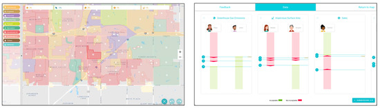
Figure 1.
Left: In iPlan, the map interface is used to change the land-use class of a given parcel, and the system computes the projected effect of the change on the selected indicators. Right: Users conduct experiments (stated preference surveys) and use a graphing tool to determine how much change the simulated stakeholders actually want.
Because the simulated stakeholders have different and often conflicting demands, users must identify and negotiate trade-offs. For example, one stakeholder may advocate for an increase in jobs, which is easiest to accomplish by re-zoning parcels for commercial or industrial use, but another stakeholder may want a decrease in greenhouse gas emissions, which will increase with commercial or industrial expansion. Thus, iPlan models not only the effects of land-use change on socio-economic and environmental indicators but also the acceptability of land-use change to various civic representatives. That is, iPlan constructs models that help people learn about the scientific and civic practices through which land-use planning is managed and contested.
iPlan was designed to integrate two effective approaches to learning. It facilitates place-based learning [24,25,26,27,28], in which learners engage in authentic problem solving situated in the place they live. Barab and colleagues [8] argue that, when learners work in a setting where they can make consequential decisions, they are more engaged in the learning activities because they believe their actions and decisions matter. Place-based curricula are thus effective because they provide consequential and realistic problem-solving activities in a location where learners are more likely to care about the consequences of their decisions [28]. iPlan enables educators or learners to choose both meaningful locations and relevant socio-economic and environmental issues to model, and it simulates authentic land-use planning practices, such as scenario construction and stated preference surveys. In this respect, iPlan also facilitates civic education [28,29] by supporting inquiry into and deliberation on public policy issues, simulating democratic and civic processes, and promoting the development of self-efficacy. Research has shown that young people with knowledge of civic issues and confidence in their deliberative abilities are more likely to take action on civic issues [29,30]. By placing learners in the role of a land-use planner interacting with community stakeholders, iPlan not only helps users understand the professional practices and civic processes of land-use planning but also to see themselves as potential stakeholders—that is, as citizens who can influence land-use decision-making.
To facilitate learning in these ways, iPlan needs to (a) construct accurate land-use maps of user-selected locations, (b) accurately model the impacts of land-use on issues that people care about, and (c) adequately simulate authentic planning practices and civic processes. In doing so, the system also needs to be accessible to educators and high-school-aged learners without expertise in land-use planning, computational simulation, or environmental modeling. As Zellner and colleagues [31] argue, there is a tradeoff “between representational fidelity and end-user intelligibility”. When models become too complex in the pursuit of more realistic representations, users become more myopically focused on understanding the model, hampering the learning and decision-making that the model is intended to facilitate. Learning gains derive less from the model itself than from the reflective and deliberative work that the model enables [32]. iPlan attempts to achieve this balance between fidelity and intelligibility for end-users who are teenagers and the educators who work with them, facilitating understanding of complex socio-environmental problems and the deliberative processes involved in addressing them while minimizing the risk that young people will regard them as problems too complex to solve.
1.2. Software Availability
iPlan version 1.0 [21] is a free, online software platform available at https://app.i-plan.us/. iPlan will run in Chrome, Safari, or Firefox on almost any laptop or desktop computer, tablet, or mobile smartphone with an internet connection.
1.3. Research Questions
To enable iPlan to construct realistic but intelligible land-use models of any location in CONUS, we developed and validated the following three primary functions: (1) the geospatial aggregation and parcelization process that divides each user-defined region into contiguous parcels and assigns a land-use class to each parcel based on geospatial land-cover data and U.S. Census data; (2) the set of land-use impact functions that quantify the effect of each land-use class on each indicator; and (3) the stakeholder threshold optimization routine that selects the minimum or maximum acceptable level that a stakeholder has for a given indicator. Collectively, these functions were designed to produce a land-use problem that is appropriately complex for high-school-aged learners, and we developed a graphical user interface that facilitates creation and use of iPlan land-use models by non-specialists.
In this paper, we focus on the following four research questions about the accuracy of these functions and the extent to which they produce land-use models that educators can use:
- RQ1. Are the land-use classifications produced by the iPlan geospatial aggregation process accurate?
- RQ2. Are the indicator values produced by the iPlan land-use impact functions accurate?
- RQ3. Do the values produced by the iPlan stakeholder threshold optimization routine match optimization targets?
- RQ4. Can educators use the iPlan system to produce land-use simulations that support their pedagogical goals and student populations?
We address each of these research questions by (a) describing our approach, (b) explaining the methods we used to assess the validity of the approach, and (c) presenting the results. We recognize that what counts as accurate, especially in reduced-form models, is highly contestable, and there are many approaches to assessing the performance of complex environmental models (see, e.g., [33]). Thus, our goal is not to show that the accuracy of iPlan models meets some a priori standard, but rather to provide evidence that the level of accuracy is acceptable given the intended uses of the system, and to provide the information that potential users need to make informed decisions about whether the platform is appropriate for their purposes. By describing in detail our modeling and game design decisions and testing the system’s performance, we hope to make transparent both the affordances and the limitations of the iPlan platform, facilitating successful use of the system in educational contexts.
2. Geospatial Aggregation and Parcelization of User-Defined Regions
2.1. Approach
The geospatial information used as the baseline data for the iPlan system was derived from the NWALT (U.S. Conterminous Wall-to-Wall Anthropogenic Land Use Trends) dataset developed by the U.S. Geological Survey [34]. The NWALT raster dataset assigns 20 land-use classes to 60 × 60 m grids. We reduced the original 20 land-use classes to 10 by removing rare or unneeded classes and consolidating similar ones (see Table A1 in Appendix A). Reducing the number of land-use classes decreases the cognitive complexity of the land-use models, making them more accessible to non-specialists, and ensures that the resulting classes can be used for the purposes of constructing land-use scenarios. For example, the original NWALT dataset includes land-use classes such as “anthropogenic other” that are potentially useful for describing existing miscellaneous land uses but make less sense as planning objectives.
After consolidating the NWALT land-use classes, we constructed four co-registered map layers at increasingly coarse scales using 2010 U.S. Census data (2020 U.S. Census data were not available at the time). Each layer contains contiguous polygons—census blocks, census block groups, census tracts, or counties—and each polygon in a layer is assigned a single land-use class. Land-use classes were assigned by selecting the class associated with the largest proportion of area in each polygon based on the underlying (reduced-class) gridded raster data. This geospatial aggregation can produce much simpler representations that retain a high degree of accuracy [35] (see Figure 2).
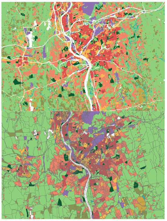
Figure 2.
Consolidated NWALT raster data (top) and the corresponding census block map layer (bottom).
To generate a land-use map of a user-defined region that has broadly accurate land-use classes but a small enough number of distinct parcels to be accessible to non-specialists, we developed a parcelization optimization routine that operates on the constructed map layers. The goal of the optimization is to produce a land-use map of the user-defined region that has no more than 200 parcels. The number 200 was chosen based on prior work [7,36,37,38], which developed land-use planning simulations in several locations, for implementation with middle- and high-school students in both formal and informal educational settings and with citizens, as part of research and outreach efforts associated with actual planning processes.
The parcelization optimization begins by comparing the selected region against each map layer. The region selected will contain either ≤200 or >200 census blocks, which is the smallest area partition. If the region contains ≤200 census blocks, the system will simply use the census blocks to construct the map, and the map may have a smaller number of parcels than the target of 200. If the region contains >200 census blocks but ≤200 census block groups (the next smallest area partition), the optimization routine will use the census block layer to construct a new parcelization. In general, the optimization routine attempts to use the nearest map layer that provides >200 polygons for the selected region.
To aggregate the >200 polygons from the nearest map layer into 200 parcels, we implement a heuristic based on minimum spanning trees and local search, which produces near-optimal solutions in very little time (typically less than 10 s). In brief, we define a parcel as a set of contiguous polygons, and we define the parcel’s land-use class as the largest class by area within the set of polygons that comprise the parcel. Ideally, the parcels that result from the aggregation of contiguous polygons will exhibit compactness: a circle- or square-like form. We want to avoid, for example, very long and narrow parcels. Our optimization routine generates 200 non-overlapping parcels which contain all the polygons present within the user-defined region. This allocation is guided by the objective of minimizing the sum of the areas of the polygons that have a different land-use class than the aggregated parcel. To ensure the compactness of each parcel, we only allow polygons from the same group in the next coarsest map layer to be combined: so, for example, only census blocks that are part of the same census block group can be combined into a parcel. (See Appendix B for more detail on the parcelization optimization routine.)
2.2. Validation Methods
Because the iPlan parcelization optimization routine only aggregates adjacent polygons with the same land-use classification in one of the pre-computed map layers, classification error in an iPlan map is equivalent to the classification error in the corresponding map layer. To assess the accuracy of the map layers that the optimization routine takes as inputs, we estimated the proportion of land area that is misallocated in the census block and census block group map layers based on the 10 consolidated NWALT classes (given in Table A1 in Appendix A).
To achieve this, we randomly selected, without replacements, 195,225 census blocks (~2% of the census blocks in CONUS) and 14,706 census block groups (~6% of the census block groups in CONUS). For each block and block group contained within the sample, we computed the proportion of area allocated to each of the 10 consolidated land-use classes based on the underlying NWALT data. We then compared these proportions to the land-use class allocated to the census block or census block group to estimate the error associated with the geospatial aggregation process.
2.3. Validation Results
Figure 3 shows the median correspondence by area between the iPlan map layers and the NWALT raster data. Parcels classed as timber in the iPlan map layers were omitted, because there were too few of them to make reliable estimates of classification accuracy.
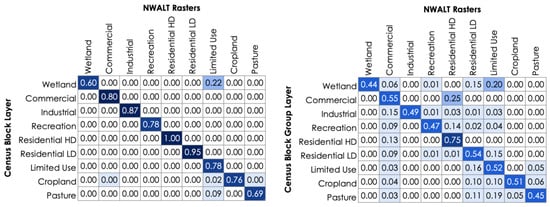
Figure 3.
Median land-use classification accuracy of the census block map layer (left) and the census block group map layer (right), relative to the consolidated NWALT data. (Residential HD = high-density residential; Residential LD = low-density residential.)
As expected, classification accuracy is highest at the census block level (Figure 3, left). Census blocks have a minimum size of 30,000 square feet, slightly smaller than the 60 × 60 m rasters in the NWALT dataset, but there is no maximum size. Because the boundaries of census blocks are determined by features (roads, railroad tracks, waterways, etc.), non-visible boundaries (e.g., school districts), special land-use areas (e.g., military bases), and governmental boundaries (e.g., county and state borders), census blocks vary substantially in size and conformation. However, half of all census blocks are less than 280,000 square feet, or approximately seven NWALT rasters. Median accuracy in the census block map layer was highest for parcels designated high-density residential (Residential HD) and low-density residential (Residential LD) (1.00 and 0.95, respectively), followed by parcels designated industrial (0.87) and commercial (0.80). This is due to the fact that these land uses tend to align well with both visible and non-visible boundaries, and they are likely to cluster (e.g., housing developments, commercial districts). Accuracy was lowest for pasture (0.69) and wetland (0.60), though in both cases, the majority of error was due to limited use land, which is a catch-all category that includes any undeveloped or minimally developed land that was not classified as one of the other categories. In other words, land-use classification at the census block level was highly accurate, and the most significant errors occurred between land-use categories with high similarities.
Classification at the census block group level is, as expected, less accurate than at the census block level, due to the coarser spatial resolution, as block groups contain more than 50 blocks on average. Median accuracy was highest for high-density residential (0.75) and lowest for pasture (0.45) and wetland (0.44). As Figure 3 shows, error was more distributed at the block group level, though as with the block level, error was largely due to similar land-use categories. For example, the most significant source of error for commercial land was high-density residential, and the most significant source of error for both pasture and wetland was limited-use land.
Table 1 provides summary statistics for each iPlan land-use category at both the census block and census block group levels, including the mean classification accuracy (proportion of area correctly classified), the upper and lower bounds of the 95% confidence interval around the mean, and the variance.

Table 1.
Statistics summarizing the accuracy of land-use classification in the census block and census block group map layers, relative to the consolidated NWALT data.
Overall, these results suggest that land-use allocation error in iPlan is within acceptable bounds for educational purposes. As Figure 4 shows, the majority of maps generated by users (58%) are less than 10,000 ha in area, and 90% of all maps created are less than 100,000 ha. That is, iPlan users generally focus on relatively small extents, so land-use classifications in the resulting maps are well aligned with local land-uses pattern.
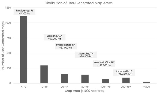
Figure 4.
Distribution of 1904 maps generated by users based on area. Cities listed in gray boxes are provided for reference purposes.
Interviews with educators who have used iPlan with learners (described in more detail in Section 5) also suggest that the land-use maps produced by the platform feel accurate to their lived experiences and those of their students.
3. Modeling the Impacts of Land Use on Indicators
3.1. Approach
The iPlan system models the impacts of 10 land-use classes on 18 indicators, including measures of air and water pollution (lead emissions, NOx emissions, particulate matter, and runoff), greenhouse gas emissions, sensible heat (added heat advisory days), wildlife populations (birds and butterflies), agricultural products (biofuels, corn, cornfed beef, and grassfed beef), structural features (housing units, impervious surface area, and green space), economic performance (jobs and sales), and population (see Appendix C for more information on the indicators).
The relationship between each land-use class and each indicator for any map in a given biome is computed using a linear equation, , where is the value of indicator contributed by land-use class , is a multiplier that characterizes the impact of each hectare of land-use class on indicator , and is the total area in hectares of land-use class in the map. The value of each indicator for the whole map, then, is given by the sum of the values of , as follows:
Thus, the key challenge is to derive the values of the multipliers , such that the relationship between a given land-use class and a given indicator in each biome is as accurate as possible, given the geographic scale and the availability of existing data and models. In most cases, each combination of indicator and land use is associated with only one multiplier, as regional variation is small enough to be insignificant, given the coarse scale of iPlan models and the prioritization of accessibility. In cases where regional variation is significant, multipliers were derived for each biome to reflect important differences in the effects of land-use in different geographic locations within the contiguous United States. (The runoff indicator was computed for groups of states, rather than biomes, because the best available dataset provided information for groups of states.) We used a variety of approaches to construct suitable multipliers (for a summary of the methods and data used, see Appendix C).
For indicators for which spatial data were available, such as jobs and housing units, we co-registered the indicator data with the census block map layer. We then computed the mean contribution of each land-use class to the indicator at a national scale to estimate the value of the indicator per hectare of each land-use class. To achieve this, we (a) downloaded spatial data from the National Historical Geographic Information System (https://data2.nhgis.org/main; accessed on 12 October 2019) and reprojected the data from the projected coordinate system (i.e., USA Contiguous Albers Equal Area Conic) to the geographic coordinate system (i.e., GCS North American 1983 High-Accuracy Reference Network); (b) co-registered the values from the National Historical GIS data with the census block map layer, which assigns a single land-use class to each census block; and (c) computed the mean value of the indicator represented in the NHGIS data per hectare of each iPlan land-use class.
For indicators for which spatial data could be imputed, such as added heat advisory days, we used PEGASUS [39] to generate spatial data. PEGASUS is a reduced-form model that estimates ecosystem photosynthesis and net production using a light-use efficiency approach combined with surface energy and soil water budgets [40,41,42,43]. The model is driven by daily data on temperature, precipitation, and potential sunshine hours. Daily data come from linear interpolation of the Climatic Research Unit monthly climatology of the global land surface at 10’ latitude/longitude resolution [44]. In addition to climate data, the model uses the International Soil Reference and Information Centre’s- WISE data on soil available water capacity [45]. For iPlan, PEGASUS was run assuming native vegetation and run again assuming complete land surface coverage with an impervious surface to simulate balances of energy and water for each land-use class. The impervious surface was parameterized by changing surface albedo, plant canopy coverage, and soil percolation constants. The simulation outputs were then combined in weighted averages according to the proportion of impervious surface area of each land-use class [46]. The process of deriving multipliers from that point was the same as that described above.
For indicators for which spatial data were neither available nor were able to be modeled at this scale, such as birds (American robins, Turdus migratorius) and butterflies (monarch butterflies, Danaus plexippus), we derived multipliers based on published findings that report relationships between indicator levels and land-uses by area (see Appendix C).
Once multipliers were computed for every combination of land use and indicator in each of the nine biomes in CONUS, we produced lookup tables that iPlan uses to compute the effects of land-use change. The results are communicated to the user in two ways: (1) in the map interface, changes in indicators are displayed as percent change from the initial value (thus, all percentages are zero for the initial map); and (2) for each submission of a land-use scenario to the virtual stakeholders, users can see the value of the indicator in its native units by accessing the data tab.
To illustrate this process in more detail, in the next section we describe how we determined the contributions of different land uses to anthropogenic greenhouse gas emissions.
Modeling the Impact of Land Use on Greenhouse Gas Emissions
Multipliers for anthropogenic greenhouse gas emissions (GHGs) were developed from a 2018 national emissions inventory [47]. This inventory was based on economic activities (e.g., shipping goods by rail), not on land uses nor on a land-area basis. To compute GHG multipliers for land-uses in iPlan, we developed a multi-step method to map the activity-based GHG emissions onto specific land uses.
The national emissions inventory breaks GHGs into five basic categories (see Table 2). These values include the emissions due to electric power generation for each category.
Table 2.
U.S. annual greenhouse gas emissions by economic sector (Table ES-7 in [47]).
First, we distributed transportation emissions into other categories, as the iPlan system does not model transportation directly. This was achieved by making a set of estimations about the types of transportation used in each of the other economic sectors (see Table 3). The majority of emissions are for personal transportation and so were allocated to the residential sector. Many of the remaining emissions involved freight transportation. Freight was considered on an “activity” basis rather than a “consumption” basis, consistent with the general method of the national emissions inventory. For example, coal freight was considered industrial because of its immediate use at a steel mill or chemical refinery, rather than being considered partly residential due to the consumption of steel or chemicals in homes. In general, freight within a vehicle type was allocated according to U.S. tonnage statistics. This assumes that the tonnage of each commodity was transported a similar distance, which may not be the case. Ton-miles would have been a better basis for allocation, but with the exception of truck freight, ton-miles statistics were not available in the necessary granularity of vehicle and commodity types. International bunker fuel use in ports (4% of total transportation emissions) was omitted due to the difficulty of attribution to the land-use types in iPlan.
Table 3.
U.S. annual transportation emissions by economic sector (vehicle type totals from Tables 3–12 in [47]).
After attribution of transportation emissions, we next addressed the sequestration of CO2 due to land management (see Table 4). In the inventory, net sequestration due to land management counts photosynthesis and ecosystem respiration but not direct emissions from fuel burning that occurs as part of land management, which is counted elsewhere. Forest land creates a significant net uptake of CO2, and human settlements also store CO2 via urban trees, soil carbon uptake from grass clippings, and organic matter in landfill. However, cropland and grassland have net emissions, due to land clearing and soil carbon loss.
Table 4.
Net GHG annual emissions due to land use (Table ES-4 of [47]).
With transportation and sequestration from land use included, the new sector totals for GHG emissions are given in Table 5. Emissions are also shown on a per-hectare basis. These were calculated by dividing sector emissions by the total area of the corresponding land-cover classes for CONUS in the NWALT dataset [34].
Table 5.
U.S. annual GHG emissions by major sector, including transportation and land-use.
With all the major CO2 sequestration and GHG emission fluxes included, we next assigned the GHG emissions from the various sectors to the land-use classes in iPlan.
The GHG emissions from the industrial and mining sectors were assigned to the iPlan land-use class industrial, commercial was assigned to commercial, and forest was assigned to timber. We separated the residential sector into the residential—HD and residential—LD land-use classes in iPlan. We achieved this using data on total household GHGs from Jones and Kammen [51]. Their study took a consumption perspective, which claims GHGs from other sectors that contribute to household consumption, including food, energy, transportation, goods, and services. Although the total GHGs attributed to residential categories by Jones and Kammen are accordingly higher than the totals in the U.S. Environmental Protection Agency (EPA) inventory, we used the ratio of high-density to low-density residential GHG emissions from their study to divide GHGs between the two residential land-use classes in iPlan. Although the ratio of high-density residential to low-density residential GHGs is slightly less than one on a per-capita basis, it is approximately 4:3 when expressed on a land-area basis. This 4:3 ratio was subsequently used to partition the inventory-based GHGs between residential land-use types.
The GHGs for the agricultural sector were similarly partitioned between the cropland and pasture land-use classes used in iPlan. The U.S. Environmental Protection Agency’s Greenhouse Gas Inventory Data Explorer [52] indicates that the total GHGs of crop and animal production in the United States are roughly equal; therefore, we assumed equal rates of GHG emissions from cropland and pasture. However, this almost certainly inflates the GHG emission rate for pasture because a significant but poorly defined proportion of animals are raised in confinement instead of pasture [53]. That said, we ignored the smaller land area of pasture relative to cropland, which deflates the pasture GHG emission rate. Because we lack the basis for more nuanced partitioning of agricultural GHGs on a land-area basis, we used one GHG emission rate for both agricultural land types (cropland and pasture), which is non-zero but far less than the emissions from industrial, commercial, and residential land uses.
All the remaining, low-use land types (limited use, wetlands, recreation) were assigned zero GHGs due to lack of inventory data that aligns with the limited-use land categories in iPlan. This assignment has the benefit of differentiating low-intensity land uses, such as parks, wetlands, and minimally developed regions, from the agricultural and forestry land classes. The final set of multipliers for GHG emissions is shown in Table 6.
Table 6.
GHG emission multipliers used in iPlan.
Two caveats about the GHG multipliers should be noted. First, since inventory GHGs are due to human activity and mostly to fossil fuel combustion, the multiplier values were assumed to be independent of biome. Therefore, only one GHG multiplier per land use type was created for all of CONUS, even though the net sequestration values from agriculture, forestry and human settlements do vary across regions. Second, the EPA inventory values are for the entire United States, not just CONUS. However, Alaska and Hawaii together comprise just 1% of U.S. energy-related emissions [54], so the U.S. emissions were used to approximate CONUS emissions.
3.2. Validation Methods
To validate this process, we compared the outputs of the iPlan GHG emissions equations, which are land-use based, to values contained in the Vulcan Project’s annual emissions data [55], an inventory-based dataset that was not used to derive the iPlan multipliers. The Vulcan dataset provides GHG emissions values for all locations in CONUS at 1 km spatial resolution and is in good agreement with GHG emissions calculated from atmospheric samples [56]. The Vulcan authors intend the data for use by municipalities to calculate their own GHG emissions, in lieu of expensive self-inventories, and thus Vulcan data are presented at a relevant spatial resolution for iPlan.
Vulcan presents annual (2010–2015) GHG emissions from combined fossil fuel combustion and cement production, which is abbreviated “FFCO2”. Vulcan includes information on combustion economic sector (e.g., on-road, residential, electricity, or airport), combustion subsector (e.g., vehicle class or building type), combustion process (e.g., boiler, turbine, or engine), and fuel description (e.g., individual petroleum fuels or coal grade). Although the dataset is gridded, the underlying data were individual point, line, and polygon source elements chosen and processed to represent census block-group sizes or finer. The “spatialization” of FFCO2 onto a 1 km grid was undertaken using federal datasets produced by the Federal Emergency Management Association, the Department of Energy, the Federal Highway Administration, the EPA, and others.
Our GHG validation exercise compared FFCO2 from the year 2015 to iPlan GHG emissions output at three different spatial scales: 300 × 300 km, 30 × 30 km, and 3 × 3 km. Locations across CONUS were randomly selected for each spatial scale, with 1661, 585, and 122 sites chosen at the 3 km, 30 km, and 300 km scales, respectively. Bodies of water were excluded from the analysis. At the randomly chosen sites, the sums of FFCO2 and GHG emissions were computed for the sample area, and then Pearson’s correlations between the set of FFCO2 and GHG sums were calculated for each of the three scales. It should be noted that total U.S. GHG emissions are somewhat larger than FFCO2 since GHGs include fluxes from agriculture and land-use change.
3.3. Validation Results
Figure 5 shows the correlations between the inventory-based FFCO2 emissions in the Vulcan dataset and the land-use-based GHG emissions computed in iPlan at three spatial resolutions.
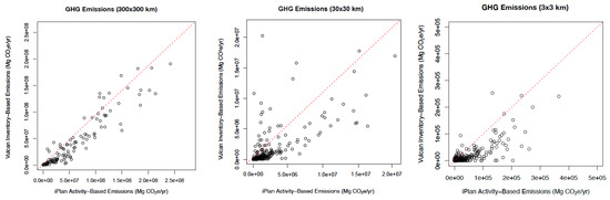
Figure 5.
Correlations between the inventory-based GHG emissions in the Vulcan dataset (y-axis) and the land-use-based GHG emissions computed in iPlan (x-axis) at three spatial resolutions.
At the coarse spatial resolution (300 × 300 km), there is a high correlation (Pearson’s r = 0.95) between the Vulcan data and the iPlan system’s computed GHG emissions. This indicates that iPlan is accurately computing the overall load of GHG emissions. As expected, the correlation decreases substantially with increasing spatial resolution: for 30 × 30 km samples, Pearson’s r = 0.72, and for 3 × 3 km samples, Pearson’s r = 0.20. iPlan consistently computes higher GHG emissions values than those in the Vulcan dataset, in part because the assignment of GHG emissions from power plants and transportation in iPlan is distributed to other land-use classes, such as residential and commercial. For example, iPlan models the fact that electricity demand in households and businesses is the primary cause of GHG emissions at power plants. Samples with smaller areas are less likely to include power plants, and therefore there is greater divergence between the Vulcan values and the iPlan outputs with increasing spatial resolution.
4. Optimization of Stakeholder Preferences
4.1. Approach
A key feature of iPlan simulations is the ability, not only to model the impacts of land use on various indicators, but also to construct land-use scenarios for submission to virtual stakeholders who provide feedback on proposed land-use changes. Because each land-use model created by the iPlan system is a unique result of user selection and non-deterministic optimization, the preferences of the virtual stakeholders need to be set automatically, such that the resulting land-use problem space is neither too simple nor too complex. To achieve this, we constructed a large set of stakeholders, assigned one indicator to each stakeholder, determined whether they would advocate for that indicator to be above or below some threshold, and then developed an optimization routine to set the thresholds such that the resulting land-use problem would have an appropriate level of complexity.
In iPlan, a land-use model includes nine virtual stakeholders, each of whom advocates for land-use based on one indicator. Thus, because each model includes five indicators, there are two stakeholders who care about four of the indicators, and one stakeholder who cares about the fifth. The nine stakeholders are representatives of three fictitious groups: the Local Business Consortium, the Environmental Justice Center, and the Community Coalition. These groups were designed to reflect the three largest constituencies in planning processes: business leaders and owners, environmentalists, and residents.
We constructed 54 virtual stakeholders, each of whom has a name, image, job, brief biography, stakeholder group, and indicator. We developed 54 so that each of the 18 indicators is associated with one member from each of the three stakeholder groups. For each stakeholder, we also determined whether they prefer their assigned indicator to be above or below some threshold. For every indicator, there is at least one stakeholder who desires it to be below a threshold and at least one who desires it to be above a threshold, which models the fact that different constituencies have different goals. For example, a business lobby may advocate expanding commercial or industrial development to increase jobs and revenue, while homeowners may oppose such expansion due to the increased traffic, pollution, or noise.
The system selects the nine stakeholders for each land-use model based on the indicators chosen and a prioritization algorithm, then the system runs an optimization routine to set the indicator threshold for each stakeholder. This process is explained in detail in Appendix D. The objective of the optimization is to set the thresholds, such that the distribution of land-use scenarios that satisfy some number of stakeholders matches a target distribution. The default target distribution (see Figure A1) is based on prior work developing land-use simulations for use by high-school and adult learners [7,36,37,38], but a key advantage of this approach is that the difficulty of iPlan simulations can be adjusted simply by adjusting the target distribution.
Because there are 11200 possible land-use scenarios that can be constructed for a given land-use model, we use a sampling process to generate a set of reasonable land-use scenarios for that model, which in turn generates distributions of indicator values from which to select and optimize threshold levels. There are two constraints on this optimization, as follows: (a) no more than four stakeholders can be satisfied with the initial map produced by the parcelization process, and (b) two stakeholders assigned the same indicator cannot have the same threshold.
4.2. Validation Method
To validate the stakeholder threshold optimization routine, we randomly selected 6000 rectangular extents with diagonals of approximately 10 km. Each extent was processed using the parcelization optimization routing, to create 6000 extents with 200 parcels each. For each extent, five indicators were randomly selected, and then the stakeholder threshold optimization routine was applied.
4.3. Validation Results
Figure 6 shows the correspondence between the output of the stakeholder threshold optimization routine and the target distribution, which indicates that the optimization process can reliably produce stakeholder thresholds that approximate the target distribution.
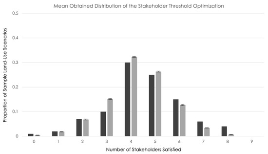
Figure 6.
Histogram showing the target distribution (dark grey) and the mean obtained distribution with 95% confidence intervals produced by the stakeholder threshold optimization routine (light grey). The height of the bars represents the proportion of sample land-use scenarios that satisfy each number of stakeholders.
This result also suggests that adjusting the target distribution could provide a useful mechanism for controlling the difficulty of the land-use simulations that iPlan produces.
5. Use of the iPlan Platform in Educational Contexts
To integrate all the modeling features of iPlan into a usable simulator, we developed an ArangoDB graph database for storing the geospatial data. By indexing all the parcels in every map layer and precomputing their locations and adjacencies, we can run the parcelization optimization routine in a matter of seconds. To develop the software application, we used the Ionic platform. Ionic is an HTML5 (HyperText Markup Language version 5) mobile application development framework for building hybrid mobile apps (small websites running in a browser shell as an app that can mimic native apps). Unlike pure native apps, hybrid mobile apps are faster to develop and deploy and can function on a broader range of platforms. This enables iPlan to run on any platform with an Internet browser, including laptops, Chromebooks, tablets, and mobile phones.
A key affordance of this approach is that users can construct land-use simulations in iPlan and share them with other users. For example, educators can construct a land-use simulation and share it with learners, so that all learners are using identical simulations to construct their land-use scenarios. This process involves simply sharing a URL, and anyone who logs in to iPlan using that URL will have access to that model. However, each user will have their own copy of the model; the current version of iPlan does not support collaborative use.
At the time of this writing, more than 2000 individuals have used iPlan to construct and explore land-use models of regions in 40 U.S. states. Educators have successfully constructed and used iPlan models in a variety of subject areas and learning contexts, including in units on water quality, urban planning, sustainable cities, ecological restoration, human geography, and general biology. The following examples illustrate three ways educators have integrated iPlan into their curricula and provide preliminary evidence that they are able to use iPlan to achieve their educational goals.
5.1. Example Uses of iPlan in Classroom Contexts
5.1.1. Introduction to Science, Technology, Engineering, and Math (STEM) Disciplines and Careers
At a high school with a predominantly Black and Latine student population in Pawtucket, Rhode Island, iPlan is part of a class designed to introduce 9th-grade students to STEM disciplines and the social impacts of STEM professionals. For the climate science and land-use planning unit, the teacher begins with lessons on greenhouse gases, the carbon cycle, and the ozone layer, then uses iPlan to help students understand how land-use planning can address environmental challenges like the greenhouse effect but that there are trade-offs in doing so. At the beginning of the simulation, students often expressed a sense of hopelessness: “Can we ever get to net zero?” or “Did you give us this assignment so you could stress us out? Nobody can be happy”. But by the end, she said, “students felt more confident that there are things that can be done”. They recognized the challenges and tradeoffs involved, but they also saw how those challenges and tradeoffs could be addressed.
One of the teacher’s goals for the unit was to have more grounded conversations with students about how land-use planning works. Specifically, she wanted them to see that they could have a voice in land-use planning processes: “I wanted students to have a better appreciation of the range of stakeholders … even to the point where they could see that they could be stakeholders. … It’s not just to beat the game, pleasing people … but these are people in the real world and you could have a say in this”. While iPlan places the user in the role of a planner, not a stakeholder, the virtual stakeholders were constructed to represent a broad range of people, with various appearances, backgrounds, and social roles, to help learners see that stakeholders are simply “people in the real world”.
The teacher also felt that it was important to link STEM professional activities to social impacts in their community. During one semester, the unit took place during a heat wave, prompting a conversation about the relationship between land-use and extreme heat in the context of climate justice. Another time, the class discussed a strip mall down the street from the school that was being redeveloped, and specifically, the process through which such development happens: “Before anyone builds they have to go to the zoning board. There’s a group of people making these decisions. They can’t just plop a business down in a housing neighborhood”. Overall, the teacher felt that the simulation helped her students understand both the relationships between land-use and environmental or socio-economic issues and the civic process of land-use planning.
5.1.2. Life on Earth, Localized
At an underfunded high school in rural Massachusetts, iPlan is part of a “Life on Earth” class for 11th- and 12th-grade students. The teacher uses iPlan in a unit on land-use planning to learn about planning practices, explore multi-objective problems with no perfect solution, experience the challenge of representing diverse perspectives, and understand quality indicators. The teacher sees the class as an important way to engage disenfranchised students, noting that it “keeps kids coming back to school”.
One of the advantages of iPlan, she noted, is that it is the “only opportunity students have where they have to represent other people. … They aren’t a player, they don’t have an avatar”, which “focuses them on the stakeholders”. It was important to her that the students not only learn about the relationships between land use and the environment but also that civic processes often involve negotiating among competing priorities. For example, in one semester, she had her students use a simulation of a neighboring town, a formerly successful industrial area “where there are a lot of closed mills”. She had them focus on increasing jobs in the area but wanted them to recognize how re-industrialization can also lead to environmental harms. It successfully stimulated conversations on tradeoffs and the challenges involved in solving multi-objective problems.
The teacher also incorporated the town’s actual planning work into the class, as the town is currently considering proposals for redevelopment of the site of a former state institution that is walking distance from the school. The town planner visited the class, and after using iPlan, the students produced a plan for the site and an accompanying vision statement to help them understand one way that young people can engage in civic decision-making; they were familiar with other towns that are “struggling and fading, … they know what happens when there isn’t a coordinated effort by people who care”. The teacher then submitted the proposals of willing students to the local planning board. The first time she brought student proposals to the planning board, the members “were absolutely floored [that students] were actively engaged in the planning process”. iPlan provided “a direct link between … school learning and this very important project that has the potential to influence … [our town] for decades to come”. When she told her students how the planning board reacted to their proposals, “there was a lot of blushing going on. … They were really proud”.
5.1.3. Field Biology
At the largest high school in New Hampshire and the public high school for six small towns, iPlan is used as part of a “Field Biology” elective. In the “Freshwater” unit, students learn about runoff and pollution, conduct water quality tests of a nearby lake, and then use iPlan in the same location as their testing site. The class is visited by the town planner, and then they use iPlan to try to improve the health of the lake while also accommodating a growing population. “They know the health of the lake is not great, so they do not want to do anything [in iPlan] to make it worse”. iPlan helps interest the students in the way land-use planning can be used to address the effects of climate change, such as warming temperatures leading to declining water quality in the lake, which is an important part of the local ecology and economy.
Like other educators, the teacher reported that iPlan works well for students who do not respond well to more traditional curricula. “Every student was engaged, even my students who always put their heads down”, because they could take meaningful action on issues that otherwise felt remote and unchangeable. One of the boys “who usually doesn’t do anything [in class]”, she explained, even started using iPlan on his own just to see the land-use maps of other locations. She also saw iPlan as a useful tool for helping students to support one another’s learning. Students often talk while they play, sharing information: “One kid would say, ‘I can’t make so-and-so happy’ and then another would say ‘trying changing X to Y’ … or “if you change this to that, the birds go way down”.
5.2. Summary of Educators’ Experiences with iPlan
Feedback from educators (N = 19) is being collected using a semi-structured interview protocol and survey. While the number of survey responses is currently too low for meaningful quantitative analysis, which will be conducted in a future study, preliminary qualitative analysis indicates broad agreement from educators that iPlan (a) produces realistic, accessible land-use models that are easy to use; (b) supports learning about the relationship between land-use and indicators, multi-objective problems with diverse solutions, the challenge of representing diverse perspectives, and the ways in which scientific and civic practices are interrelated; (c) works well with a range of learners, and in particular with learners who are not engaged by more traditional learning modalities; and (d) facilitates engagement with real-world planning processes. As one teacher from Boston summarized it:
The iplan tool is a very realistic modeling tool. It was easy to use for both me and my students, and allowed each student to engage with the model at their own level. I loved the fact that we could model our community—I have been struggling to find ways to teach about ecological restoration, and its implications at the local level, that shows kids real world applications, and this tool really helped me do that. My students really buy into learning more when the topic at hand relates to where they live, play, and go to school.
While all educators interviewed to date offered suggestions for improvement or requested additional features, they agreed that the platform addresses their educational needs by providing learners with realistic, localized land-use models in an authentic simulation of scientific and civic land-use planning practices.
These findings are in alignment with previous studies of iPlan usage. For example, the Massachusetts Audubon Society and Rhode Island Environmental Education Association conducted a pilot study [57] with 10 high-school teachers who implemented iPlan in 24 sessions with 321 students (a total of 2185 contact hours). All 10 teachers reported that iPlan was “easy to use,” and 9 out of 10 reported that they could integrate iPlan simulations into future classes. The study also surveyed students (N = 281) about their experience using the simulations. Fifty-three percent reported that the simulation was “easy to use” (only 20% reported that it was not easy to use); 56% reported that it was “fun to use” (only 18% reported that it was not fun to use); and 63% reported that they “were focused while using iPlan” (only 12% reported that they were not focused). In other words, both teachers and students reported a positive user experience, and the primary finding was that teachers need more support integrating iPlan effectively into their curricula. To that end, the Rhode Island Environmental Education Association is currently developing curriculum units that provide wrapper activities and professional development supports for teachers, and other curriculum units have been developed to help teachers use iPlan more effectively [58].
6. Discussion
In this paper, we described iPlan, a free, online software application that enables educators and learners to easily create and implement custom land-use simulations of any location in CONUS. Learners can use iPlan simulations to construct land-use scenarios, see the effects of land-use change on environmental and socio-economic indicators, and explore how simulated stakeholders respond to proposed changes as they attempt to devise land-use plans that satisfy as many stakeholders as possible. We presented evidence that the three primary computational models—which produce parcelized land-use maps of user-defined locations, calculate the local effects of land-use change on various indicators, and set stakeholder priorities—are sufficiently accurate for educational purposes. Moreover, initial interviews with educators indicate that (a) the system creates realistic representations of local conditions, (b) educators can construct simulations that meet their curricular and pedagogical needs, and (c) iPlan is an effective educational technology, especially for learners less motivated by more traditional curricula.
As with any model, and especially with reduced-form models, there is no standard way to determine what counts as “accurate enough” for the intended purposes. However, by describing our modeling methods in detail and systematically testing model performance against known standards, we demonstrated that iPlan achieves its modeling goals, and we provide information that enables potential users to determine if the software will meet their needs.
There are, of course, many important factors that iPlan does not account for when simulating the effects of land use on environmental and socio-economic indicators, including transportation, adjacency effects, and temporality. Because the software needs to be accessible to educators and learners, the system excludes these and other relevant factors to make the problem space more tractable and to help learners understand basic relationships between land use and issues that people care about. However, in future versions, we plan to incorporate several additional functionalities based on feedback from educators, including (a) modeling the effects of land-use change under a set of assumptions about how climate change will affect the selected location; (b) modeling the effects of land-use change broken out by demographic categories and spatially distributed based on properties of the selected location; and (c) modeling the effects of land-use adaptations, such as shade tree planting, construction of flood barricades, and solar panel installation, on select indicators. While this will present challenges for accessibility, we believe these can be addressed by optimizing the number of parcels included in the land-use map, the number of indicators and land-use classes/modifications included in the simulation, the number of demographic categories and other data layers included in the model, the difficulty of satisfying the virtual stakeholders (i.e., the target distribution used to set stakeholder preferences), or the number of stakeholder feedback requests allotted (this is the means of modulating the tractability of current iPlan simulations).
A key finding of user experience testing to date is that educators need more support for integrating iPlan effectively into their curricula, including professional development and suggested wrapper activities that supplement or enhance the activities in the iPlan system [57,58]. This work is ongoing and will be described in a future paper. However, it points to a key challenge in the design of learning systems more broadly, namely that the flexibility of customization requires different skills from educators to successfully utilize them [59]. This will involve developing and testing new models of professional development and further development of the platform itself to more effectively guide educators on its use.
In addition, further research is needed on how iPlan improves learning. As we argue elsewhere [60], the more customizable an educational experience is, the more difficult it is to design learning analytic models or assessment systems that can be reliably used to measure learning. In other words, constructing normative assessments of learning in complex learning environments when neither the content nor the context is standardized presents significant challenges [61]. Indeed, the very features of iPlan that make it appealing to educators—namely, the features that facilitate customization of the location and socio-environmental issues modeled—mean that each simulation an educator creates is unique. Moreover, iPlan was designed to be a tool, not a curriculum, and, thus, teachers use it in a range of ways, as the examples described in Section 5 indicate. While there are many validated measures of relevant constructs, for example, environmental literacy, there is no reason to expect that those measures would be appropriate for any given use of iPlan, and, because different educators use different simulations, there would be no way to aggregate or compare different cases even if such a measure could be used. Thus, we have relied on qualitative methods to assess the effectiveness of iPlan, and this work is ongoing, and we are currently developing methods to assess learning quantitatively in the absence of normative assessments [60].
While iPlan was designed for and is primarily used in educational contexts, it may also be useful as a decision support tool. For example, the Capital Area Regional Planning Commission, in Dane County, Wisconsin, used a prototype version of iPlan to better understand the land-use decisions that citizens would make to address the related challenges of expanding population and water conservation [37]. They found that, when asked, citizens generally favored infill and multi-family dwellings as a solution to anticipated population growth, but when presented with an interactive land-use simulation, the same individuals were more likely to add housing to peripheral land currently undeveloped or used for agricultural or recreational purposes. That is, people articulated an imperative to maintain a smaller development footprint but struggled to actually implement it, even in a simulation. Using the simulation thus enabled the planning commission to have more grounded conversations with stakeholders about how to address future growth in the area.
iPlan is thus a flexible platform that both young people and adults can use to explore how land use affects local issues—and how changes in land-use patterns can address a range of pressing environmental and socio-economic challenges.
Author Contributions
Conceptualization, A.R.R.; methodology, A.R.R., C.B., J.B., Y.T. and D.W.S.; validation, A.R.R., C.B., Z.C. and Y.T.; formal analysis, A.R.R., C.B., Z.C. and Y.T.; data curation, M.B. and T.J.L.; writing—original draft preparation, A.R.R. and C.B.; writing—review and editing, A.R.R., C.B. and J.B.; supervision, A.R.R., T.J.L. and D.W.S.; project administration, A.R.R. and D.W.S.; funding acquisition, A.R.R. and D.W.S. All authors have read and agreed to the published version of the manuscript.
Funding
This work was funded in part by the National Science Foundation (DRL-1713110), the Wisconsin Alumni Research Foundation, and the Office of the Vice Chancellor for Research and Graduate Education at the University of Wisconsin-Madison. The opinions, findings, and conclusions do not reflect the views of the funding agencies, cooperating institutions, or other individuals.
Institutional Review Board Statement
The study was conducted in accordance with the Declaration of Helsinki, and approved by the Institutional Review Board of the University of Wisconsin–Madison (2014-0823, approved 14 July 2014, and 2021-0675, approved 9 July 2021).
Informed Consent Statement
Informed consent was obtained from all subjects involved in the study.
Data Availability Statement
The datasets presented in this article are not readily available because they are part of ongoing research. Requests to access the datasets should be directed to the corresponding author.
Conflicts of Interest
The authors declare no conflict of interest.
Appendix A. Land-Use Data Preparation
Appendix A.1. Land-Use Class Consolidation
Table A1 gives the original NWALT land-use classes and the corresponding classes in iPlan. We removed pixels classed as “Water” (class 11), as those cannot in most cases be changed to anything else, and we removed pixels classed as “Major Transportation” (class 21) because the inclusion of transportation would have made the resulting land-use models too complex for non-specialist users. We also removed pixels classed as “Very Low Use, Conservation”, which are very rare—to the point where the class virtually disappears from the census block map layer—and, in many cases, represent land uses that are not generally changeable, such as national historical markers. The remaining 17 NWALT classes were consolidated into 10 classes by aggregating land uses with similar compositions and socio-economic and environmental impacts.
Table A1.
Reduction of 20 NWALT land-use classes to 10 iPlan land-use classes.
Table A1.
Reduction of 20 NWALT land-use classes to 10 iPlan land-use classes.
| NWALT Land-Use Class | iPlan Land-Use Class |
|---|---|
| 11. Water | Removed |
| 12. Wetlands | Wetlands |
| 21. Major Transportation | Removed |
| 22. Commercial/Services | Commercial |
| 23. Industrial/Military | Industrial |
| 24. Recreation | Recreation |
| 25. Residential, High Density | Residential—High Density |
| 26. Residential, Low–Medium Density | Residential—Low Density |
| 27. Developed, Other | Commercial |
| 31. Urban Interface High | Limited Use |
| 32. Urban Interface Low Medium | Limited Use |
| 33. Anthropogenic Other | Limited Use |
| 41. Mining/Extraction | Industrial |
| 42. Timber and Forest | Timber |
| 43. Cropland | Cropland |
| 44. Pasture/Hay | Pasture |
| 45. Grazing Potential | Pasture |
| 46. Grazing Potential Expanded | Pasture |
| 50. Low Use | Limited Use |
| 60. Very Low Use, Conservation | Removed |
In response to feedback from educators, we then added an additional land-use class, “Conservation”, so that users of iPlan can designate a parcel as conservation, even though it will never appear on initial maps constructed by the system. For the purposes of modeling, conservation behaves identically to limited use. Table A2 provides a brief definition of each iPlan land-use class, based on both the consolidated NWALT classes and the ways in which the land uses are modeled in iPlan (see Appendix C).
Table A2.
Definitions of the land-use classes in iPlan.
Table A2.
Definitions of the land-use classes in iPlan.
| Land-Use Class | Definition |
|---|---|
| Commercial | Commercial land is primarily used for services or businesses, including shopping centers, office buildings, retail shops, schools, hospitals, churches, prisons, and police and fire stations. |
| Conservation | Legally designated conservation lands constrain or prohibit development. While conservation land can be privately or publicly owned, it is typically characterized by very low or no human usage. Conservation objectives may include goals like water quality management, the maintenance or restoration of wildlife habitats, or supporting sustainable agriculture or forestry. |
| Cropland | Cropland produces foods for humans and animals, as well as raw materials for textiles, biofuels, and many other consumer goods. Corn is the most widely grown crop in the United States, accounting for more than 90 million acres of land, and the majority is grown for livestock feed. |
| Industrial | Industrial land is used mainly for the extraction of natural resources or the production, storage, and shipment of commodities. Rock quarries, mines, and energy operations extract and refine raw materials, and factories, workshops, and production plants create materials, components, and finished products. Military installations, waste processing facilities, and seaports are also considered industrial. |
| Limited Use | Limited use regions have low or no human usage or impact. These areas can include rural and sparsely populated exurban communities (<16 housing units/km2), unmanaged green space and unused lots, mountains and deserts, as well as Superfund sites or other areas inhospitable to human habitation. |
| Pasture | Pasture, which includes grasslands and prairies, is undeveloped or minimally developed land dominated by grass and herbaceous vegetation. Pasture is land actively used for livestock grazing or the production of seed or hay crops, or land with the potential for such use that has a housing unit density <124 units/km2, is not on a military base or part of protected land such as a national park, has a grade of <30%, and is within 1 km of water. |
| Recreation | Recreational land includes areas commonly used for entertainment purposes, including golf courses, playgrounds, open sports arenas and playing fields, racetracks, amusement parks, and zoos. |
| Residential—HD | High-density residential areas have a housing unit density of >500 units/km2. These areas typically include multi-family residences, like apartments and condominiums, which house multiple families in a single structure, as well as neighborhoods of closely built single-family homes. |
| Residential—LD | Low-density residential areas have a housing unit density of 16–500 units/km2. These areas typically include residences that house one or two families per structure that are distributed over larger areas than high-density residential areas. |
| Timber | Timberlands are undeveloped regions dense with trees. These areas have a housing unit density < 10 units/km2, are not on or near a road, and are outside the borders of cities. |
| Wetlands | Wetlands are regions that are either permanently or seasonally flooded with water. |
Appendix A.2. Map Layer Construction
To construct each of the four map layers (census block, census block group, census tract, and county) and allocate a land-use to each polygon, we performed the following four steps using the arcpy, postgresql with the postgis extension, and/or pandas software packages:
- Reprojection. We reprojected the GIS data for each layer from a projected coordinate system (USA Contiguous Albers Equal Area Conic) to a geographic coordinate system (GCS North American 1983 HARN) to co-register the census data with the NWALT data.
- Land-use allocation. To assign a land-use class to each polygon, we identified the iPlan land-use class (see Table 1 above) in the NWALT raster data that accounts for the most area in a given polygon (e.g., a given census block). We then assigned that land-use class to the entire polygon.
- Computation of basic spatial parameters. We calculated the area of each polygon in each map layer, as well as the latitude and longitude of the centroid of each polygon.
- Adjacency table generation. We generated adjacency tables based on geographic adjacency among polygons. The record for each polygon also indicates to which polygon in the next coarsest map layer it belongs. For example, the record for each census block indicates which census block group it belongs to.
This process produced the map layers on which the parcelization optimization routine operates.
Appendix B. Parcelization of a User-Defined Region
Parcelization of a user-defined region is accomplished using an optimization routine that operates on the map layers. To aggregate the >200 polygons from the nearest map layer into 200 parcels, we implement a heuristic approach.
Adjacency among polygons in a given map layer (i.e., adjacency among census blocks, census block groups, etc.), is represented by an undirected graph, , where the set of vertices V is defined by the centroids of the set of polygons, and there is an edge, , between adjacent polygons. A parcel is a connected subgraph of . The problem of obtaining disjoint connected subgraphs of an undirected graph is a particular case of the so-called spatial unit allocation problem [62,63,64]. Spatial unit allocation aims to allocate spatial units to different regions while respecting some allocation criteria. The most common criteria are contiguity and compactness, which are both included in our optimization.
Given a graph , we define as the set of all possible parcels, as the set of vertices in parcel . The cost of a parcel is defined as the total mismatched area in the parcel.
In our heuristic approach, the edges of graph receive a weight based on the area of the vertices they connect and whether their land use is the same or not. By obtaining the minimum spanning tree of this weighted graph, we are able to rapidly identify parcels with low cost. This approach, which is combined with local search, gives near-optimal solutions with minimal computation time, making this heuristic well suited for an online application.
Appendix C. Indicators Included in the iPlan System
iPlan includes 18 indicators, which are given in Table A3. These indicators represent a range of social, economic, and environmental phenomena that can be reasonably modeled using only location and land-use information as inputs.
Table A3.
The 18 indicators included in iPlan.
Table A3.
The 18 indicators included in iPlan.
| Indicator | Definition | Units | Region-Specific | Model/Data Source |
|---|---|---|---|---|
| Added heat advisory days | Days per year when the heat index is ≥100 °F for at least 2 h | Days per year | Yes | PEGASUS [39] |
| Biofuels | Energy potential of fuel-grade ethanol that can be produced from corn, under the assumption that all cropland is used for corn production | 10,000 kilocalories per year | Yes | PEGASUS [39] Hay [65] |
| Birds | American robins (Turdus migratorius) | Total number | Yes | PEGASUS [39] North American Breeding Bird Survey (https://www.pwrc.usgs.gov/bbs/; accessed on 10 September 2018) Blair [66] |
| Butterflies | Monarch butterflies (Danaus plexippus) | Total number | Yes | PEGASUS [39] Pleasants [67] Thogmartin et al. [68] |
| Corn | Food energy of corn produced for human consumption, under the assumption that all cropland is used for corn production | 10,000 kilocalories per year | Yes | PEGASUS [39] FoodData Central (https://fdc.nal.usda.gov/index.html; accessed on 15 July 2018) |
| Cornfed beef | Food energy of beef produced from cows that primarily eat corn products, under the assumption that all cropland is used for corn production | 1000 kilocalories per year | Yes | PEGASUS [39] “On Average, How Many Pounds of Corn Make One Pound of Beef?” [69] |
| Grassfed beef | Food energy of beef produced from cows that primarily eat grass and other forage, under the assumption that all pasture is actively grazed by cattle | 1000 kilocalories per year | Yes | PEGASUS [39] Penman et al. [70] |
| Green space | Proportion of non-impervious surface area (e.g., forest, grassland, wetland, etc.) | Percentage of non-impervious surface area | No | NWALT [34] |
| Greenhouse gas emissions | Emission of carbon dioxide, methane, and other greenhouse gases into the atmosphere | Metric tons of carbon dioxide equivalents per year | No | Hockstad and Hanel [47] Jones and Kammen [51] Kellogg [53] Kuhle and Sloan [50] Greenhouse Gas Inventory Data Explorer [52] U.S. Travel Answer Sheet [49] Worth et al. [48] |
| Housing units | Estimated number of housing units (number of housing units in the 2010 U.S. Census plus estimated new residential construction and estimated new mobile homes minus estimated housing units lost) | Number of housing units | No | National Historical Geographic Information System (https://data2.nhgis.org/main; accessed on 20 March 2017) |
| Impervious surface area | Proportion of impervious surface area (e.g., concrete, asphalt, structures, etc.) | Percentage of impervious surface area | No | NWALT [34] |
| Jobs | Number of employed persons, including full- and part-time employment and self-employment | Number of jobs | No | National Historical Geographic Information System (https://data2.nhgis.org/main; accessed on 14 May 2017) |
| Lead emissions | Emission of lead into the atmosphere | Grams per year | No | 2014 National Emissions Inventory (NEI) Data (https://www.epa.gov/air-emissions-inventories/2014-national-emissions-inventory-nei-data; accessed on 18 August 2019) |
| NOx emissions | Emission of nitrogen oxides (NOx) into the atmosphere | Kilograms per year | No | 2014 National Emissions Inventory (NEI) Data (https://www.epa.gov/air-emissions-inventories/2014-national-emissions-inventory-nei-data; accessed on 20 September 2019) |
| Particulate matter emissions | Emission of particulate matter (PM2.5) into the atmosphere | Kilograms per year | No | 2014 National Emissions Inventory (NEI) Data (https://www.epa.gov/air-emissions-inventories/2014-national-emissions-inventory-nei-data; accessed on 25 September 2019) |
| Population | Estimated number of people (number of people in the 2010 U.S. Census plus births and migrations minus deaths) | Number of people | No | National Historical Geographic Information System (https://data2.nhgis.org/main; accessed on 27 April 2018) |
| Sales | Gross sales per year | Dollars per year | No | (Adopted from a prior version of the iPlan modeling system: Bagley and Shaffer [71]) |
| Runoff | Flow of unabsorbed water | Metric tons per year | Yes * | Water Erosion on Cropland, by Region and Year (https://www.nrcs.usda.gov/wps/portal/nrcs/detailfull/national/technical/nra/nri/results/?cid=nrcs143_013656; accessed on 10 October 2019) Franzmeier and Steinhardt [72] Wischmeier and Smith [73] |
* Unlike the other region-specific indicators, which vary by biome, runoff varies by groups of states.
Appendix D. Assignment of Stakeholder Preferences
To set the thresholds for stakeholder preferences in iPlan land-use models, the system selects nine stakeholders with pre-defined indicator directionality preferences—that is, whose preference for their assigned indicator is either above or below some threshold—and an optimization routine determines the threshold for each stakeholder, based on the properties of the parceled land-use map produced by the iPlan system.
Let denote the area assigned to each of land-use classes. Let denote the multipliers on the land-use classes for the indicator . Then, for a given map, the indicator values for indicators are computed by the following:
When the land-use class assignment is changed in one or more parcels, the total area of at least two land-use classes is changed, and the indicator values are recomputed. For a given map with parcels and land-use classes, the total possible number of land-use scenarios is (in the current version of iPlan, 11200).
For a given land-use model, the difficulty of developing satisfactory land-use scenarios can be approximated by the proportion of all possible land-use scenarios that satisfies exactly zero, one, two … nine stakeholders. Because there are more possible land-use scenarios for a given iPlan model than there are atoms in the universe, this probability distribution can only be estimated. The objective of the optimization is to set stakeholder thresholds such that the (estimated) probability distribution for the model matches a target distribution. We currently use the target distribution shown in Figure A1, but other distributions could be chosen to adjust the difficulty of developing satisfactory land-use scenarios. Note that the value for satisfying all nine stakeholders is zero, which reflects the fact that it is virtually impossible to satisfy everyone in a land-use planning process.

Figure A1.
Probability distribution used as the target for optimizing stakeholder preference thresholds.
Appendix D.1. Land-Use Scenario Sampling
To estimate the probability distribution of stakeholder satisfaction for a given land-use model, we first implement a sampling algorithm. For a given map with parcels and land-use classes, we randomly generate land-use scenarios under the following constraints:
- No more than 10% of the parcels may be changed to a new land-use class;
- The number of parcels changed is a random variable with a normal distribution with and ;
- The area of any changed parcel cannot exceed 50% of the total map area;
- The area of any changed parcel is a random variable with a normal distribution with , where is the total area of all parcels.
Under these four constraints, we draw a random sample of scenarios with size . The following algorithm is used to produce one land-use scenario:
- Choose a random number, , from a normal distribution with and , restricted to the range This is the number of parcels whose land-use class will be changed.
- Find the parcel, , whose area is closest to a random number, , drawn from a normal distribution with , restricted in the range where is the total area of the map.
- Assign a new, randomly selected land-use class to the selected parcel.
- Repeat steps 2 and 3 until parcels have been changed.
This process is repeated until scenarios are generated. In the current version of iPlan, .
Appendix D.2. Computing the Indicator Values for the Land-Use Scenario Sample
Once we have generated a large set land-use scenarios using the conditional random sampling procedure described above, we compute the indicator values for each scenario.
For a given land-use scenario , we sum the parcel areas, , for each land-use class. This produces a vector , where is the total area of the parcels with land-use class . These vectors form a matrix, . For indicators, each of which has a multiplier, , for each land-use class, the multipliers form a matrix, as follows:
where is the multiplier for indicator and land-use class . The indicator values for each allocation are computed by . This forms an indicator matrix, as follows:
where is the value of the indicator for scenario .
Appendix D.3. Optimization of Stakeholder Preferences
As they are operationalized in iPlan, the virtual stakeholders are agents who indicate whether the value of an indicator in a land-use scenario is satisfactory or not. There are stakeholders, each of whom provides feedback on one and only one indicator. There are nine stakeholders and five indicators in the current version of iPlan, so four of the indicators are assigned to two stakeholders and the fifth indicator is assigned to one stakeholder. Each stakeholder has a threshold value and an orientation direction for their assigned indicator. For a stakeholder with a positive orientation (), the stakeholder is satisfied with a scenario if the value of their indicator is equal to or greater than the threshold value: that is, ; for all stakeholders, then, satisfaction is determined by .
For a given iPlan model, stakeholders are selected automatically according to a prioritization algorithm. There are three possible stakeholders (one from each group) that can be selected for a given indicator, and each of the three stakeholders is assigned a priority. For example, for the greenhouse gas emissions indicator, the stakeholder from the Environmental Justice Center is assigned a priority of “1”, the stakeholder from the Local Business Consortium is assigned a priority of “2”, and the stakeholder from the Community Coalition is assigned a priority of “3”. Thus, for each of the three stakeholder groups, there are five stakeholders—one for each indicator—that could be selected, and each of those stakeholders has an assigned priority (1–3). The stakeholders are sorted within each group; if an indicator is represented by one of the top three stakeholders in each group, then the stakeholder assigned a priority of “3” is removed. We then repeat this process, continuing until there are exactly nine stakeholders remaining, three in each group, such that four of the indicators are associated with two stakeholders each and the fifth indicator is associated with one stakeholder.
Thus, the optimization routine operates on (a) an initial land-use map of a user-defined region containing 200 parcels, each of which has an area and a land-use class; (b) five user-defined indicators; and (c) nine stakeholders, each of whom has an orientation for one and only one indicator. The objective of the optimization is to find the values of such that the estimated probability distribution of stakeholder satisfaction with any given land-use scenario matches a target distribution (in the current version of iPlan, the target distribution is given in Figure 3).
For a given sample of land-use scenarios, the probability distribution is a function of the thresholds and the number of satisfied stakeholders , which we denote . The computation complexity of this function is , and the computation algorithm has two steps, as follows:
- For , set ;
- For each land-use scenario , compute the number of satisfied stakeholders for the given thresholds and add one to .
The optimization routine finds a threshold vector , such that the probability distribution is as close as possible to a given probability distribution . That is, the objective is to find the optimal vector in the -dimensional space. The naïve optimization algorithm is as follows:
- Assign the mean indicator values, , to the threshold vector ;
- Compute the initial distance of the probability distribution, where ;
- Randomly choose a stakeholder and change the value of such that the distance is minimized;
- Repeat Step 3 until is minimized.
The computation load of this algorithm is in the iteration between Steps 3 and 4. Note that Step 3 is an optimization problem in itself—finding the optimal threshold for a given stakeholder while assuming fixed thresholds for the other stakeholders. Step 3 can be solved by, for example, using a binary search algorithm. But whichever algorithm is used, the basic computation is calculating the function for different values of .
Because this optimization routine cannot be implemented until the user has selected a region and indicators, our goal was to minimize the computation time so that users do not need to wait a long time between parameterizing their iPlan model and beginning to develop land-use scenarios. To reduce the computation complexity, we consider only a given number of discrete threshold values, , for each stakeholder. For a stakeholder , the range of the indicator value in the sample is given by , and we select threshold values such that . Because the indicator values may not be consistently distributed in their ranges, we select the values of so that the number of scenarios in all intervals [] is about the same. This can be achieved by sorting the indicator values of the sample scenarios and then taking the indicator values at equally spaced positions. For example, if the sorted indicator values are , and , then we will have .
For a stakeholder with orientation , there is a set of satisfactory scenarios, , for some threshold . is an empty set because there is no scenario with an indicator value lower than . includes all scenarios because the indicator values of all scenarios are lower than . Further, we have …, where is the set of all scenarios. For a stakeholder with , we have the opposite relationship, i.e., …. We define a delta set between adjacent sets and as follows:
Based on our choice of the threshold values , the number of scenarios in all delta sets are about the same, namely, .
To generate the estimated probability distribution, then, we change the threshold of stakeholder from to . If the stakeholder is negatively oriented, i.e., , then when the threshold increases, the number of satisfactory scenarios increases. The scenarios that turned from unsatisfactory to satisfactory are all included in the delta set . Thus, for all scenarios in , the number of satisfied stakeholders increases by one because stakeholder is satisfied with those scenarios. For each scenario in , if the number of satisfied stakeholders is before the threshold was increased, then after the increase, the number of satisfied stakeholders becomes . The value of the probability distribution function at thus increases by , and the value at decreases by . If the stakeholder is positively oriented, then when the threshold increases, the number of satisfactory scenarios descreases. The scenarios changed from satisfactory to unsatisfactory are all included in the delta set . For each scenario in this set, the number of satisfied stakeholders changes from to . Therefore, the value of the probability distribution function at increases by , and the value at deceases by . Table A4 shows all the changes to the distribution for all situations.
Table A4.
Updates to the probability distribution function with changes to a stakeholder’s threshold.
Table A4.
Updates to the probability distribution function with changes to a stakeholder’s threshold.
| Increases | Decreases | |||
|---|---|---|---|---|
Given this, the optimization algorithm is as follows:
- Select initial thresholds ;
- For each scenario, compute the number of satisfied stakeholders using the thresholds selected in Step 1;
- Compute the probability distribution ;
- Compute the distance between the probability distribution from Step 3 and the target distribution: ;
- Beginning with stakeholder perform the following operations:
- Increase the threshold from to and compute distance ;
- Decrease the threshold from to and compute the distance ;
- Among , and , select the threshold for which the distance is smallest, and set that as threshold ;
- Update the probability distribution function based on the selected threshold ;
- Update the number of satisfied stakeholders in the delta set ;
- Set ;
- If , increase by one and go to 5);
- If , go to 5a);
- Stop.
In this algorithm, each time we change a threshold, the computation is on the delta set instead of the whole sample. This reduces the computation for each probability distribution from to . Because is the number of discrete threshold values, a larger will reduce the computations for each probability distribution but will increase the number of threshold values to consider, and thus may result in more iterations to find the optimal thresholds.
Two more constraints are also taken into consideration, as follows: (1) the initial scenario (i.e., the starting map) cannot satisfy more than four stakeholders; and (2) the thresholds for two stakeholders assigned to the same indicator cannot be equal.
To ensure that no more than a given number of stakeholders are satisfied by the initial scenario, the system chooses a random number as the number of stakeholders the initial scenario can satisfy, then randomly chooses stakeholders. The range of the indicator values for each of these stakeholders is set, such that whatever value in the range is taken as the threshold, the initial indicator value is satisfactory. For example, given a stakeholder with orientation , the indicator range is , and the initial indicator value is . If the range is adjusted to , then any threshold satisfies , and, thus, the results of the optimization will satisfy this stakeholder. For the remaining stakeholders, the system adjusts the range in the opposite way, namely, setting the range so that the initial indicator value is never satisfactory.
To ensure that two stakeholders assigned to the same indicator have different thresholds, for any two stakeholders, and , with the same indicator, the algorithm is modified as follows: (a) in the initialization process, the system assigns thresholds to the two stakeholders; and (b) when changing the threshold of one stakeholder, the value that is currently assigned to the other is excluded.
References
- Elsawah, S.; Filatova, T.; Jakeman, A.J.; Kettner, A.J.; Zellner, M.L.; Athanasiadis, I.N.; Hamilton, S.H.; Axtell, R.L.; Brown, D.G.; Giligan, J.M.; et al. Eight Grand Challenges in Socio-Environmental Systems Modeling. Socio-Environ. Syst. Model. 2020, 2, 16226. [Google Scholar] [CrossRef]
- Uzzell, D.L. The Psycho-Spatial Dimension of Global Environmental Problems. J. Environ. Psychol. 2000, 20, 307–318. [Google Scholar] [CrossRef]
- Wibeck, V. Enhancing Learning, Communication and Public Engagement about Climate Change—Some Lessons from Recent Literature. Environ. Educ. Res. 2014, 20, 387–411. [Google Scholar] [CrossRef]
- Sze, J. Scale. In Keywords for Environmental Studies; Adamson, J., Gleason, W., Pellow, D.N., Eds.; New York University Press: New York, NY, USA, 2016; pp. 178–180. [Google Scholar]
- Mezirow, J. Transformative Learning: Theory to Practice. New Dir. Adult Contin. Educ. 1997, 74, 5–12. [Google Scholar] [CrossRef]
- Monroe, M.C.; Plate, R.R.; Oxarart, A.; Bowers, A.; Chaves, W.A. Identifying Effective Climate Change Education Strategies: A Systematic Review of the Research. Environ. Educ. Res. 2019, 25, 791–812. [Google Scholar] [CrossRef]
- Siebert-Evenstone, A.L.; Shaffer, D.W. Location, Location, Location: The Effects of Place in Place-Based Simulations. In Proceedings of the A Wide Lens: Combining Embodied, Enactive, Extended, and Embedded Learning in Collaborative Settings: 13th International Conference on Computer-Supported Collaborative Learning (CSCL), Lyon, France, 17–21 June 2019; Lund, K., Niccolai, G., Lavoué, E., Hmelo-Silver, C., Gweon, G., Baker, M., Eds.; International Society of the Learning Sciences, Inc.: Buffalo, NY, USA, 2019; Volume I, pp. 152–159. [Google Scholar]
- Barab, S.A.; Gresalfi, M.; Arici, A. Why Educators Should Care About: Games. Educ. Leadersh. 2009, 67, 76–80. [Google Scholar]
- Nelson, E.J.; Daily, G.C. Modelling Ecosystem Services in Terrestrial Systems. F1000 Biol. Rep. 2010, 2, 53. [Google Scholar] [CrossRef] [PubMed]
- Nelson, E.; Sander, H.; Hawthorne, P.; Conte, M.; Ennaanay, D.; Wolny, S.; Manson, S.; Polasky, S. Projecting Global Land-Use Change and Its Effect on Ecosystem Service Provision and Biodiversity with Simple Models. PLoS ONE 2010, 5, e14327. [Google Scholar] [CrossRef]
- McDonald, R.I.; Green, P.; Balk, D.; Fekete, B.M.; Revenga, C.; Todd, M.; Montgomery, M. Urban Growth, Climate Change, and Freshwater Availability. Proc. Natl. Acad. Sci. USA 2011, 108, 6312–6317. [Google Scholar] [CrossRef]
- Klopfer, E.; Squire, K. Environmental Detectives: The Development of an Augmented Reality Platform for Environmental Simulations. Educ. Technol. Res. Dev. 2008, 56, 203–228. [Google Scholar] [CrossRef]
- Akbar, M.; Dura, L.; Gates, A.Q.; Ortega, A.; Roy, M.K.; Santiago, C.; Tellez, J.G.; Villa, E. Sol y Agua: A Game-Based Learning Platform to Engage Middle-school Students in STEM. In Proceedings of the 2018 IEEE Frontiers in Education Conference (FIE), San Jose, CA, USA, 3–6 October 2018; IEEE: Piscataway, NJ, USA, 2018; pp. 1–9. [Google Scholar]
- Barab, S.A.; Scott, B.; Siyahhan, S.; Goldstone, R.; Ingram-Goble, A.; Zuiker, S.; Warrant, S. Transformational Play as a Curricular Scaffold: Using Videogames to Support Science Education. J. Sci. Educ. Technol. 2009, 18, 305–320. [Google Scholar] [CrossRef]
- Schulze, J.; Martin, R.; Finger, A.; Henzen, C.; Lindner, M.; Pietzsch, K.; Werntze, A.; Zander, U.; Seppelt, R. Design, Implementation and Test of a Serious Online Game for Exploring Complex Relationships of Sustainable Land Management and Human Well-Being. Environ. Model. Softw. 2015, 65, 58–66. [Google Scholar] [CrossRef]
- Rooney-Varga, J.N.; Kapmeier, F.; Sterman, J.D.; Jones, A.P.; Putko, M.; Rath, K. The Climate Action Simulation. Simul. Gaming 2020, 51, 114–140. [Google Scholar] [CrossRef]
- Beltramo, A.; Ramos, E.P.; Taliotis, C.; Howells, M.; Usher, W. The Global Least-cost User-friendly CLEWs Open-Source Exploratory Model. Environ. Model. Softw. 2022, 143, 105091. [Google Scholar] [CrossRef]
- Craven, J.; Angarita, H.; Corzo Perez, G.A.; Vasquez, D. Development and Testing of a River Basin Management Simulation Game for Integrated Management of the Magdalena-Cauca River Basin. Environ. Model. Softw. 2017, 90, 78–88. [Google Scholar] [CrossRef]
- Valkering, P.; van der Brugge, R.; Offermans, A.; Haasnoot, M.; Vreugdenhil, H. A Perspective-Based Simulation Game to Explore Future Pathways of a Water-Society System under Climate Change. Simul. Gaming 2013, 44, 366–390. [Google Scholar] [CrossRef]
- Den Haan, R.J.; van der Voort, M.C.; Baart, F.; Berends, K.D.; van den Berg, M.C.; Straatsma, M.W.; Geenen, A.J.P.; Hulscher, S.J.M.H. The Virtual River Game: Gaming Using Models to Collaboratively Explore River Management Complexity. Environ. Model. Softw. 2020, 134, 104855. [Google Scholar] [CrossRef]
- Ruis, A.R.; Siebert-Evenstone, A.L.; Brohinsky, J.; Barford, C.; Klein, J.; Hinojosa, C.; Shaffer, D.W. iPlan. 2020. Available online: https://app.i-plan.us/ (accessed on 10 March 2024).
- Xiang, W.-N.; Clarke, K.C. The Use of Scenarios in Land-Use Planning. Environ. Plan. B Plan. Des. 2003, 30, 885–909. [Google Scholar] [CrossRef]
- Tagliafierro, C.; Boeri, M.; Longo, A.; Hutchinson, W.G. Stated Preference Methods and Landscape Ecology Indicators: An Example of Transdisciplinarity in Landscape Economic Valuation. Ecol. Econ. 2016, 127, 11–22. [Google Scholar] [CrossRef]
- Gruenewald, D.A. Foundations of Place: A Multidisciplinary Framework for Place-Conscious Education. Am. Educ. Res. J. 2003, 40, 619–654. [Google Scholar]
- Gruenewald, D.A. The Best of Both Worlds: A Critical Pedagogy of Place. Educ. Res. 2003, 32, 3–12. [Google Scholar] [CrossRef]
- Theobald, P. Teaching the Commons: Place, Pride, and the Renewal of Community; Westview Press: Boulder, CO, USA, 1997. [Google Scholar]
- Theobald, P.; Curtiss, J. Communities as Curricula. Forum Appl. Res. Public Policy 2000, 15, 106–111. [Google Scholar]
- Smith, G.A.; Sobel, D. Place- and Community-Based Education in Schools; Routledge: London, UK, 2014. [Google Scholar]
- Levy, B.L.M. Fostering Cautious Political Efficacy through Civic Advocacy Projects: A Mixed Methods Case Study of an Innovative High School Class. Theory Res. Soc. Educ. 2011, 39, 238–277. [Google Scholar] [CrossRef]
- Levy, B.L.M.; Zint, M.T. Toward Fostering Environmental Political Participation: Framing an Agenda for Environmental Education Research. Environ. Educ. Res. 2013, 19, 553–576. [Google Scholar] [CrossRef]
- Zellner, M.L.; Milz, D.; Lyons, L.; Hoch, C.J.; Radinsky, J. Finding the Balance between Simplicity and Realism in Participatory Modeling for Environmental Planning. Environ. Model. Softw. 2022, 157, 105481. [Google Scholar] [CrossRef]
- Van der Wal, M.M.; de Kraker, J.; Kroeze, C.; Kirschner, P.A.; Valkering, P. Can Computer Models Be Used for Social Learning? A Serious Game in Water Management. Environ. Model. Softw. 2016, 75, 119–132. [Google Scholar] [CrossRef]
- Bennett, N.D.; Croke, B.F.W.; Guariso, G.; Guillaume, J.H.A.; Hamilton, S.H.; Jakeman, A.J.; Marsili-Libelli, S.; Newham, L.T.H.; Norton, J.P.; Perrin, C.; et al. Characterising Performance of Environmental Models. Environ. Model. Softw. 2013, 40, 1–20. [Google Scholar] [CrossRef]
- Falcone, J.A. US Conterminous Wall-to-Wall Anthropogenic Land Use Trends (NWALT), 1974–2012; U.S. Geological Survey: Seattle, WA, USA, 2015.
- Lark, T.J.; Schelly, I.H.; Gibbs, H.K. Accuracy, Bias, and Improvements in Mapping Crops and Cropland across the United States Using the USDA Cropland Data Layer. Remote Sens. 2021, 13, 968. [Google Scholar] [CrossRef]
- Foster, A.; Shah, M.; Barany, A.; Petrovich, M.E.; Cellitti, J.; Duka, M.; Swiecki, Z.; Siebat-Evenstone, A.; Kinley, P.; Quigley, P.; et al. Virtual Learning Environments for Promoting Self Transformation: Iterative Design and Implementation of Philadelphia Land Science. In Immersive Learning Research Network; Springer: Berlin/Heidelberg, Germany, 2018; pp. 3–22. [Google Scholar]
- iPlan. Greater Madison. The Isthmus, 26 July 2017. [Google Scholar]
- Bagley, E.A.; Shaffer, D.W. Promoting Civic Thinking through Epistemic Game Play. In Discoveries in Gaming and Computer-Mediated Simulations: New Interdisciplinary Applications; Ferdig, R., Ed.; IGI Global: Hershey, PA, USA, 2011; pp. 111–127. [Google Scholar]
- Deryng, D.; Sacks, W.J.; Barford, C.C.; Ramankutty, N. Simulating the Effects of Climate and Agricultural Management Practices on Global Crop Yield. Glob. Biogeochem. Cycles 2011, 25. [Google Scholar] [CrossRef]
- Foley, J.A. Net Primary Productivity in the Terrestrial Biosphere: The Application of a Global Model. J. Geophys. Res. Atmos. 1994, 99, 20773–20783. [Google Scholar]
- Gerten, D.; Schaphoff, S.; Haberlandt, U.; Lucht, W.; Sitch, S. Terrestrial Vegetation and Water Balance—Hydrological Evaluation of a Dynamic Global Vegetation Model. J. Hydrol. 2004, 286, 249–270. [Google Scholar] [CrossRef]
- Haxeltine, A.; Prentice, I.C. A General Model for the Light-Use Efficiency of Primary Production. Funct. Ecol. 1996, 10, 551–561. [Google Scholar] [CrossRef]
- Ramankutty, N.; Foley, J.A.; Norman, J.; McSweeney, K. The Global Distribution of Cultivable Lands: Current Patterns and Sensitivity to Possible Climate Change. Glob. Ecol. Biogeogr. 2002, 11, 377–392. [Google Scholar] [CrossRef]
- New, M.; Lister, D.; Hulme, M.; Makin, I. A High-Resolution Data Set of Surface Climate over Global Land Areas. Clim. Res. 2002, 21, 1–25. [Google Scholar] [CrossRef]
- Batjes, N.H. ISRIC-WISE Derived Soil Properties on a 5 by 5 Arc-Minutes Global Grid (Ver. 1.2); ISRIC-World Soil Information: Wageningen, The Netherlands, 2012. [Google Scholar]
- Xian, G.; Homer, C.; Demitz, J.; Fry, J.; Hossain, N. Change of Impervious Surface Area between 2001 and 2006 in the Conterminous United States. Photogramm. Eng. Remote Sens. 2011, 77, 758–762. [Google Scholar]
- Hockstad, L.; Hanel, L. Inventory of U.S. Greenhouse Gas Emissions and Sinks; U.S. Environmental Protection Agency: Washington, DC, USA, 2018.
- Worth, M.; Guerrero, S.; Meyers, A. 2016 Freight Quick Facts Report (No. FHWA-HOP-16-083); U.S. Federal Highway Administration: Washington, DC, USA, 2016.
- U.S. Travel Association. U.S. Travel Answer Sheet. 2018. Available online: https://www.ustravel.org/system/files/media_root/document/Research_Fact-Sheet_US-Travel-Answer-Sheet.pdf (accessed on 5 October 2022).
- Kuhle, E.; Sloan, M. Impact of the U.S. Consumer Propane Industry on U.S. and State Economies in 2015. Propane Education and Research Council. 2017. Available online: https://www.google.com/url?sa=t&rct=j&q=&esrc=s&source=web&cd=&ved=2ahUKEwjFm8iGo5ryAhWLXc0KHWY8BG8QFnoECAUQAw&url=https%3A%2F%2Fpropane.com%2Fwp-content%2Fuploads%2F2019%2F02%2F2015-Propane-Industry-Impact-on-US-and-State-Economies-FINAL-2.pdf&usg=AOvVaw2ppdiBUyhoRaUB4b8y6WLv (accessed on 30 September 2022).
- Jones, C.; Kammen, D.M. Spatial Distribution of US Household Carbon Footprints Reveals Suburbanization Undermines Greenhouse Gas Benefits of Urban Population Density. Environ. Sci. Technol. 2014, 48, 895–902. [Google Scholar] [CrossRef] [PubMed]
- U.S. Environmental Protection Agency. Greenhouse Gas Inventory Data Explorer. 2018. Available online: https://cfpub.epa.gov/ghgdata/inventoryexplorer/#agriculture/allgas/source/all (accessed on 12 October 2022).
- Kellogg, R.L. Profile of Farms with Livestock in the United States: A Statistical Summary; U.S. Department of Agriculture, Natural Resources Conservation Service: Washington, DC, USA, 2002.
- U.S. Energy Information Administration. Energy-Related Carbon Dioxide Emissions by State, 2005–2016. 2019. Available online: https://www.eia.gov/environment/emissions/state/analysis/ (accessed on 7 October 2022).
- Gurney, K.R.; Liang, J.; Patarasuk, R.; Song, Y.; Huang, J.; Roest, G. The Vulcan Version 3.0 High-Resolution Fossil Fuel CO2 Emissions for the United States. J. Geophys. Res. Atmos. 2020, 125, e2020JD032974. [Google Scholar] [CrossRef] [PubMed]
- Basu, S.; Lehman, S.J.; Miller, J.B.; Andrews, A.E.; Sweeney, C.; Gurney, K.R.; Xu, X.; Souton, J.; Tans, P.P. Estimating US Fossil Fuel CO2 Emissions from Measurements of 14C in Atmospheric CO2. Proc. Natl. Acad. Sci. USA 2020, 117, 13300–13307. [Google Scholar] [CrossRef] [PubMed]
- Massachusetts Audubon Society. iPlan/LEM Pilot Project Final Report. 2022. Available online: https://www.rieea.org/wp-content/uploads/2022/07/LEM-Project-Final-Report_021921.pdf (accessed on 16 March 2024).
- Massachusetts Audubon Society. iPlan: Mapping the Future: A Curriculum Guide for Mass Audubon Educators. 2022. Available online: https://www.i-plan.us/images/pdf/Mass%20Audubon%20iPlan%20Curriculum%20Catalog%202022.pdf (accessed on 16 March 2024).
- Shaffer, D.W.; Nash, P.; Ruis, A.R. Technology and the New Professionalization of Teaching. Teach. Coll. Rec. 2015, 117, 1–30. [Google Scholar] [CrossRef]
- Ruis, A.R.; Tan, Y.; Brohinsky, J.; Yang, B.; Wang, Y.; Cai, Z.; Shaffer, D.W. Thin Data, Thick Description: Modeling Socio-Environmental Problem-Solving Trajectories in Localized Land-Use Simulations. In Proceedings of the Advances in Quantitative Ethnography: Fifth International Conference, ICQE 2023, Melbourne, VIC, Australia, 8–12 October 2023; Springer: Berlin/Heidelberg, Germany, 2023. [Google Scholar]
- Barab, S.A.; Luehmann, A.L. Building Sustainable Science Curriculum: Acknowledging and Accommodating Local Adaptation. Sci. Educ. 2003, 87, 454–467. [Google Scholar] [CrossRef]
- Ligmann-Zielinska, A.; Church, R.L.; Jankowski, P. Spatial Optimization as a Generative Technique for Sustainable Multiobjective Land-Use Allocation. Int. J. Geogr. Inf. Sci. 2008, 22, 601–622. [Google Scholar] [CrossRef]
- Aerts, J.; Van Herwijnen, M.; Janssen, R.; Stewart, T. Evaluating Spatial Design Techniques for Solving Land-Use Allocation Problems. J. Environ. Plan. Manag. 2005, 48, 121–142. [Google Scholar] [CrossRef]
- Shirabe, T. A Model of Contiguity for Spatial Unit Allocation. Geogr. Anal. 2005, 37, 2–16. [Google Scholar] [CrossRef]
- Hay, F.J. Corn for Biofuel Production. 2019. Available online: https://farm-energy.extension.org/corn-for-biofuel-production/ (accessed on 6 October 2022).
- Blair, R.B. Land Use and Avian Species Diversity along an Urban Gradient. Ecol. Appl. 1996, 6, 506–519. [Google Scholar] [CrossRef]
- Pleasants, J. Milkweed Restoration in the Midwest for Monarch Butterfly Recovery: Estimates of Milkweeds Lost, Milkweeds Remaining and Milkweeds That Must Be Added to Increase the Monarch Population. Insect Conserv. Divers. 2017, 10, 42–53. [Google Scholar] [CrossRef]
- Thogmartin, W.E.; López-Hoffman, L.; Rohweder, J.; Diffendorfer, J.; Drum, R.; Semmens, D.; Black, S.; Caldwell, I.; Cotter, D.; Drobney, P. Restoring Monarch Butterfly Habitat in the Midwestern US: “All Hands on Deck”. Environ. Res. Lett. 2017, 12, 074005. [Google Scholar] [CrossRef]
- On Average, How Many Pounds of Corn Make One Pound of Beef? Beef Cattle. 3 September 2019. Available online: https://beef-cattle.extension.org/on-average-how-many-pounds-of-corn-make-one-pound-of-beef-assuming-an-all-grain-diet-from-backgrounding-through-to-1250-pound-slaughter-weight-i-have-heard-estimates-ranging-from-6-pounds-corn-1-p/ (accessed on 1 October 2022).
- Penman, J.; Gytarsky, M.; Hiraishi, T.; Krug, T.; Kruger, D.; Pipatti, R.; Buendia, L.; Miwa, K.; Ngara, T.; Tanabe, K. Good Practice Guidance for Land Use, Land-Use Change and Forestry; Intergovernmental Panel on Climate Change: Hayama, Japan, 2014. [Google Scholar]
- Bagley, E.A.; Shaffer, D.W. When People Get in the Way: Promoting Civic Thinking through Epistemic Game Play. Int. J. Gaming Comput. Mediat. Simul. 2009, 1, 36–52. [Google Scholar] [CrossRef][Green Version]
- Franzmeier, D.P.; Steinhardt, G.C. Indiana Soils: Evaluation and Conservation Online Manual; Purdue University: Lafayette, LA, USA, 2009. [Google Scholar]
- Wischmeier, W.H.; Smith, D.D. Predicting Rainfall Erosion Losses: A Guide to Conservation Planning; U.S. Department of Agriculture, Science and Education Administration: Washington, DC, USA, 1978.
Disclaimer/Publisher’s Note: The statements, opinions and data contained in all publications are solely those of the individual author(s) and contributor(s) and not of MDPI and/or the editor(s). MDPI and/or the editor(s) disclaim responsibility for any injury to people or property resulting from any ideas, methods, instructions or products referred to in the content. |
© 2024 by the authors. Licensee MDPI, Basel, Switzerland. This article is an open access article distributed under the terms and conditions of the Creative Commons Attribution (CC BY) license (https://creativecommons.org/licenses/by/4.0/).