Abstract
In this paper, electrochemical impedance responses of subdiffusive phase transition materials are calculated and analyzed for one-dimensional cell with reflecting and absorbing boundary conditions. The description is based on the generalization of the diffusive Warburg impedance within the fractional phase field approach utilizing the time-fractional Cahn–Hilliard equation. The driving force in the model is the chemical potential of ions, that is described in terms of the phase field allowing us to avoid additional calculation of the activity coefficient. The derived impedance spectra are applied to describe the response of supercapacitors with polyaniline/carbon nanotube electrodes.
1. Introduction
Electrochemical impedance spectroscopy (EIS) is one of the most informative methods for studying charge carrier transport characteristics in different types of materials [1,2]. The basic approach of the method implies the measurement of impedance dependence on applied voltage frequency with low value of amplitude. EIS is widely applied to study electrochemical systems and solid-state devices [2]. In case of normal diffusion of charge carriers in semi-infinite planar material, the Warburg impedance is usually observed [3,4]: .
In general case, the model of Warburg impedance cannot be applied to materials that exceed the basic assumptions of the approach. Presence of lattice defects in material, nonlinear effects in diffusion process, various boundary conditions, etc. can cause the significant deviation of for real systems from Warburg impedance. Therefore, some extensions of the Wargurg model have been developed (see, e.g., in [3,4]).
Charge transport in electrolytic systems is described by the system of electrochemical transport equations. The chemical and electric potential gradients play the role of driving forces in the system. If there are two types of ions only, the coupled equations for the concentrations of ions can be simplified by the ambipolar diffusion approximation, and the problem can be reduced to ambipolar diffusion equation with nonlinear diffusion coefficient that is expressed via the activity coefficients of ions. Application of the approach demands additional calculation of the activity coefficients.
Most microscopic models of electrochemical power sources are based on a system of diffusion equations that do not take into account collective transport and the anomalous type of ion diffusion, and are unable to explain the nonlinear nature of the responses of the devices under consideration. The mathematical basis of anomalous self-similar diffusion is formed by equations with fractional-order derivatives [5,6]. The phase field method is an efficient and informative method to model and describe transport phenomena and phase evolution of the microstructure in electrochemical power sources [7,8,9].
Application of the phase-field theory to the analysis of intercalation and transport of ions in electrochemical systems was launched by Guyer et al. [7,8] who developed the model of electrodeposition of ions at the sharp electrode/electrolyte interface. The dynamics of intercalant concentration was described in terms of the Cahn–Hilliard equation and regular solution approximation for interaction of the solute and solvent.
Fleck et al. [10] developed the model of diffusion limited solid–solid phase transformation during lithium intercalation in LiFePO nanoparticles. The model describes propagation of the lithium concentration front in a single particle by the Cahn–Hilliard equation with anisotropic mobility, whereas transformation of the particle shape is described in terms of the Allen–Cahn equation taking into account elastic energy. In [11], real-time tracking of lithium transport and conversion in FeF nanoparticles by nanoscale imaging reveals a surprisingly fast conversion process in individual particles, with a morphological evolution resembling spinodal decomposition. One of the most popular methods to describe the spinodal decomposition is based on the Cahn–Hilliard equation [12,13].
In present work, the frequency dependences of the generalized Warburg impedance are derived for the case of ion transport controlled by the subdiffusive Cahn–Hilliard equation with fractional derivatives. The paper is organized as follows. Next section provides brief survey on fractional Cahn–Hilliard equations. Then, we discuss the Cahn–Hilliard equation for ionic transport and justify its fractional generalization within bipolar phase-field diffusion approximation. In Section 4, monofractional phase-field subdiffusion is discussed. In Section 5, we apply a linearized version of the fractional Cahn–Hilliard equation to derive the response to a constant input signal with small harmonic perturbation component and derive expressions for impedance under different conditions. Section 6 presents the application of the model to the description of impedance spectra of pseudo-capacitors with polyaniline/carbon nanotube electrodes.
2. Brief Survey on Fractional Cahn–Hilliard Equations
The classical models of the phase field are formulated in terms of partial differential equations of integer order, implying the locality of spatial interactions and the absence of memory effects. However, in the original Cahn–Hilliard formulation [12], non-local interactions were included in the physical model of the phase field, and later the model became local due to the assumption of slow spatial changes. There are different ways to include memory effects into phase-field model. One of the approaches is presented in [14], where the authors use the Jäckle and Frisch model of phase transition with memory and the Cahn–Hilliard model. As a result, they derive an analogue of the telegraph equation in the phase-field theory.
Other approaches utilize the fractional calculus [6,15,16]. A method based on kinetic equations with fractional derivatives [17,18,19,20,21] is often used to describe nonlocal transport. There are several works, where fractional phase field models are developed [22,23,24] to include nonlocal interactions and/or memory effects.
In a number of works, equations with derivatives of fractional order are derived from assumptions about the microscopic mechanism of the physical process. Let us list the main methods for deriving the fractional differential subdiffusion equation. Equations with fractional time derivative were obtained by Nigmatullin from the consideration of diffusion on fractal structures simulating porous and disordered media [25,26]. Another method is based on an asymptotic transition from the integral equations of random walks of the Scher and Montroll model [27] with a power-law distribution of waiting times to fractional-differential ones (for more details, see in [28]). The Scher and Montroll model is known to describe well the main features of dispersive transport. Based on the Langevin equation, Metzler and Klafter [5] developed a three-level description of subdiffusion with a transition to macroscopic fractional differential dynamics. In [5], a non-Markov generalization of the Chapman–Kolmogorov equation for random processes with continuous time, controlled by the distribution of waiting times, was investigated. The asymptotically power-law distribution (with “heavy tails”) of waiting times leads to the fractional Klein–Kramers equation, from which fractional generalizations of the Rayleigh and Fokker–Planck equations are derived. Fractional equations can be obtained from the balance equations of capture-emission of the multiple capture model with an exponential density of localized states (for more details, see in [29,30]). In [31], anomalous transport of charge carriers in two-dimensional systems with coexisting energetic and structural disorder is described by fractional diffusion model of multiple trapping in a comb-like geometry. All of the mentioned methods are based on assumptions about the transfer mechanism. These assumptions have to be substantiated for an individual case, for a specific material and for specific experimental conditions. In recent years, phase field models based on equations with fractional derivatives have been actively developed. When considering long-range interactions between particles, phase field models are introduced based on the Allen–Cahn equations or the Cahn–Hilliard equation with fractional spatial operators [22,32,33]. However, it should be noted that a direct sequential derivation of these fractional equations is not provided in the mentioned works. A serious problem is also associated with physically substantiated adequate boundary conditions for a real nonlocal problem. The form of these conditions fundamentally influences the character of the generalized diffusion Warburg impedance studied in this work.
In highly inhomogeneous porous media with a percolation structure, particles can be localized in restricted regions, and the residence times in these regions are often characterized by wide distributions with power-law ‘tails’. As is known, such type of distribution can lead to anomalous diffusion [27] described by an equation with a time fractional derivative [17]. A phase field model with a fractional time derivative of variable order has been successfully used to describe the evolution of structural damage and fatigue [34]. In [35], the scale behavior of the time-fractional Kardar–Parisi–Zhang equation in the interface growth model was investigated to study the kinetic roughening of surfaces. In [23], generalizations of the Allen–Cahn and Cahn–Hillard equations with a fractional time derivative are investigated to describe phase field propagation with account for the subdiffusion behavior of transport in heterogeneous porous materials.
In this work, we study the charge transport in the electrode–electrolyte system, where the conduction is provided by monopolar or bipolar transport of charges. The driving force is the chemical potential of ions that is described in terms of phase-field that allows us to avoid the additional calculation of the activity coefficient. In this approach, we should obtain the bipolar modification of well known Cahn–Hilliard equation that is widely applied in simulation of first order phase transitions [13,36]. Furthermore, Warburg impedance theory should be modified by the substitution of normal diffusion equation by the fractional Cahn–Hilliard equation for subdiffusive ionic systems in bipolar phase-field diffusion approximation.
3. Cahn–Hilliard Equation for Ionic Transport and Its Fractional Generalization
First, we consider a model of bipolar ion transport based on the classical Cahn–Hillard equation, and then introduce a fractional-differential generalization.
Let us consider the diffusion of charge carriers that have positive and negative signs. The evolvement of the carriers’ composition field can be described in terms of continuity equations (see, e.g., in [36])
where and are the concentration fields of cations and anions, respectively; and are the flux densities of the ions related to the process of diffusion; and are the flux densities defined by the applied electric field with strength coupled with electric potential and absolute values of ion charges; and and are their mobilities. Furthermore, we suggest that ions do not interact with each other, so we exclude process of their recombination and possible diffusion of neutral particles.
We assume that diffusion of cations is described in terms of by the chemical diffusion [4], where is the chemical potential of cations that is described on the basis of phase-field theory [37]:
Here, is mixing energy depending on concentration of positive ions and is the gradient energy coefficient. In this approach, the chemical potential of positive ions depends on the second derivative of their concentration. The term introduces the principal difference from classical electrolyte theory based on the normal diffusion equation.
If the negative carriers are electrons we can define their motion as the process of normal diffusion that allows us to express the corresponding current density as where is the mobility of electrons.
Thus, combining the previous relations we obtain the equations describing the diffusion of ions and electrons in electrolyte:
Let us consider the charge carriers transport in the system in approximation of ambipolar diffusion. Following the approximation, we suggest the equality of absolute values of carrier charges and apply the condition of the local electric neutrality . A combination of equations with respect to the above suggestions leads us to equation describing charge transport in the system:
where is the ambipolar mobility, and is the effective (ambipolar) chemical potential that can be expressed as
Here, we introduce the effective mixing energy . Ordinarily, ions have the mobility much less then mobility of electrons , therefore the ambipolar mobility is approximately equal to mobility of ions Usually, the mixing energy in binary alloys is described in terms of regular solutions approximation [12] that allows writing the function as
where is interaction parameter that is ordinarily related to critical temperature . Equation (2) is similar to the well-known Cahn–Hilliard (CH) equation that is widely applied in simulation of first order phase transitions. In contrast to ordinarily application, the CH equation is employed for description of ions’ concentration field with respect to electronic subsystem taking into account ambipolar diffusion approximation. Furthermore, note that gradient energy coefficient is related with interaction parameter by the expression , where is the intermolecular distance [13].
The form of effective energy (3) can be interpreted as mixing energy with additional entropic term that can cause the effective shifting of the corresponding critical temperature, binodal and spinodal lines described by the function . Figure 1 shows the effective transformation of the phase diagram with respect to influence of electronic subsystem. The critical temperature of the regular solution with respect to ionization and influence of electronic subsystem equals to that corresponds to composition at %.
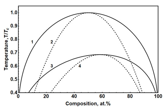
Figure 1.
Phase diagram for binary solution (1, 2) and binary solution with respect to electronic subsystem in approximation of ambipolar diffusion (3, 4). Curves 1 and 3 show the temperature dependence of equilibrium composition. The dashed lines 2 and 4 show the metastability limit.
Thus, we conclude that Cahn–Hilliard equation with variable mobility (3) can be applied for systems consisting of cations and anions in ambipolar diffusion approximation.
Different specific mechanisms can lead to anomalous diffusion processes [5,6]. The features of anomalous diffusion are often described within the continuous time random walk (CTRW) model. The decoupled version of CTRW model implies that different jump lengths and waiting (trapping) times between two successive jumps are independent random variables. Fractional-order diffusion equation can be obtained as the asymptotic equation of CTRW with power law distributions of random trapping times : (). Considering CTRW with space dependent jump probabilities, Barkai et al. [38] derived a time-fractional Fokker–Planck equation (FFPE) for the case, when the mean waiting time diverges. FFPE describes anomalous diffusion in an external force field, it is derived in the following form [39,40]:
where is particle concentration, is an external potential, K is a generalized diffusion coefficient and is the thermal energy.
Here,
is the Riemann–Liouville derivative of fractional order [15]. Fundamental solutions to Equation (5) can be found in [39,40].
The fractional diffusion equation for the simplest case has the following form:
The Fourier transform of Equation (6) leads to the expression
The flux density for diffusion described by (6) takes the form
The subdiffusive generalization of Warburg’s impedance for a semi-infinite medium can be written in the form [30]
Here, B is a frequency-independent parameter.
Based on fractional Equations (5) and (6), different generalizations of diffusion impedances can be obtained for different geometries and boundary conditions (see in [30,41,42,43,44] and references therein). In recent paper [45], effects produced by ion subdiffusion in lithium-ion cell are described within the fractional-order generalization of the single-particle model.
The similar derivation can be applied to subdiffusive Cahn–Hilliard equation with time-fractional derivatives. The subdiffusion of cations is characterized by fractional order ,
and transport of anions is characterized by fractional order
Here,
is the fractional Caputo derivative.
Eliminating the electric field from the considered system of equations, we arrive at an equation with a combination of fractional derivatives:
Denote the time-operator in the left-hand side by , and rewrite the equation in the compact form:
4. Mono-Fractional Phase-Field Subdiffusion
In the present work, we consider the role of anomalous phase field diffusion on impedance of phase transition material. In application, we limit ourselves to the case . With the latter equation can be rewritten in the form
This phase-field diffusion equation is related to the following continuity equation and generalized Fick law:
Monofractional Equation (11) can also be used to describe transport of intercalant atoms in solid particles. For example, when lithium is intercalated into some materials (LiFePO or LiMnO), the separation of the lithiated and non-lithiated phases can take place. In [11], real-time tracking of lithium transport and conversion in FeF2 nanoparticles by nanoscale imaging reveals a surprisingly fast conversion process in individual particles, with a morphological evolution resembling spinodal decomposition. The description of spinodal decomposition is usually based on the Cahn–Hilliard equation [13].
Following Bisquert and Compte [46], we also consider another type of the continuity equation
With ordinary relation for current , this system of equations leads to the following time-fractional generalization of the CH-equation:
For this case, the number of diffusing particles is not conserved. For the one-dimensional case, the diffusion equation
has clear interpretation [29,30]. In the multiple trapping model, this equation describes evolution of delocalized carriers concentration. In [46], the case (14) is classified as ‘anomalous diffusion Ia’ (AD-Ia), while case (6) is denoted as ‘anomalous diffusion Ib’.
In the following section, we apply linearization procedure to derive the response to a constant input signal with small harmonic perturbation component.
5. Impedance of Fractional Phase-Field Diffusion
Let us consider definition of impedance in electrode where conduction is related to mobility of ions in ambipolar diffusion approximation. The problem is analogous to calculation of diffusion impedance performed by Warburg. In this study, we employ CH Equation (3) with effective mixing energy (4) that describes charge transport in ambipolar diffusion approximation. The CH equation is widely used for the analysis of first-order phase transitions in solid solutions [47]. The CH Equation (3) can be easily linearized, if we apply the linear expansion of nonlinear term
where is the average concentration of ions, is the small perturbation of ions’ concentration provided by the applied periodic voltage . Leaving terms of the first order, we derive the fractional Cahn–Hilliard equation in the linearized form
Here, we introduce dimensionless variables and coefficients:
The CH equation can describe formation of phases by mechanisms of spinodal decomposition or nucleation [37]. Therefore, we assume that has the value not far from the equilibrium concentration in area of stable and metastable states. Furthermore, the restriction defines the sign of that has positive values (). Then, we apply to electrode edge () periodic potential . The potential at another edge of electrode () is supposed to be zero . We can expect that chemical potential and concentration of cations changes with the same frequency: , .
Constants , , and are determined from the boundary conditions for a particular problem.
The applied potential difference determines the carrier concentration at one edge of the cell in which phase diffusion occurs. On the other side, carriers can be locked or ejected. These boundary conditions are commonly referred to as reflective and absorbing, respectively [30]. Following the work in [48], we consider the impedance of 1D system, with reflective boundary condition, and absorbing condition, but for subdiffusive Cahn–Hilliard equation with time-fractional derivatives. One of the boundary conditions usually includes the current. This current is related to the ion concentrations through non-Fickian law in the case of anomalous phase-field diffusion. As it follows from Equation (17), the Fourier image of current is determined by the following relation:
The impedance function is determined by the following expression [42]:
Impedance response is calculated here under the following initial conditions
and the following boundary conditions. For the reflecting electrode, the boundary conditions are as follows:
while for the absorbing electrode, we have
As mentioned above, these boundary conditions are typical when considering diffusion impedance. In the case of phase diffusion, they are more variable for interpretation. In particular, consider the reflecting boundary condition. One of interpretations implies charge injection from the left flat electrode at point L, phase diffusion of ions in the region with a blocking electrode at point 0. Another interpretation is based on the method of images, which is applicable since the considered equation is linearized, spatially symmetric and local. Diffusion area can be extended to and the boundary condition at zero can be replaced by the following condition at point .
These boundary conditions correspond to the problem of intercalation/deintercalation of intercalant particles (e.g., lithium and sodium) into electrode particle specified by interval . The Cahn–Hilliard equation in this case describes phase-field diffusion of intercalated phase.
The generalized impedances take the form similar to those presented in [48], but the presence of accounts for bipolar phase field subdiffusion. For the reflecting boundary condition, we obtain the following expressions for constants in solution (18),
Details of derivation for the integer-order case are provided in Appendix of work [48]. In the time-fractional case, the derivation looks very similar. For the reflecting case, we obtain
Here,
For the absorbing case, we have
Setting , we arrive at the impedance of a semi-infinite medium:
Figure 2 shows Nyquist plots corresponding to the fractional () phase-field subdiffusion for different values of (a) and (b). The slope of the lines is determined not only by fractional exponent , but also by parameter . Warburg impedance is reproduced for and .
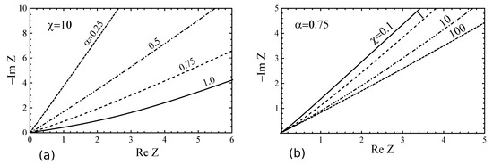
Figure 2.
Nyquist plots corresponding to the fractional () phase-field subdiffusion for different values of (a) and (b).
Figure 3 demonstrates the Nyquist plots for different boundary conditions. The case and is considered. There are different cases (a–d) for various values of and with reflecting opposite electrode. The role of phase field behavior is enhanced for larger values of . When , we arrive at ordinary diffusive () or subdiffusive () impedance responses. Subdiffusion parameter influences the shapes of arcs and slope of low-voltage tail. The phase-field character of diffusion (with increasing ) makes the transitions between the regions more abrupt.
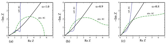
Figure 3.
Nyquist plots corresponding to the phase-field subdiffusion (, ) for different values of with reflecting boundary condition, : (a) , (b) , (c) .
The classical finite-length Warburg impedances take place at and . For normal diffusion, . If , for the reflecting and absorbing cases, we have
with
In other words, we arrive at the finite-length impedance for bipolar subdiffusion.
In case of monopolar subdiffusion , we arrive at the impedance obtained by Bisquert and Compte [46] for subdiffusion,
where is a constant dependent on l and subdiffusion coefficient.
Thus, phase-field analogs of anomalous diffusion models AD-Ib and AD-Ia considered by Bisquert and Compte [46] can be described by the following equations:
We denote these fractional generalizations of the Cahn–Hilliard (CH) equation as C-CH and RL-CH, respectively, where the first letter denotes the type of fractional time derivative used in the model (Caputo or Riemann–Liouville). The corresponding impedances can be written in the following form:
with
and functions to be specified for certain type of boundary condition. For reflecting boundary, we take
and for absorbing boundary, it is
Nyquist plots for are shown in Figure 2 and Figure 3 and described above. Nyquist plots corresponding to the RL-CH model with reflecting boundary condition for different values of and are shown in Figure 4. The slope of the low-frequency part of the Nyquist diagram is determined not only by the subdiffusion exponent, but also by the parameter.
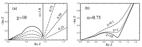
Figure 4.
Nyquist plots corresponding to the RL-CH model for different values of (a) and (b) with reflecting boundary condition ().
6. Application to Pseudo-Capacitors with Polyaniline/Carbon Nanotube Composite Electrodes
In this section, we consider an example of application of the developed model to description of impedance spectra for electrochemical supercapacitors (ESCs) with polyaniline/carbon nanotube composite electrodes. ESCs are high-capacity energy storage devices for applications requiring high power density. They are distinguished by charge storage mechanism: (1) electric double-layer (EDL) supercapacitors, where the capacitance arises due to the accumulation of charges on the electrode-electrolyte interface; (2) pseudo-capacitors with fast reversible Faraday redox reactions at the electrodes; and (3) hybrid supercapacitors that use EDL and Faraday capacitive mechanisms. To increase the active area in supercapacitors, electrodes with a highly developed surface are used. These electrodes can include porous materials based on activated carbon, carbon nanotubes, graphene oxide, foamed metals or conducting polymers and other materials.
In [44], we studied the behavior of planar microsupercapacitors (PMSC) with electrodes of MWCNT array under sinusoidal excitation, step voltage input and linear voltage input. The fractional differential model for planar supercapacitor proposed in [44] successfully describes the measured impedance spectra. Charge storage mechanism in PMSC implies the EDL formation, and the model used in [44] is based on the linear fractional diffusion equation. Here, we apply fractional phase-field diffusion model to pseudo-capacitors with PANI/MWCNT electrodes.
Polyaniline (PANI) was one of the first electroactive materials that opened the way to the fundamental and practical development of pseudo-capacitors [49]. In recent times, PANI has attracted additional attention due to its invaluable advantages in composition with other electroactive nanomaterials [50]. Short description of the system considered in our work is given in [51].
Electrodes of the pseudo-capacitor studied in this work contain vertically aligned MWCNT array (see Figure 5 and Figure 6a). The organic compound was grown by the pyrolysis method. The area of the plates is of 0.5 cm. The MWCNT layer was covered with a thin layer of polyaniline (emeraldine form), obtained by the chemical method of oxidation of an aniline solution. The thickness of PANI layer is ~250 nm. A solution of polyvinyl alcohol (PVA) and phosphoric acid was used as a layer between the plates. A schematic representation of the structure is presented in Figure 6a. The parameters of the studied system were estimated by cyclic voltammetry and impedance spectroscopy. The measurements were made with the potentiostat-galvanostat P-40X (Electrochemical Instruments). Voltammograms are measured in the range from V to V at a potential sweep speed of 20 and 100 mV/s. Impedance spectra were taken in the frequency range from 0.1 Hz to 50 kHz with an amplitude of 50 mV.
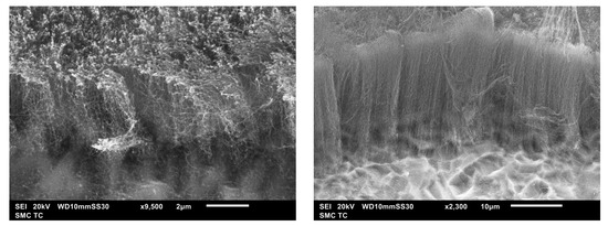
Figure 5.
SEM image of a grown MWCNT array on a titanium plate used by us for preparation of PANI-MWCNT pseudo-capacitor.
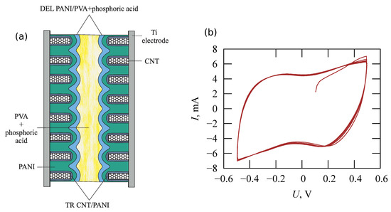
Figure 6.
Schematic representation of the cell with polyaniline/vertically aligned carbon nanotube array electrodes (a,b). Voltammogram for pseudocapacitors for potential sweep speed of 100 mV/s.
Typical voltammogram for the studied pseudo-capacitor is demonstrated in Figure 6b. The capacity determined from voltammogram is of F.
We fit measured frequency dependencies of the PANI-MWCNT pseudo-capacitor impedance by a simple equivalent circuit containing elements and defined by (22). Reasonable goodness of fit has been achieved for the simple model presented in Figure 7. Fitted parameters are following: , , , F, Ohm and Ohm·Hz, m. Changing by makes matching difficult and requires significant complication of the equivalent circuit and supplementing the model by additional elements. Comparison of measured and fitted spectra is demonstrated in Figure 8.
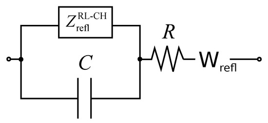
Figure 7.
Equivalent circuit model of PANI-MWCNT pseudo-capacitor. Element is described by impedance from (22) for the case of the RL-CH model with reflecting boundary condition.
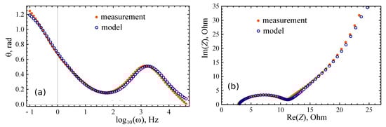
Figure 8.
Nyquist (a) and Bode (b) plots of measured and modeled impedance spectra for PANI-MWCNT pseudo-capacitor at room temperature.
The used equivalent circuit can be reasonably interpreted. In the configuration of the supercapacitor shown in Figure 6a, the transport can be modeled by a one-dimensional transfer model. The capacity of EDL formed around the MWCNTs is modeled by ideal capacitor. The open Warburg impedance describes diffusion in the interelectrode space. The series resistor takes into account the resistance in the tubes, polymer and electrolyte. Element describes phase-field ion diffusion in PANI filling the MWCNT array with reflecting boundary condition at the base of nanotube array. The RL-CH model implies non-conserving ion density that can be related to the EDL formation by fraction of ions during phase diffusion inside the MWCNT array.
The spectra modeled by circuit presented in Figure 7 for listed parameters are sensitive to impact of phase-field diffusion, that is confirmed by variation of Bode plots for different values of (Figure 9). For chosen parameters, for small values, the peak in frequency dependence of the phase shift disappears, and the height of this peak can indicate the impact of phase-field transport. However, the latter statement requires verification and separate study under different conditions and for a larger number of systems.
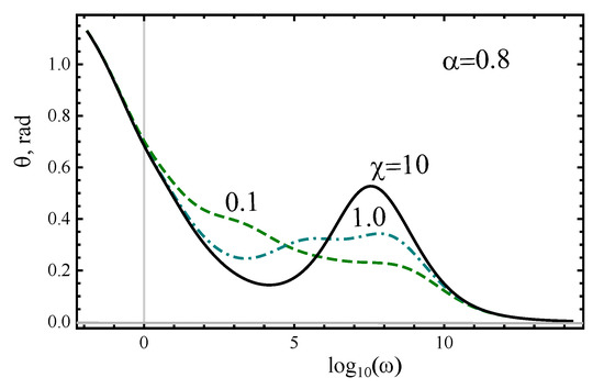
Figure 9.
Bode plots for the equivalent circuit with for different values of .
7. Conclusions
In the present work, within the framework of the phase field approach based on the fractional Cahn–Hilliard equation, the model of diffusion formation of the electric double layer is revised and the frequency dependences of the generalized Warburg impedance are derived for the case of ion transport controlled by the subdiffusion Cahn–Hilliard equation with fractional derivatives. We studied charge transfer in an electrode, where conductivity is provided by monopolar or bipolar ionic charge transfer. The driving force is the chemical potential of ions, which is described in terms of the phase field, that allows us to avoid additional calculation of the activity coefficient. We apply linearization procedure to derive the response to a constant input signal with small harmonic perturbation component, and nonlinear fractional Cahn–Hilliard equation becomes linear. Then, we solve it by means of the integral transformation method. Impedance responses for a semi-infinite medium, and for finite-length cell with reflecting and absorbing boundary conditions for time-fractional Cahn–Hilliard equation are calculated and described.
The model is applied to description of impedance spectra of pseudo-capacitors with polyaniline/carbon nanotube composite electrodes. We fitted measured frequency dependencies of the PANI-MWCNT pseudo-capacitor impedance by a simple equivalent circuit containing elements and defined by (22). Reasonable goodness of fit has been achieved for the simple model presented in Figure 7, that can be provided by clear interpretation. The configuration of our pseudo-capacitor implies one-dimensional transfer model. The capacity of EDL formed around MWCNTs is modeled by ideal capacitor. The open Warburg impedance describes diffusion in interelectrode space. The series resistor takes into account the resistance in the tubes, polymer and electrolyte. Element describes phase-field ion diffusion in PANI filling the MWCNT array with reflecting boundary condition at the base of nanotube array. The RL-CH model implies non-conserving ion density that can be related to the EDL formation by fraction of ions during phase diffusion inside the MWCNT array. Changing of by makes matching difficult and requires significant complication of the equivalent circuit and supplementing the model by additional elements. We show that the assumption of phase-field diffusion plays an important role in this approximation. The peak in frequency dependence of phase is sensitive to the -value and can indicate the impact of phase-field diffusion.
Author Contributions
Conceptualization, R.T.S. and P.E.L.; methodology, R.T.S. and P.E.L.; validation, I.O.Y. and E.P.K.; investigation, R.T.S. and P.E.L.; resources, I.O.Y. and E.P.K.; data curation, E.P.K.; writing—original draft preparation, R.T.S. and P.E.L.; writing—review and editing, R.T.S. and P.E.L.; visualization, I.O.Y. and E.P.K.; project administration, R.T.S. and E.P.K.; funding acquisition, R.T.S. and E.P.K. All authors have read and agreed to the published version of the manuscript.
Funding
P.E.L., R.T.S. and I.O.Y. acknowledge the support from the Russian Science Foundation (project No. 19-71-10063), and E.P.K. acknowledges the support from the Ministry of Science and Higher Education of the Russian Federation (project No. 0591-2021-0002) and the Russian Federation President program (grant MK-1823.2021.4).
Institutional Review Board Statement
Not applicable.
Informed Consent Statement
Not applicable.
Data Availability Statement
Not applicable.
Conflicts of Interest
The authors declare no conflict of interest.
References
- Barsoukov, E.; Macdonald, J.R. Impedance Spectroscopy Theory, Experiment, and Applications, 2nd ed.; John Wiley & Sons, Inc.: Hoboken, NJ, USA, 2005. [Google Scholar]
- Orazem, M.E.; Tribollet, B. Electrochemical Impedance Spectroscopy; John Wiley & Sons, Inc.: Hoboken, NJ, USA, 2008; pp. 383–389. [Google Scholar]
- Taylor, S.R.; Gileadi, E. Physical interpretation of the Warburg impedance. Corrosion 1995, 51, 664–671. [Google Scholar] [CrossRef]
- Huang, J. Diffusion impedance of electroactive materials, electrolytic solutions and porous electrodes: Warburg impedance and beyond. Electrochim. Acta 2018, 281, 170–188. [Google Scholar] [CrossRef]
- Metzler, R.; Klafter, J. The random walk’s guide to anomalous diffusion: A fractional dynamics approach. Phys. Rep. 2000, 339, 1–77. [Google Scholar] [CrossRef]
- Uchaikin, V.V.; Sibatov, R. Fractional Kinetics in Solids: Anomalous Charge Transport in Semiconductors, Dielectrics, and Nanosystems; World Scientific: Singapore, 2013. [Google Scholar]
- Guyer, J.E.; Boettinger, W.J.; Warren, J.A.; McFadden, G.B. Phase field modeling of electrochemistry. I. Equilibrium. Phys. Rev. E 2004, 69, 021603. [Google Scholar] [CrossRef] [PubMed] [Green Version]
- Guyer, J.E.; Boettinger, W.J.; Warren, J.A.; McFadden, G.B. Phase field modeling of electrochemistry. II. Kinetics. Phys. Rev. E 2004, 69, 021604. [Google Scholar] [CrossRef] [PubMed] [Green Version]
- Ferguson, T.R.; Bazant, M.Z. Nonequilibrium thermodynamics of porous electrodes. J. Electrochem. Soc. 2012, 159, A1967. [Google Scholar] [CrossRef]
- Fleck, M.; Federmann, H.; Pogorelov, E. Phase-field modeling of Li-insertion kinetics in single LiFePO4-nano-particles for rechargeable Li-ion battery application. Comput. Mater. Sci. 2018, 153, 288–296. [Google Scholar] [CrossRef] [Green Version]
- Wang, F.; Yu, H.C.; Chen, M.H.; Wu, L.; Pereira, N.; Thornton, K.; Van der Ven, A.; Zhu, Y.; Amatucci, G.G.; Graetz, J. Tracking lithium transport and electrochemical reactions in nanoparticles. Nat. Commun. 2012, 3, 1201. [Google Scholar] [CrossRef] [PubMed] [Green Version]
- Cahn, J.W.; Hilliard, J.E. Free energy of a nonuniform system. I. Interfacial free energy. J. Chem. Phys. 1958, 28, 258–267. [Google Scholar] [CrossRef]
- Cahn, J.W. On spinodal decomposition. Acta Metall. 1961, 9, 795–801. [Google Scholar] [CrossRef]
- Chen, C.; Ciucci, F. Generalized transport model for phase transition with memory. Phys. Lett. A 2013, 377, 2668–2672. [Google Scholar] [CrossRef]
- Samko, S.G.; Kilbas, A.A.; Marichev, O.I. Integrals and Derivatives of Fractional Order and Some of Their Applications; Nauka i Tekhnika: Minsk, Belarus, 1987. (In Russian) [Google Scholar]
- Zaslavsky, G.M. Chaos, fractional kinetics, and anomalous transport. Phys. Rep. 2002, 371, 461–580. [Google Scholar] [CrossRef]
- Schneider, W.R.; Wyss, W. Fractional diffusion and wave equations. J. Math. Phys. 1989, 30, 134–144. [Google Scholar] [CrossRef]
- Mainardi, F. Fractional relaxation-oscillation and fractional diffusion-wave phenomena. Chaos Solitons Fractals 1996, 7, 1461–1477. [Google Scholar] [CrossRef]
- Hilfer, R. Fractional diffusion based on Riemann-Liouville fractional derivatives. J. Phys. Chem. B 2000, 104, 3914–3917. [Google Scholar] [CrossRef] [Green Version]
- Uchaikin, V.V.; Sibatov, R.T. Fractional differential kinetics of dispersive transport as the consequence of its self-similarity. JETP Lett. 2007, 86, 512–516. [Google Scholar] [CrossRef]
- Uchaikin, V.V.; Ambrozevich, A.S.; Sibatov, R.T.; Ambrozevich, S.A.; Morozova, E.V. Memory and nonlinear transport effects in charging-discharging of a supercapacitor. Tech. Phys. 2016, 61, 250–259. [Google Scholar] [CrossRef]
- Akagi, G.; Schimperna, G.; Segatti, A. Fractional Cahn–Hilliard, Allen–Cahn and porous medium equations. J. Differ. Equ. 2016, 261, 2935–2985. [Google Scholar] [CrossRef] [Green Version]
- Liu, H.; Cheng, A.; Wang, H.; Zhao, J. Time-fractional Allen–Cahn and Cahn–Hilliard phase-field models and their numerical investigation. Comput. Math. Appl. 2018, 76, 1876–1892. [Google Scholar] [CrossRef]
- Tripathi, N.K.; Das, S.; Ong, S.H.; Jafari, H.; Al Qurashi, M.M. Solution of time-fractional Cahn–Hilliard equation with reaction term using homotopy analysis method. Adv. Mech. Eng. 2017, 9, 1687814017740773. [Google Scholar] [CrossRef]
- Nigmatullin, R.R. The realization of the generalized transfer equation in a medium with fractal geometry. Phys. Status Solidi (b) 1986, 133, 425–430. [Google Scholar] [CrossRef]
- Nigmatullin, R.R. Fractional integral and its physical interpretation. Theor. Math. Phys. 1992, 90, 242–251. [Google Scholar] [CrossRef]
- Scher, H.; Montroll, E.W. Anomalous transit-time dispersion in amorphous solids. Phys. Rev. B 1975, 12, 2455. [Google Scholar] [CrossRef]
- Saichev, A.I.; Zaslavsky, G.M. Fractional kinetic equations: Solutions and applications. Chaos Interdiscip. J. Nonlinear Sci. 1997, 7, 753–764. [Google Scholar] [CrossRef] [PubMed] [Green Version]
- Sibatov, R.T.; Uchaikin, V.V. Fractional differential kinetics of charge transport in unordered semiconductors. Semiconductors 2007, 41, 335–340. [Google Scholar] [CrossRef]
- Bisquert, J. Fractional diffusion in the multiple-trapping regime and revision of the equivalence with the continuous-time random walk. Phys. Rev. Lett. 2003, 91, 010602. [Google Scholar] [CrossRef] [PubMed] [Green Version]
- Sibatov, R.; Shulezhko, V.; Svetukhin, V. Fractional derivative phenomenology of percolative phonon-assisted hopping in two-dimensional disordered systems. Entropy 2017, 19, 463. [Google Scholar] [CrossRef]
- Ainsworth, M.; Mao, Z. Analysis and approximation of a fractional Cahn–Hilliard equation. SIAM J. Numer. Anal. 2017, 55, 1689–1718. [Google Scholar] [CrossRef] [Green Version]
- Weng, Z.; Zhai, S.; Feng, X. A Fourier spectral method for fractional-in-space Cahn–Hilliard equation. Appl. Math. Model. 2017, 42, 462–477. [Google Scholar] [CrossRef]
- Caputo, M.; Fabrizio, M. Damage and fatigue described by a fractional derivative model. J. Comput. Phys. 2015, 293, 400–408. [Google Scholar] [CrossRef]
- Xia, H.; Tang, G.; Ma, J.; Hao, D.; Xun, Z. Scaling behaviour of the time-fractional Kardar-Parisi-Zhang equation. J. Phys. Math. Theor. 2011, 44, 275003. [Google Scholar] [CrossRef]
- L’vov, P.E.; Svetukhin, V.V. Simulation of the first order phase transitions in binary alloys with variable mobility. Model. Simul. Mater. Sci. Eng. 2017, 25, 075006. [Google Scholar] [CrossRef]
- Provatas, N.; Elder, K. Phase-Field Methods in Materials Science and Engineering; John Wiley & Sons: Hoboken, NJ, USA, 2011. [Google Scholar]
- Barkai, E.; Metzler, R.; Klafter, J. From continuous time random walks to the fractional Fokker–Planck equation. Phys. Rev. E 2000, 61, 132. [Google Scholar] [CrossRef] [PubMed]
- Barkai, E. Fractional Fokker-Planck equation, solution, and application. Phys. Rev. E 2001, 63, 046118. [Google Scholar] [CrossRef] [PubMed] [Green Version]
- Metzler, R.; Barkai, E.; Klafter, J. Anomalous diffusion and relaxation close to thermal equilibrium: A fractional Fokker-Planck equation approach. Phys. Rev. Lett. 1999, 82, 3563. [Google Scholar] [CrossRef] [Green Version]
- Macdonald, J.R.; Evangelista, L.R.; Lenzi, E.K.; Barbero, G. Comparison of impedance spectroscopy expressions and responses of alternate anomalous Poisson? Nernst? Planck diffusion equations for finite-length situations. J. Phys. Chem. C 2011, 115, 7648–7655. [Google Scholar] [CrossRef]
- Ciuchi, F.; Mazzulla, A.; Scaramuzza, N.; Lenzi, E.K.; Evangelista, L.R. Fractional diffusion equation and the electrical impedance: Experimental evidence in liquid-crystalline cells. J. Phys. Chem. C 2012, 116, 8773–8777. [Google Scholar] [CrossRef]
- Sibatov, R.T.; Uchaikin, V.V. Fractional kinetics of charge carriers in supercapacitors. In Volume 8 Applications in Engineering, Life and Social Sciences, Part B; De Gruyter: Berlin, Germany, 2019; pp. 87–118. [Google Scholar]
- Kitsyuk, E.P.; Sibatov, R.T.; Svetukhin, V.V. Memory effect and fractional differential dynamics in planar microsupercapacitors based on multiwalled carbon nanotube arrays. Energies 2020, 13, 213. [Google Scholar] [CrossRef] [Green Version]
- Sibatov, R.T.; Svetukhin, V.V.; Kitsyuk, E.P.; Pavlov, A.A. Fractional differential generalization of the single particle model of a lithium-ion cell. Electronics 2019, 8, 650. [Google Scholar] [CrossRef] [Green Version]
- Bisquert, J.; Compte, A. Theory of the electrochemical impedance of anomalous diffusion. J. Electroanal. Chem. 2001, 499, 112–120. [Google Scholar] [CrossRef]
- Pego, R.L. Front migration in the nonlinear Cahn-Hilliard equation. Proc. R. Soc. Lond. A Math. Phys. Sci. 1989, 422, 261–278. [Google Scholar]
- Ciucci, F.; Lai, W. Electrochemical impedance spectroscopy of phase transition materials. Electrochim. Acta 2012, 81, 205–216. [Google Scholar] [CrossRef]
- Eftekhari, A.; Li, L.; Yang, Y. Polyaniline supercapacitors. J. Power Sources 2017, 347, 86–107. [Google Scholar] [CrossRef]
- Gupta, V.; Miura, N. Polyaniline/single-wall carbon nanotube (PANI/SWCNT) composites for high performance supercapacitors. Electrochim. Acta 2006, 52, 1721–1726. [Google Scholar] [CrossRef]
- Yavtushenko, I.O.; Sibatov, R.T.; Somov, A.I.; Makhmud-Akhunov, M.Y. Fractional circuit model for supercapacitors with polyaniline/carbon nanotube composite-based electrodes. J. Phys. Conf. Ser. 2020, 1695, 012039. [Google Scholar] [CrossRef]
Publisher’s Note: MDPI stays neutral with regard to jurisdictional claims in published maps and institutional affiliations. |
© 2021 by the authors. Licensee MDPI, Basel, Switzerland. This article is an open access article distributed under the terms and conditions of the Creative Commons Attribution (CC BY) license (https://creativecommons.org/licenses/by/4.0/).