Parametric Family of Root-Finding Iterative Methods: Fractals of the Basins of Attraction

Abstract

Research interest in iterative multipoint schemes to solve nonlinear problems has increased recently because of the drawbacks of point-to-point methods, which need high-order derivatives to increase the order of convergence. However, this order is not the only key element to classify the iterative schemes. We aim to design new multipoint fixed point classes without memory, that improve or bring together the existing ones in different areas such as computational efficiency, stability and also convergence order. In this manuscript, we present a family of parametric iterative methods, whose order of convergence is four, that has been designed by using composition and weight function techniques. A qualitative analysis is made, based on complex discrete dynamics, to select those elements of the class with best stability properties on low-degree polynomials. This stable behavior is directly related with the simplicity of the fractals defined by the basins of attraction. In the opposite, particular methods with unstable performance present high-complexity in the fractals of their basins. The stable members are demonstrated also be the best ones in terms of numerical performance of non-polynomial functions, with special emphasis on Colebrook-White equation, with wide applications in Engineering.

1. Introduction

The solution of nonlinear equations is a typical problem in engineering and experimental sciences. Problems with gases, liquids, and mechanics require calculating the roots of the equations with the iterative. Among Chemistry problems needing to solve this kind of equations are chemical equilibrium problems, global reaction rates in packed bed reactors [1], radioactive transfer [2], continuous stirred tank reactors (see [3]) or to simulate flow transport in a pipe [4]. In general, these equations cannot be solved analytically and we must resort to iterative methods to approximate their solutions. With the increasing speed of computers, numerical techniques have become indispensable for scientists and engineers. The principle of these methods is to approach the solution $x^{*}$ of a nonlinear equation of the form $f\left(x\right)=0$, through a sequence of iterations, starting from an initial estimation of $x_0$. The most known and widely used method to solve nonlinear equations is Newton’s scheme, whose iterative expression is

$$x_{k+1}=x_k-{\displaystyle \frac{f\left(x_k\right)}{f^{\prime }\left(x_k\right)}},k=0,1,2,\dots$$

(1)

and it presents the quadratic convergence. This method requires two functional evaluations $(d=2)$, one of the function and one of its first derivative, per iteration. Kung-Traub’s conjecture [5] states that an iterative method without memory for finding a simple zero of an scalar equation is optimal if its order of convergence is equal to $2^{d-1}$. Therefore, Newton’s method is optimal.

Many variants of Newton’s scheme have been constructed by means of several techniques, setting different multistep schemes. Some of them use Adomian decomposition (see [6], for instance). Another kind of iterative schemes are those of using higher-order derivatives, for example in Chebyshev-type methods by some approximation [7]. Moreover, the direct composition of known methods with a later treatment to reduce the number of functional evaluations is often used in order to generate new methods. Indeed, a weight-function procedure has been used recently to increase the convergence order of known methods [8,9], in order to obtain optimal schemes.

Moreover, it is known that the sensitiveness of a scheme to the initial seeds increases as well as does the order [10]. It is widely accepted that the dynamical behavior of the rational function related to an iterative scheme provides us with important information about its stability and reliability [11]. In these terms, Amat et al. in [12] described the dynamical performance of some known families of iterative methods. More recently, in [9,13,14,15,16,17], different authors analyze the qualitative behavior of several known methods or classes of iterative schemes. Most of these studies demonstrate some elements with very stable behavior, which is proven to be useful in practice, and also different pathological performances, such as attracting fixed points different from the solution of the problem, periodic orbits, etc. The key tool to understanding the behavior of the different members of the family are the parameter planes.

We aim to design a new multipoint fixed point class, without memory, that improves or brings together the existing ones, as for example appears in [18,19], in different areas such as computational efficiency, stability and convergence order. There exists a wide number of optimal iterative methods with different orders of convergence, such as [15]; some of them can be grouped as special cases of our proposed class of iterative procedures.

Let us search the conditions that parameter $\gamma$ and G function, from the iterative expression

$$y_k=x_k-\gamma {\displaystyle \frac{f\left(x_k\right)}{f^{\prime }\left(x_k\right)}},$$

$$x_{k+1}=x_k-G\left({\eta }_k\right){\displaystyle \frac{f\left(x_k\right)}{f^{\prime }\left(x_k\right)}},k=0,1,2,\dots ,$$

(2)

must meet to reach the fourth convergence order, where the variable of the weight function is ${\eta }_k={\displaystyle \frac{f^{\prime }\left(y_k\right)}{f^{\prime }\left(x_k\right)}}$.

The rest of the paper is organized as follows: in Section 2, we prove the fourth-order convergence of the proposed class of iterative methods, under some conditions. Moreover, a particular subclass is presented and some known methods have been found as special cases of our proposed family. Section 3 is devoted to the qualitative study of our proposed parametric class of iterative schemes, giving rise to some stable and unstable members, that are numerically checked in Section 4, along with other known methods. These numerical tests demonstrate the good performance in both academical and applied problems, such as the Colebrook-White equation.

2. Convergence Analysis

In the next result, we present the sufficient conditions of the weight function G and parameter $\gamma$ that guarantee the convergence of the proposed class.

Theorem 1.

Let$f:I\subseteq \mathbb{R}\to \mathbb{R}$be a sufficiently differentiable function in an open interval I and$x^{*}\in I$a simple root of equation$f\left(x\right)=0$. Let$G\left(\eta \right)$be a real function satisfying$|G^{‴}\left(1\right)|<+\infty$, $G^{″}\left(1\right)={\displaystyle \frac{9}{4}}$, $G^{\prime }\left(1\right)=-{\displaystyle \frac{3}{4}}$and$G\left(1\right)=1$. If$\gamma ={\displaystyle \frac{2}{3}}$and we choose an initial approximation$x_0$close enough to$x^{*}$, then the family of iterative methods defined by

$$y_k=x_k-\gamma {\displaystyle \frac{f\left(x_k\right)}{f^{\prime }\left(x_k\right)}},$$

$$x_{k+1}=x_k-G\left(\eta \right){\displaystyle \frac{f\left(x_k\right)}{f^{\prime }\left(x_k\right)}},k=0,1,2,\dots ,$$

(3)

satisfies the error equation below:

$$e_{k+1}=\left[\left(5+{\displaystyle \frac{32G^{‴}\left(1\right)}{81}}\right)c_2^3-c_2{c}_3+{\displaystyle \frac{c_4}{9}}\right]e_k^4+O\left(e_k^5\right),$$

where$c_k={\displaystyle \frac{1}{k!}}{\displaystyle \frac{f^{\left(k\right)}\left(x^{*}\right)}{f^{\prime }\left(x^{*}\right)}}$, $k=2,3,\dots$, ${\eta }_k={\displaystyle \frac{f^{\prime }\left(y_k\right)}{f^{\prime }\left(x_k\right)}}$and$e_k=x_k-x^{*}$, $k=1,2,\dots$. Therefore, all the members of class (3) converges to $x^{*}$ with an order of convergence four.

Proof. 

Let $x^{*}$ be a simple zero of f. As f is a sufficiently differentiable function, using the Taylor expansion for $f\left(x_k\right)$ and $f^{\prime }\left(x_k\right)$ at about $x^{*}$, we obtain

$$\begin{array}{ccc}\hfill f\left(x_k\right)& =& f^{\prime }\left(x^{*}\right)[e_k+c_2{e}_k^2+c_3{e}_k^3+c_4{e}_k^4]+\mathcal{O}\left(e_k^5\right),\hfill \end{array}$$

and

$$\begin{array}{ccc}\hfill f^{\prime }\left(x_k\right)& =& f^{\prime }\left(x^{*}\right)[1+2c_2{e}_k+3c_3{e}_k^2+4c_4{e}_k^3]+\mathcal{O}\left(e_k^4\right).\hfill \end{array}$$

From these expressions, we obtain the first step

$$\begin{array}{ccc}\hfill y_k& =& (1-\gamma )e_k+\gamma c_2{e}_k^2-2\left(\gamma (c_2^2-c_3)\right)e_k^3+\gamma (4c_2^3-7c_2{c}_3+3c_4)e_k^4+\mathcal{O}\left(e_k^5\right).\hfill \end{array}$$

Expanding in Taylor’s series $f\left(y_k\right)$, around $x^{*}$,

$$\begin{array}{ccc}\hfill f^{\prime }\left(y_k\right)& =& f^{\prime }\left(x^{*}\right)\left[1-2\left((-1+\gamma )c_2\right)e_k+(2\gamma c_2^2+3{(-1+\gamma )}^2{c}_3)e_k^2+2(-2\gamma c_2^3+(5-3\gamma )\gamma c_2{c}_3-2{(-1+\gamma )}^3{c}_4)e_k^3\right]+\mathcal{O}\left(e_k^4\right).\hfill \end{array}$$

and then, combining these expressions,

$$\begin{array}{ccc}\hfill \eta & =& 1-2\left(\gamma c_2\right)e_k+3\gamma (2c_2^2+(-2+\gamma )c_3)e_k^2-4\left(\gamma (4c_2^3+(-7+3\gamma )c_2{c}_3+(3-3\gamma +{\gamma }^2)c_4)\right)e_k^3+\mathcal{O}\left(e^4\right).\hfill \end{array}$$

(4)

Let us represent function G by its Taylor polynomial of the third order around 1, as $\eta$ tends to 1 when k tend to infinity:

$$\begin{array}{cc}\hfill G\left(\eta \right)=& G\left(1\right)-2\left(\gamma G^{\prime }\left(1\right)c_2\right)e_k+\gamma (2(3G^{\prime }\left(1\right)+\gamma G^{″}\left(1\right))c_2^2+3(-2+\gamma )G^{\prime }\left(1\right)c_3)e_k^2\hfill \\ & +({\displaystyle \frac{-4}{3}}\gamma (12G^{\prime }\left(1\right)+\gamma (9G^{″}\left(1\right)+\gamma G^{‴}\left(1\right)))c_2^3-2\gamma (2(-7+3\gamma )G^{\prime }\left(1\right)+3(-2+\gamma )\gamma G^{″}\left(1\right))c_2{c}_3\hfill \\ & -4\gamma (3-3\gamma +{\gamma }^2)G^{\prime }\left(1\right)c_4)e_k^3+\mathcal{O}\left(e_k^4\right).\hfill \end{array}$$

Therefore,

$$\begin{array}{cc}\hfill e_{k+1}=& (1-G\left(1\right))e_k+(G\left(1\right)+2\gamma G^{\prime }\left(1\right))c_2{e}_k^2+(-2(G\left(1\right)+\gamma (4G^{\prime }\left(1\right)+\gamma G^{″}\left(1\right))))c_2^2+\left((2G\left(1\right)-3(-2+\gamma )\gamma G^{\prime }\left(1\right))c_3\right)e_k^3\hfill \\ & +(\left(4G\left(1\right)+26\gamma G^{\prime }\left(1\right)+14{\gamma }^2{G}^{″}\left(1\right)+{\displaystyle \frac{4{\gamma }^3{G}^{‴}\left(1\right)}{3}}\right)c_2^3+(-7G\left(1\right)+\gamma ((-38+15\gamma )G^{\prime }\left(1\right)+6(-2+\gamma )\gamma G^{″}\left(1\right)))c_2{c}_3\hfill \\ & +(3G\left(1\right)+4a(3-3a+a^2)G^{\prime }\left(1\right))c_4)e_k^4+\mathcal{O}\left(e_k^5\right).\hfill \end{array}$$

To achieve the order of convergence four, it is necessary to force the coefficients of $e_k^p$, $p=1,2,3$ to be null. Then, we obtain that the following conditions are needed: $\gamma ={\displaystyle \frac{2}{3}}$, $G^{″}\left(1\right)={\displaystyle \frac{9}{4}}$, $G^{\prime }\left(1\right)={\displaystyle \frac{-3}{4}}$ and $G\left(1\right)=1$.

By substituting them in the error equation, we obtain that it is a function of $G^{‴}\left(1\right)$,

$$e_{k+1}=\left[\left(5+{\displaystyle \frac{32G^{‴}\left(1\right)}{81}}\right)c_2^3-c_2{c}_3+{\displaystyle \frac{c_4}{9}}\right]e_k^4+\mathcal{O}\left(e_k^5\right),$$

and $|G^{‴}\left(1\right)|<+\infty$ must be satisfied. □

Some known schemes can be found as particular cases of family (3) satisfying all the conditions of Theorem 1. Firstly, the well-known Jarratt’s method [20], with the iterative expression

$$\begin{array}{ccc}\hfill y_k& =& x_k-\frac{2}{3}{\displaystyle \frac{f\left(x_k\right)}{f^{\prime }\left(x_k\right)}},\hfill \\ \hfill x_{k+1}& =& x_k-\frac{1}{2}\frac{3f^{\prime }\left(y_k\right)+f^{\prime }\left(x_k\right)}{3f^{\prime }\left(y_k\right)-f^{\prime }\left(x_k\right)}{\displaystyle \frac{f\left(x_k\right)}{f^{\prime }\left(x_k\right)}},k=0,1,2,\dots ,\hfill \end{array}$$

where $G\left(\eta \right)={\displaystyle \frac{3\eta +1}{6\eta -2}}$.

Moreover, the method designed by Hueso et al. in [21], with iterative expression

$$\begin{array}{ccc}\hfill y_k& =& x_k-\frac{2}{3}{\displaystyle \frac{f\left(x_k\right)}{f^{\prime }\left(x_k\right)}},\hfill \\ \hfill x_{k+1}& =& x_k-\left(-\frac{1}{2}+\frac{9}{8}\frac{f^{\prime }\left(x_k\right)}{f^{\prime }\left(y_k\right)}+\frac{3}{8}\frac{f^{\prime }\left(y_k\right)}{f^{\prime }\left(x_k\right)}\right){\displaystyle \frac{f\left(x_k\right)}{f^{\prime }\left(x_k\right)}},k=0,1,2,\dots ,\hfill \end{array}$$

where $G\left(\eta \right)=-{\displaystyle \frac{1}{2}}+{\displaystyle \frac{9}{8\eta }}+{\displaystyle \frac{3}{8}}\eta$ and the scheme from Khattri and Abbasbandi constructed in [22], defined as

$$\begin{array}{ccc}\hfill y_k& =& x_k-\frac{2}{3}{\displaystyle \frac{f\left(x_k\right)}{f^{\prime }\left(x_k\right)}},\hfill \\ \hfill x_{k+1}& =& x_k-\left(1+\frac{21}{8}\frac{f^{\prime }\left(y_k\right)}{f^{\prime }\left(x_k\right)}-\frac{9}{8}{\left(\frac{f^{\prime }\left(y_k\right)}{f^{\prime }\left(x_k\right)}\right)}^2+\frac{15}{8}{\left(\frac{f^{\prime }\left(y_k\right)}{f^{\prime }\left(x_k\right)}\right)}^3\right){\displaystyle \frac{f\left(x_k\right)}{f^{\prime }\left(x_k\right)}},k=0,1,2,\dots \hfill \end{array}$$

are particular members of the most general proposed class of iterative methods (3) with $G\left(\eta \right)=1+{\displaystyle \frac{21}{8}}\eta -{\displaystyle \frac{9}{2}}{\eta }^2+{\displaystyle \frac{15}{8}}{\eta }^3$.

On the other hand, by using the conditions deduced in the previous result, we select a particular subclass of iterative methods, depending on a parameter $\alpha$, whose iterative expression is

$$y_k=x_k-{\displaystyle \frac{2}{3}}{\displaystyle \frac{f\left(x_k\right)}{f^{\prime }\left(x_k\right)}},$$

(5)

$$x_{k+1}=y_k-\left(1-{\displaystyle \frac{3}{4}}(\eta -1)+{\displaystyle \frac{9}{8}}{(\eta -1)}^2+\alpha {(\eta -1)}^3\right){\displaystyle \frac{f\left(x_k\right)}{f^{\prime }\left(x_k\right)}},k=0,1,2,\dots$$

Let us remark that all the members of this family of iterative schemes have fourth-order of convergence, as they satisfy all the hypothesis of Theorem 1. The differences in their performance can be studied by using the tools of complex discrete dynamics; so, the wideness of the sets of converging initial estimations can be deduced depending on $\alpha$.

3. Stability Analysis

In order to study the dynamical behaviour of the iterative methods described in (5), it is necessary to recall a few concepts. Let us consider a rational function $R:\widehat{\mathbb{C}}\to \widehat{\mathbb{C}}$. The successive application of the operator R on one point $z_0\in \widehat{\mathbb{C}}$ is defined as the orbit of this point [12,23]:

$$\{z_0,R\left(z_0\right),R^2\left(z_0\right),\dots ,R^n\left(z_0\right),\dots \},$$

where $R^n\left(z_0\right)$ means R applied on $z_0$, n times. In our context, R is obtained by applying the class of iterative methods on a quadratic polynomial $p\left(z\right)$.

Thus, a fixed point $z^F\in \widehat{\mathbb{C}}$ of R satisfies $R\left(z_F\right)=z_F$. It is worthy to notice that it is possible to find fixed points of R that are not roots of the polynomial; in this case, those points are called strange fixed points. The stability of fixed points is classified as follows:

• Attractive if $|R^{\prime }\left(z^F\right)| <1$.
• Parabolic or Neutral if $|R^{\prime }\left(z^F\right)| =1$.
• Repulsive if $|R^{\prime }\left(z^F\right)| >1$.
• Superattractive if $R^{\prime }\left(z^F\right)=0$.

On the other hand, the basins of attraction [24] determine the final state of the orbit of any point in the complex plane after successive application of operator R. We define the basin of attraction of a fixed point $z^F\in \widehat{\mathbb{C}}$ as the set of preimages of any order that meets it:

$$\mathcal{A}\left(z^F\right)=\{z_0\in \widehat{\mathbb{C}}:R^n\left(z_0\right)\to z^F,n\to +\infty \}.$$

Moreover, the roots of the equation $R^{\prime }\left(z_0\right)=0$ are called critical points of operator R. Their asymptotic performance plays an important role in the stability of the method [25]. Moreover, in the connected component of the basin of attraction holding the attractor, there exists one critical point. Indeed, superattracting fixed points are also critical points; furthermore, critical points not being zeros of $p\left(z\right)$ are defined as free critical points.

On the other hand, the union of the basins of attraction defines the Fatou set of R. Its complementary set in $\widehat{\mathbb{C}}$ is called the Julia set.

In this section, we analyze the dynamical behavior of fourth-order parametric family (5) on the quadratic polynomial $p\left(z\right)=(z-a)(z-b)$, where $a,b\in \mathbb{C}$. So, a rational function $O_p\left(z\right)$ is obtained, depending on the parameter of the class, $alpha$, and also depending on the roots a and b. To obtain a simpler operator, as the fixed point operator satisfies the Scaling Theorem, we use the Möbius transformation [23]

$$\begin{array}{c}\hfill M\left(z\right)=\frac{z-a}{z-b},M^{-1}\left(z\right)=\frac{zb-a}{z-1},\end{array}$$

with properties:

$$\begin{array}{c}\hfill M(\infty )=1,M\left(a\right)=0,M\left(b\right)=\infty ,\end{array}$$

that yields a rational function that, being conjugated to $O_p\left(z\right)$ (and therefore, with equivalent dynamical behavior), does no longer depend on a and b:

$$O_{\alpha }\left(z\right)=\left(M\circ O_p\circ M^{-1}\right)\left(z\right)=z^4\frac{135+64\alpha +378z+378z^2+162z^3+27z^4}{2+162z+378z^2+378z^3+135z^4+64\alpha z^4}.$$

By solving equation $O_{\alpha }\left(z\right)=z$, the fixed points of the rational function are obtained. Among them are $z=0$ and $z=\infty$, coming from the roots of the polynomial previous to the Möbius map. The asymptotic behavior of all the fixed points plays a key role in the stability of the iterative methods involved, as the convergence to fixed points different from the roots means an important drawback for an iterative method; thus, we proceed below with this analysis.

A direct result of the Möbius transformation applied on this rational function is the conjugacy by the inverse,

$$\frac{1}{O_{\alpha }\left(z\right)}=O_{\alpha }\left(\frac{1}{z}\right).$$

The immediate consequences of this result are:

(a)

If $O_{\alpha }\left(z^F\right)=z^F$, then $O_{\alpha }(1/z^F)=1/z^F$.

(b)

Except for some specific values of the $\alpha$ simplifying the operator, $z=1$ is an strange fixed point of rational operator $O_{\alpha }\left(z\right)$.

(c)

The stability function of two conjugate fixed points coincide,

$$O_{\alpha }^{\prime }\left(z^F\right)=1/O_{\alpha }^{\prime }\left(z^F\right).$$

3.1. Performance of the Strange Fixed Points

The behavior of fixed points different from $z=0$ and $z=\infty$ depends on $\alpha$. In the following result, the stability of $z=1$ is established.

Theorem 2.

$z=1$is an strange fixed point of$O_{\alpha }\left(z\right)$if$\alpha \ne -\frac{135}{8}$. Thus, $z=1$is attracting if$\left|z+\frac{135}{8}\right|>54$, parabolic or neutral when$\left|z+\frac{135}{8}\right|=54$.

Proof. 

The behavior of $z=1$ is given by

$$\left|O_{\alpha }^{\prime }\left(1\right)\right|=\left|\frac{432}{8\alpha +135}\right|.$$

Thus,

$$\left|\frac{432}{8\alpha +135}\right|\le 1 \mathrm{is} \mathrm{equivalent} \mathrm{to} 432\le \left|8\alpha +135\right|.$$

Let us denote $\alpha =a+ib$. Then,

$$168399<16(135a+4a^2+4b^2)$$

and

$$b^2+{(a+135/8)}^2>2916={54}^2.$$

Therefore,

$$\left|O_{\alpha }^{\prime }\left(1\right)\right|\le 1\mathrm{if} \mathrm{and} \mathrm{only} \mathrm{if}\left|z+\frac{135}{8}\right|>54.$$

Finally, if $\alpha$ satisfies $\left|z+\frac{135}{8}\right|<54$, then $\left|O_{\alpha }^{\prime }\left(1\right)\right|>1$ and $z=1$ is a repulsive point. It is clear that it is parabolic in the boundary $\left|O_{\alpha }^{\prime }\left(1\right)\right|=1$. □

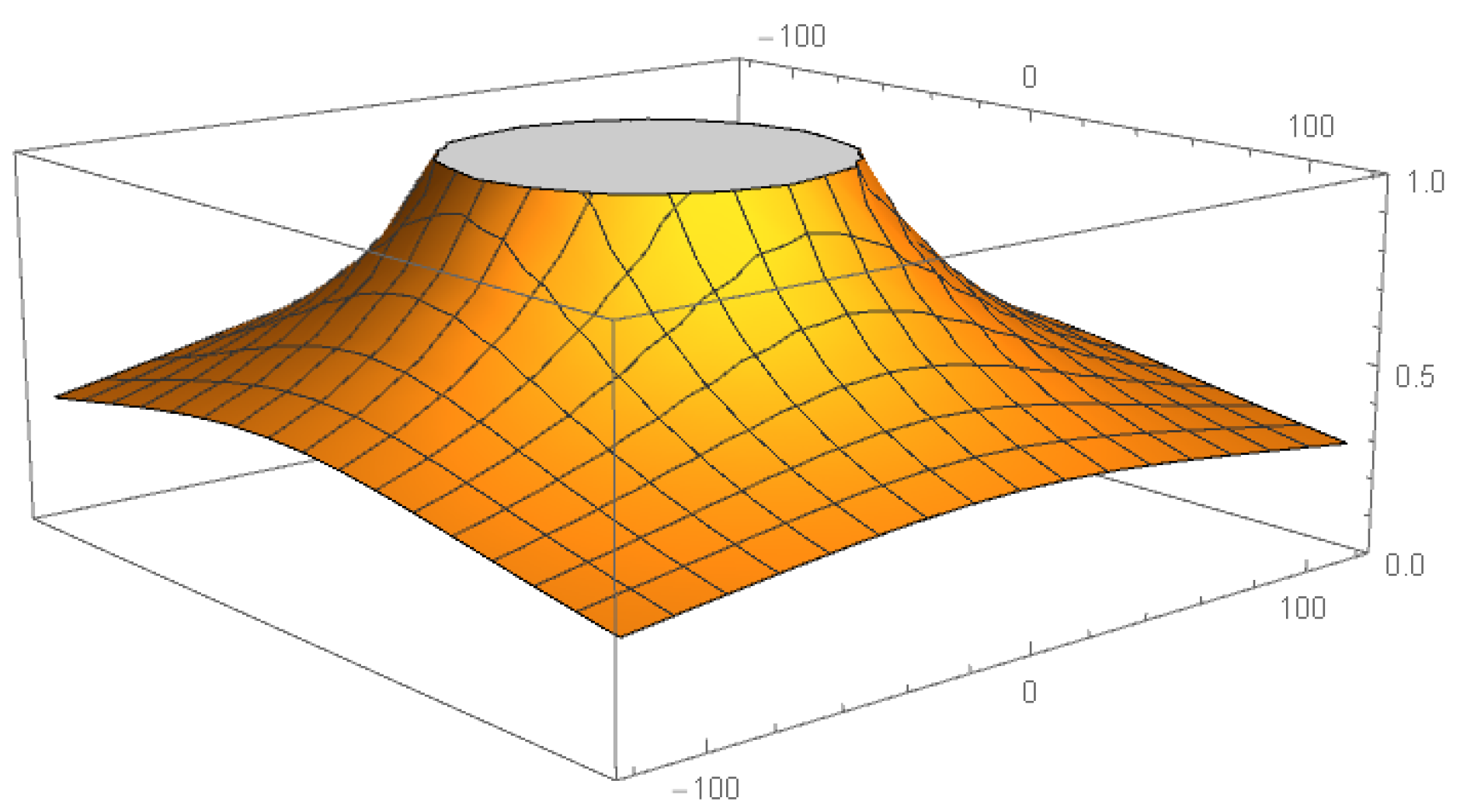
In Figure 1, the stability function of $z=1$ can be observed. It can be noticed that complex values of $\alpha$ inside the region $\left|z+\frac{135}{8}\right|<54$ define fourth-order iterative schemes, whose numerical performance do not include divergence.

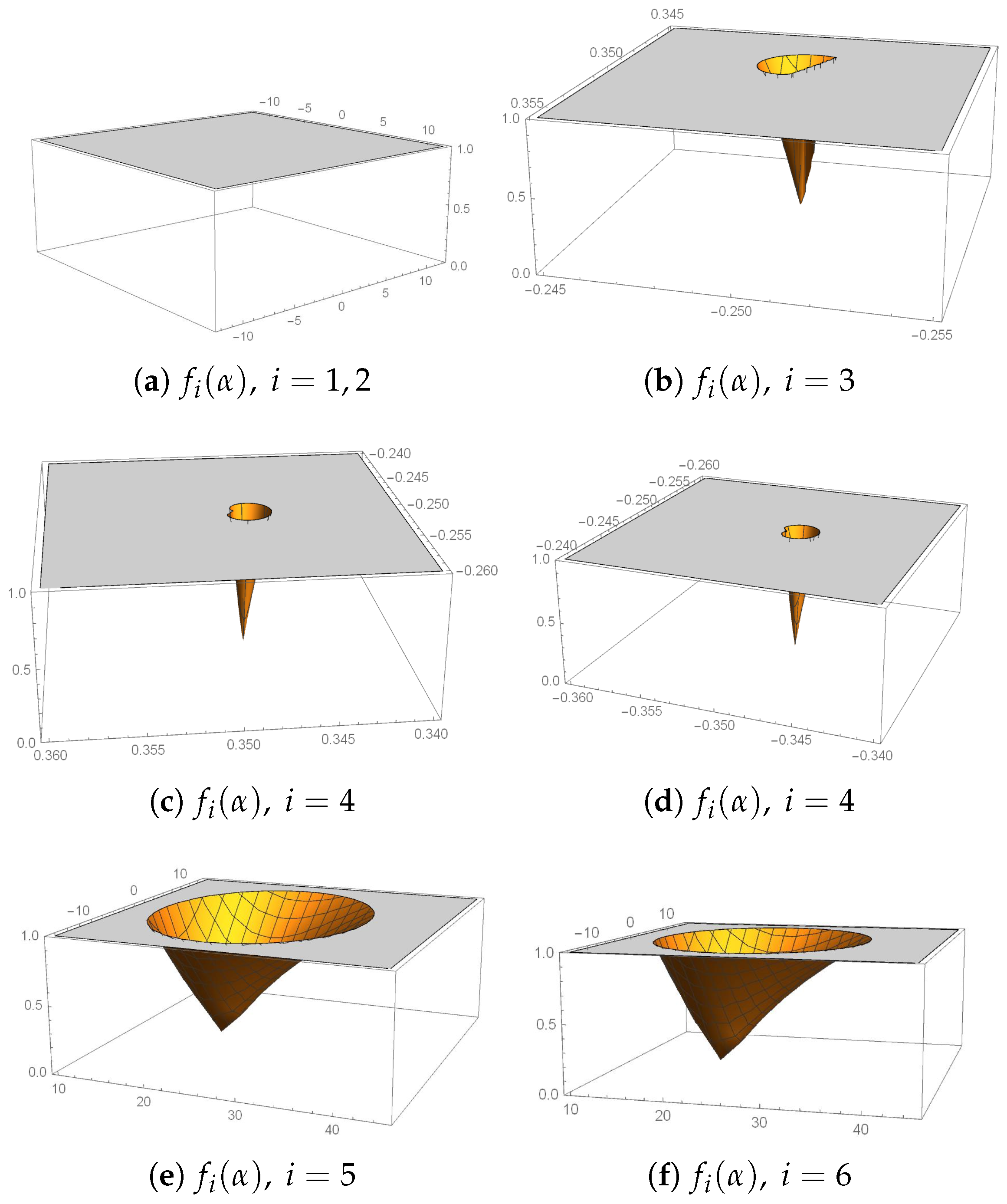
The demonstration of this result is similar to those of Theorem 2. In Figure 2, the set of stability regions of strange fixed points $f_1\left(\alpha \right)$ to $f_6\left(\alpha \right)$ appear.

Proposition 1.

The roots of$F\left(t\right)=27+189t+567t^2+(810-64\alpha )t^3+567t^4+189t^5+27t^6$are strange fixed points of$O_{\alpha }\left(z\right)$, different from $z=1$, and are denoted by $f_i\left(\alpha \right)$, $i=1,2,\dots ,6$. These strange fixed points are reduced to four if$\alpha =\frac{297}{8}$, as$f_1\left(\frac{297}{8}\right)=f_2\left(\frac{297}{8}\right)=1$. For$\alpha \ne \frac{297}{8}$,

• $f_1\left(\alpha \right)$and$f_2\left(\alpha \right)$are conjugate and repulsive, with independence of the value of parameter α.
• $f_3\left(\alpha \right)$and$f_4\left(\alpha \right)$are attractors for values of α in small regions of the complex plane, inside the complex area$[-0.26,-0.24]\times [-0.36,-0.34]$and$[-0.26,-0.24]\times [0.34,0.36]$. Moreover, both are superattracting for$\alpha \approx -0.250121\pm 0.348771i$.
• $f_5\left(\alpha \right)$and$f_6\left(\alpha \right)$are conjugate and attractors for values of α inside the complex area$[10,40]\times [-15,15]$. Moreover, both are superattracting for$\alpha \approx 20.3811$.

3.2. Critical Points and Parameter Planes

In order to determine the critical points, we calculate the first derivative of $O_{\alpha }\left(z\right)$,

$$\begin{array}{c}\hfill O_{\alpha }^{\prime }\left(z\right)={\displaystyle \frac{108z^3(135{(1+z)}^8+32\alpha {(1+z)}^6(2-3z+2z^2))}{{(27+162z+378z^2+378z^3+(135+64\alpha )z^4)}^2}}.\end{array}$$

By definition, the roots of $O_{\alpha }^{\prime }\left(z\right)=0$ are called critical points. As the order of convergence of our class of proposed iterative methods is higher than two, those fixed points coming from the original roots of the polynomial, that is, $z=0$ and $z=\infty$, are also critical points. In the next result, the rest of critical points are determined (called free critical points).

Proposition 2.

The number of free critical points of operator$O_{\alpha }\left(z\right)$is:

• One, if$\alpha =0$or$\alpha =-\frac{135}{8}$. In these cases, the reduced rational operator is:

  $$\begin{array}{ccc}\hfill O_{-\frac{135}{8}}\left(z\right)& =& \frac{x^4\left(27x^4+162x^3+378x^2+378x-945\right)}{-945x^4+378x^3+378x^2+162x+27},\hfill \\ \hfill O_0\left(z\right)& =& \frac{x^4\left(27x^4+162x^3+378x^2+378x+135\right)}{135x^4+378x^3+378x^2+162x+27},\hfill \end{array}$$

  whose only free critical point is$z=-1$, that is a pre-image of$z=1$.
• Three, if$\alpha \ne 0$and$\alpha \ne -\frac{135}{8}$, as in this case, they are defined as:

  $$\begin{array}{ccc}\hfill c{r}_1\left(\alpha \right)& =& -1,\hfill \\ \hfill c{r}_2\left(\alpha \right)& =& {\displaystyle \frac{-135+48\alpha -4\sqrt{14}\sqrt{-135\alpha -8{\alpha }^2}}{135+64\alpha }},\hfill \\ \hfill c{r}_3\left(\alpha \right)& =& {\displaystyle \frac{-135+48\alpha +4\sqrt{14}\sqrt{-135\alpha -8{\alpha }^2}}{135+64\alpha }}.\hfill \end{array}$$

It is easy to prove that $c{r}_2\left(\alpha \right)={\displaystyle \frac{1}{c{r}_3\left(\alpha \right)}}$. Therefore, $c{r}_2\left(\alpha \right)=c{r}_3\left(\alpha \right)=-1$ when $-135\alpha -8{\alpha }^2=0.$

As we have said, a classical result states that there is at least one critical point related with each basin of attraction. As $z=0$ and $z=\infty$ are both superattracting fixed points of $O_{\alpha }\left(z\right)$, they also are critical points and give rise to their respective Fatou components. For the other critical points, we can establish the following remarks:

(a)

If $\alpha =0$, then $c{r}_2=c{r}_3=-1$, and it is a pre-image of the fixed point $z=1$: $O_0\left(-1\right)=1$. As $z=1$ is repulsive for $\alpha =0$, $z=-1\in \mathcal{J}\left(O_{\alpha }\right)$. Thus, $O_p\left(z\right)$ has only two invariant Fatou components, $\mathcal{A}\left(0\right)$ and $\mathcal{A}\left(\infty \right)$.

(b)

If $\alpha =-{\displaystyle \frac{135}{8}}$, then $c{r}_2=c{r}_3=-1$, and $O_{-\frac{135}{8}}\left(-1\right)=1$. As $z=1$ is not a fixed point when $\alpha =-{\displaystyle \frac{135}{8}}$, then $z=-1\in \mathcal{J}\left(O_{\alpha }\right)$ and its orbit will remain at Julia set until the rounding error makes it fall into the basin of attraction of $z=0$ or $z=\infty$.

(c)

For the rest of the values of $\alpha \in \mathbf{C}$, we gave three critical points.

As we have previously stated, the dynamical performance of operator $O_{\alpha }\left(z\right)$ depends on the values of the parameter $\alpha$. In Figure 3, we can observe the parameter space associated with family (5): each point of the parameter plane is associated with a complex value of $\alpha$, i.e., with an element of family (5). A free critical point is employed as the starting point and, if for an specific value of $\alpha$, this critical point converges to $z=0$ or $z=\infty$, and then the point representing the value of $\alpha$ is painted in red color. Those values of $\alpha$ that make the critical point not converge to $z=0$ or $z=\infty$ are painted in black color. Therefore, each connected component of the parameter plane gives us subfamilies of procedures of class (5) with similar performance. The fractal defined as the boundary of these connected components separates regions of stable and unstable performance.

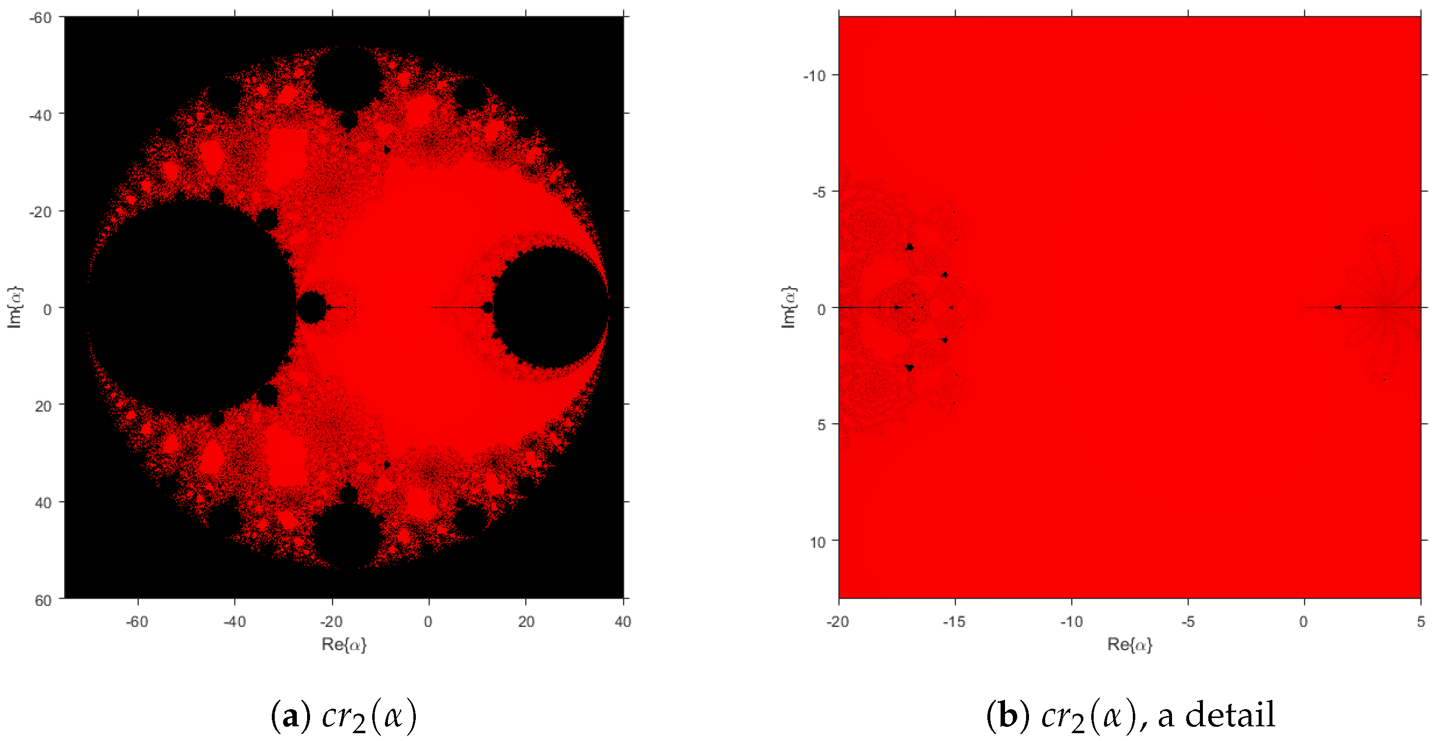
In Figure 3, the parameter plane associated with $c{r}_2={\displaystyle \frac{1}{c{r}_3}}$ is presented. Both critical points have the same parameter plane, as the are conjugated; thus, only one of them is considered a free independent critical point. It is usual not to plot a parameter plane for $z=-1$ as, although it is also a critical point, it is a pre-image of a fixed point and this plane would give us information only about the stability of fixed point $z=1$. We would like to remark that the outer black area corresponds to the stability of $z=1$. Moreover, the right-sided black circle inside the red area corresponds to the values of the parameter where $f_5\left(\alpha \right)$ and $f_6\left(\alpha \right)$ are simultaneously attracting. In the detail in Figure 3b, the end of both inner antennas can be observed and also, in red color, the wide area of stable values of $\alpha$, where only the convergence to the roots is possible. This parameter plane has been obtained by using a mesh of $500\times 500$ points for complex values of $\alpha$ and a maximum of 200 iterations.

3.3. Dynamical Planes

If one of the values of $\alpha$ (being painted red or black in the parameter plane) is selected, an specific member of the class of iterative methods (5) is chosen. Then, a set of initial estimations can be used in order to observe the performance of this iterative method.

The dynamical plane obtained by iterating an element of the family under study, is obtained by using each point of a mesh of $400\times 400$ points of the complex plane as an initial estimation. Those points with orbits converging to infinity appear in blue color; those that converge to zero are painted in orange (both with a precision of ${10}^{-3}$) and in green, red, etc., those converge in to other fixed points. All the fixed points appear as white stars in the figures when they are attractors or as white circles when they are repulsors. Moreover, the point is painted in black if the maximum number of 80 iterations is reached without converging to any of the fixed points. The routines used are slight modifications of those appearing in [24].

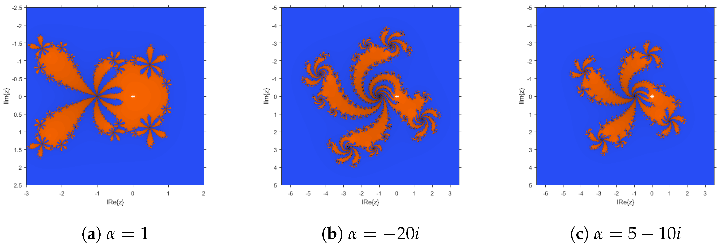
Thus, various stable elements can be chosen: values of $\alpha$ where no attracting periodic points nor strange fixed points appear. Some of them can be observed at the dynamical planes of Figure 4. In particular, Figure 4a, shows the performance of the method corresponding to $\alpha =1$, where the only basins of attraction are those of $z=0$ (orange area) and $z=\infty$ (blue region). Indeed, these basins are wider in this case than in cases $\alpha =-20i$ (Figure 4b) and $\alpha =5-10i$ (Figure 4c).

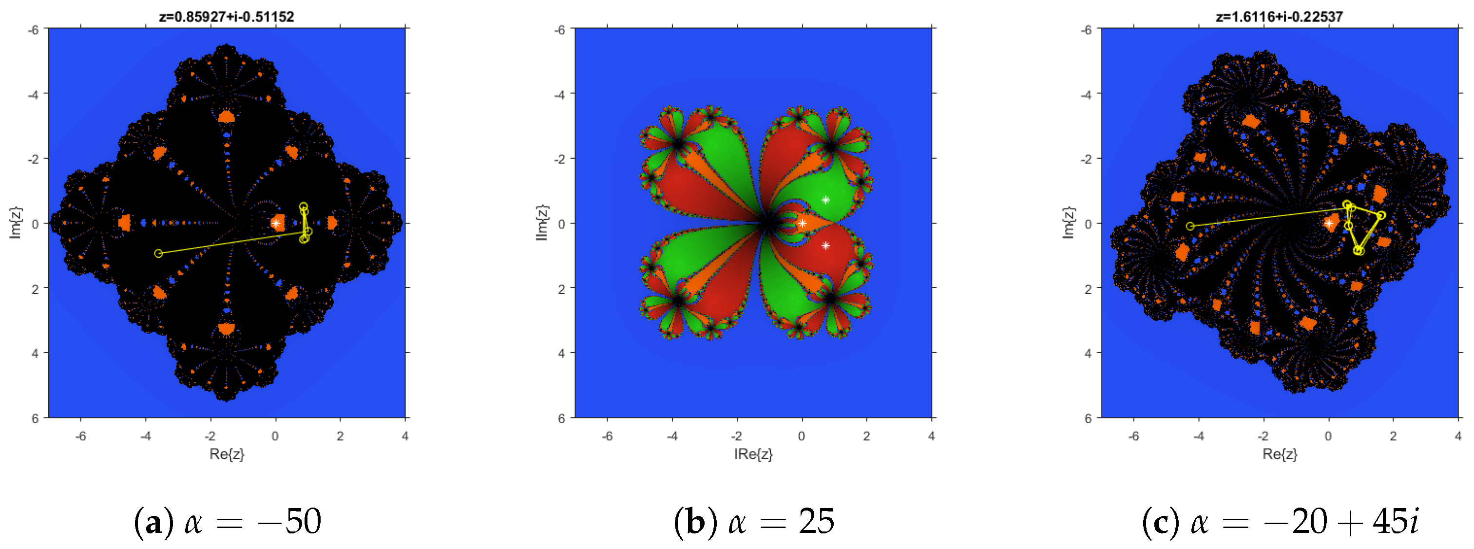
Similarly, some unstable elements can be chosen. It can be observed that $\alpha =-50$, which yields in the biggest black area of parameter plane (see Figure 3), corresponds to an iterative method whose bigger basin of attraction is that of an attracting 2-periodic orbit, which can be observed in yellow in Figure 5a. However, Figure 5b, where $\alpha =25$, the basins of attraction of attracting strange fixed points $f_5\left(\alpha \right)$ and $f_6\left(\alpha \right)$ appear in red and green, and are wider than the one of $z=0$. Other attracting elements appear for different values of the parameter; for example, $\alpha =-20+45i$ gives rise to a dynamical plane (see Figure 5c) where the black basin corresponds to an attracting periodic orbit of period four, which has been plotted in yellow in the figure. Therefore, it can be observed that the fractal defined by the Julia set, the boundary among the basins of attraction, is much more complicated in the case of unstable elements of the family of iterative methods.

This information will be checked numerically in the next section, where non-polynomial functions are used to see the performance of some of these stable and unstable elements of the proposed family of iterative methods.

4. Numerical Results

In this section, we demonstrate the behaviour of the new family of iterative methods defined in (5), which is a particular sub-class of the method defined in (3). From the stability analysis, we know that those members of this class of iterative schemes, corresponding to values of $\alpha$ inside the red area of the parameter plane (see Figure 3), have better performance on quadratic polynomials than those belonging to black areas. We check now their performance on other kind of functions in order to see whether these stability properties are held.

Numerical computations have been carried out by using $MATLAB$ R2019a, by using variable precision arithmetics with 1000 digits of mantissa, on a PC equipped with a $Intel$ Core™ i5-5200U CPU 2.20GHz. In all the tables, we demonstrate the residuals $\left|f\right(x_{k+1}\left)\right|$ and $|x_{k+1}-x_k|$ at the last iteration, the estimation of the solution found, the number of iterations needed (if the scheme does not converge, a “d” appears) and the execution time in seconds with the format $t\pm d$, calculated with the command cputime. In it, t is the mean of 100 consecutive executions and d is the standard deviation. The stopping criterion used is $|x_{k+1}-x_k|+|f\left(x_{k+1}\right)|<{10}^{-200}$, and the ACOC, defined in [26], has been also presented in the tables, whose expression is:

$$ACOC=\frac{\ln |(x_{k+1}-x_k)/(x_k-x_{k-1})|}{\ln |(x_k-x_{k-1})/(x_{k-1}-x_{k-2})|},k=2,3,\dots$$

The nonlinear test functions used are both academical and real-life functions:

• $f_1\left(x\right)=si{n}^{2}x-x^2+1$, with two real roots at $x_1^{*}\approx$$-1.4044$ and $x_2^{*}\approx 1.4044$.
• $f_2\left(x\right)=cosx-x{e}^x$, with real roots at $x_1^{*}\approx 0.517$, $x_2^{*}\approx -14.137$ and $x_3^{*}\approx -17.278$, among others.
• Colebrook-White function [27] $f_3\left(x\right)=\sqrt{\frac{1}{f}}+0.86\ln \left(\frac{{10}^{-4}}{3.7}+\frac{2.51}{{10}^5\sqrt{\frac{1}{f}}}\right)$, with a real root at $x^{*}\approx 0.01885050$, among others.

Colebrook-White function is one of the most accurate equations for the calculation of the friction factor and over a wider range, but it has the disadvantage of complexity, as it is an implicit function. It must be solved iteratively until an acceptable level of error is reached, with the computational cost and time involved. It was proposed by Colebrook and White in 1939 [4,27]. and is the most widely used because it is the most accurate and universal. For each nonlinear function, two initial approximations are used: one near to the solution and the other far from it.

Some of the proposed schemes are compared with classical Newton’ and Jarratt’s methods, Wang. et al. scheme KM [28] and two procedures from Chun [29], denoted by CM1 and CM2.

In

Table 1. $f_1\left(x\right)=si{n}^{2}x-x^2+1$, $x_0=2$.

$\mathit{\alpha }$	$\left|\mathit{f}\right({\mathit{x}}_{\mathit{k}+1}\left)\right|$	$|{\mathit{x}}_{\mathit{k}+1}-{\mathit{x}}_{\mathit{k}}|$	Solution	Iterations	ACOC	Time (s)
−50	7.0883 $\times {10}^{-1007}$	8.4884 $\times {10}^{-253}$	−1.4044	8	4.0	0.3223 ± 0.2001
−40	0	1.4357 $\times {10}^{-402}$	−1.4044	29	4.0	0.9086 ± 0.5325
−20 + 45i	d	d	d	d	d	d
−16 − 45i	2.4842 $\times {10}^{-1432}$	5.1013 $\times {10}^{-425}$	1.4044	10	4.0	0.3597 ± 0.1498
1	0	1.8974 $\times {10}^{-331}$	1.4044	6	4.0	0.2188 0.2253 ± 0.0838
−20i	7.0302 $\times {10}^{-1505}$	8.8753 $\times {10}^{-498}$	1.4044	7	4.0	0.2487 ± 0.0415
5 − 10i	0.0	1.4936 $\times {10}^{-755}$	1.4044	7	4.0	0.2481 0.2419 ± 0.0176
−4.5 + 10i	3.5457 $\times {10}^{-891}$	1.0501 $\times {10}^{-223}$	1.4044	6	4.0	0.2223 ± 0.0224
$Newton$	1.4479 $\times {10}^{-514}$	8.6274 $\times {10}^{-258}$	1.4044	10	2.0	0.2033 ± 0.0248
$Jarratt$	0.0	9.6997 $\times {10}^{-510}$	1.4044	6	4.0	0.1970 ± 0.0200
$CM1$	0.0	4.9393 $\times {10}^{-810}$	1.4044	5	6.0	0.2264 ± 0.0419
$CM2$	0.0	1.5533 $\times {10}^{-693}$	1.4044	5	6.0	0.2334 ± 0.0619
$KM$	0.0	9.821 $\times {10}^{-761}$	1.4044	5	6.0	0.2158 ± 0.0185

and

Table 2. $f_1\left(x\right)=si{n}^{2}x-x^2+1$, $x_0=4$.

$\mathit{\alpha }$	$\left|\mathit{f}\right({\mathit{x}}_{\mathit{k}+1}\left)\right|$	$|{\mathit{x}}_{\mathit{k}+1}-{\mathit{x}}_{\mathit{k}}|$	Solution	Iterations	ACOC	Time (s)
−50	0	1.5957 $\times {10}^{-569}$	1.4044	7	4.0	0.2347 ± 0.0293
−40	0	3.5896 $\times {10}^{-451}$	1.4044	7	4.0	0.2420 ± 0.0614
−20 + 45i	1.1188 $\times {10}^{-1416}$	1.475 $\times {10}^{-409}$	1.4044	8	4.0	0.2589 ± 0.0262
−16 − 45i	2.9743 $\times {10}^{-1380}$	8.4532 $\times {10}^{-372}$	1.4044	8	4.0	0.2603 ± 0.0305
1	0	7.1697 $\times {10}^{-507}$	1.4044	7	4.0	0.2263 ± 0.0155
−20i	1.1363 $\times {10}^{-995}$	6.6845 $\times {10}^{-250}$	1.4044	7	4.0	0.2347 ± 0.0266
5 − 10i	3.0563 $\times {10}^{-1262}$	2.6576 $\times {10}^{-316}$	1.4044	7	4.0	0.2314 ± 0.0152
−4.5 + 10i	0	3.7277 $\times {10}^{-384}$	1.4044	7	4.0	0.2302 ± 0.0129
$Newton$	1.6796 $\times {10}^{-543}$	2.9384 $\times {10}^{-272}$	1.4044	11	2.0	0.2013 ± 0.0128
$Jarratt$	0.0	1.7167 $\times {10}^{-754}$	1.4044	7	4.0	0.1970 ± 0.0200
$CM1$	0.0	7.3559 $\times {10}^{-390}$	1.4044	5	6.0	0.2177 ± 0.0203
$CM2$	0.0	2.2786 $\times {10}^{-230}$	1.4044	5	6.0	0.2100 ± 0.0144
$KM$	0.0	9.2909 $\times {10}^{-265}$	1.4044	5	6.0	0.2083 ± 0.0436

, we notice that when values of $\alpha$ are considered inside the stable zone ($\alpha =1$, $\alpha =-20i$, $\alpha =5-10i$ or $\alpha =-4.5+10i$), the method achieves better approximations to any of the roots with fewer iterations. It is noteworthy that one of the unstable values of the parameter, $\alpha =-20+45i$, does not even obtain convergence. One of the stable members for $\alpha =1$, shows the lowest execution time, even compared with the classical Newton and Jarratt’s methods.

In

Table 3. $f_2\left(x\right)=cosx-x{e}^x$, $x_0=1$.

$\mathit{\alpha }$	$\left|\mathit{f}\right({\mathit{x}}_{\mathit{k}+1}\left)\right|$	$|{\mathit{x}}_{\mathit{k}+1}-{\mathit{x}}_{\mathit{k}}|$	Solution	Iterations	ACOC	Time (s)
−50	1.0082 $\times {10}^{-1007}$	4.6325 $\times {10}^{-399}$	−14.137	8	4.0	0.2728 ± 0.0657
−40	d	d	d	d	d	d
−20 + 45i	2.9787 $\times {10}^{-1009}$	2.2945 $\times {10}^{-324}$	−17.278	12	4.0	0.3858 ± 0.0756
−16 − 45i	d	d	d	d	d	d
1	0	5.7578 $\times {10}^{-315}$	0.517	6	4.0	0.2247 ± 0.0474
−20i	1.9236 $\times {10}^{-1366}$	6.3944 $\times {10}^{-359}$	0.517	7	4.0	0.2566 ± 0.0551
5 − 10i	0.0	6.7181 $\times {10}^{-632}$	0.517	7	4.0	0.2797 ± 0.0715
−4.5 + 10i	3.0281 $\times {10}^{-1747}$	1.7704 $\times {10}^{-740}$	0.517	7	4.0	0.3034 ± 0.0963
$Newton$	1.4521 $\times {10}^{-498}$	7.5503 $\times {10}^{-250}$	0.517	10	2.0	0.2075 ± 0.0499
$Jarratt$	0.0	3.9685 $\times {10}^{-570}$	0.517	6	4.0	0.2198 ± 0.0529
$CM1$	0.0	4.9393 $\times {10}^{-810}$	1.4044	5	6.0	0.1923 ± 0.0152
$CM2$	0.0	1.5533 $\times {10}^{-693}$	1.4044	5	6.0	0.1922 ± 0.0168
$KM$	0.0	9.821 $\times {10}^{-761}$	1.4044	5	6.0	0.2158 ± 0.0185

and

Table 4. $f_2\left(x\right)=cosx-x{e}^x$, $x_0=2.4$.

$\mathit{\alpha }$	$\left|\mathit{f}\right({\mathit{x}}_{\mathit{k}+1}\left)\right|$	$|{\mathit{x}}_{\mathit{k}+1}-{\mathit{x}}_{\mathit{k}}|$	Solution	Iterations	ACOC	Time (s)
−50	1.4177 $\times {10}^{-1008}$	5.6457 $\times {10}^{-294}$	−1.8639	6	4.0	0.1848 ± 0.0133
−40	1.4177 $\times {10}^{-1008}$	5.1924 $\times {10}^{-678}$	−1.8639	7	4.0	0.2048 ± 0.0155
−20 + 45i	d	d	d	d	d	d
−16 − 45i	d	d	d	d	d	d
1	0	1.6078 $\times {10}^{-702}$	0.5177	8	4.0	0.2273 ± 0.0189
−20i	1.0214 $\times {10}^{-961}$	1.0043 $\times {10}^{-240}$	−1.8639	9	4.0	0.2553 ± 0.0230
5 − 10i	0.0	4.4053 $\times {10}^{-627}$	0.5177	22	4.0	0.5289 ± 0.0233
−4.5 + 10i	1.4234 $\times {10}^{-979}$	2.2838 $\times {10}^{-242}$	−29.8451	9	4.0	0.2653 ± 0.0487
$Newton$	2.4269 $\times {10}^{-437}$	3.0867 $\times {10}^{-219}$	0.5177	12	2.0	0.1956 ± 0.0260
$Jarratt$	0.0	1.0119 $\times {10}^{-612}$	0.5177	7	4.0	0.1909 ± 0.0243
$CM1$	0.0	4.8037 $\times {10}^{-559}$	0.5177	6	6.0	0.2230 ± 0.0273
$CM2$	0.0	1.5709 $\times {10}^{-609}$	0.5177	6	6.0	0.2208 ± 0.0261
$KM$	0.0	9.7594 $\times {10}^{-581}$	0.5177	5	6.0	0.2106 ± 0.0218

, the best results are obtained by the stable proposed members of family (5), in terms of the number of iterations and residuals. Two of the unstable members do not reach convergence to any root.

In the case of the Colebrook-White function, as shown in

Table 5. $f_3\left(x\right)=\sqrt{\frac{1}{f}}+0.86\ln \left(\frac{{10}^{-4}}{3.7}+\frac{2.51}{{10}^5\sqrt{\frac{1}{f}}}\right)$, $x_0=0.02$.

$\mathit{\alpha }$	$\left|\mathit{f}\right({\mathit{x}}_{\mathit{k}}\left)\right|$	$|{\mathit{x}}_{\mathit{k}+1}-{\mathit{x}}_{\mathit{k}}|$	Solution	Iterations	ACOC	Time (s)
−50	2.2683 $\times {10}^{-1007}$	5.9163 $\times {10}^{-668}$	0.01885050	6	4.0	0.4098 ± 0.1367
−40	1.1341 $\times {10}^{-1007}$	3.1316 $\times {10}^{-702}$	0.01885050	6	4.0	0.3978 ± 0.0532
−20 + 45i	2.4166 $\times {10}^{-667}$	0.0	0.01885050	6	4.0	0.4517 ± 0.1145
−16 − 45i	1.5247 $\times {10}^{-1677}$	1.4073 $\times {10}^{-671}$	0.01885050	6	4.0	0.4555 ± 0.0999
1	1.1341 $\times {10}^{-1007}$	2.2713 $\times {10}^{-277}$	0.01885050	5	4.0	0.3361 ± 0.0419
−20i	4.0218 $\times {10}^{-796}$	9.0943 $\times {10}^{-202}$	0.01885050	5	4.0	0.3386 ± 0.0255
5 − 10i	1.5202 $\times {10}^{-872}$	8.1035 $\times {10}^{-221}$	0.01885050	5	4.0	0.3744 ± 0.0241
−4.5 + 10i	3.2812 $\times {10}^{-893}$	5.7307 $\times {10}^{-226}$	0.01885050	5	4.0	0.3706 ± 0.0178
$Newton$	2.9268 $\times {10}^{-693}$	5.9571 $\times {10}^{-349}$	0.01885050	9	2.0	0.3630 ± 0.0332
$Jarratt$	1.1341 $\times {10}^{-1007}$	2.0266 $\times {10}^{-489}$	0.01885050	5	4.0	0.3319 ± 0.0655
$CM1$	1.1341 $\times {10}^{-1007}$	2.0266 $\times {10}^{-489}$	0.01885050	5	4.0	0.3447 ± 0.0301
$CM2$	1.1341 $\times {10}^{-1007}$	2.0266 $\times {10}^{-489}$	0.01885050	5	4.0	0.3494 ± 0.0252
$KM$	1.1341 $\times {10}^{-1007}$	2.0266 $\times {10}^{-489}$	0.01885050	5	4.0	0.3400 ± 0.0208

and

Table 6. $f_3\left(x\right)=\sqrt{\frac{1}{f}}+0.86\ln \left(\frac{{10}^{-4}}{3.7}+\frac{2.51}{{10}^5\sqrt{\frac{1}{f}}}\right)$, $x_0=0.009$.

$\mathit{\alpha }$	$\left|\mathit{f}\right({\mathit{x}}_{\mathit{k}}\left)\right|$	$|{\mathit{x}}_{\mathit{k}+1}-{\mathit{x}}_{\mathit{k}}|$	Solution	Iterations	ACOC	Time (s)
−50	d	d	d	d	d	d
−40	d	d	d	d	d	d
−20 + 45i	d	d	d	d	d	d
−16 − 45i	d	d	d	d	d	d
1	2.3085 $\times {10}^{-906}$	4.1347 $\times {10}^{-229}$	0.01885050	6	4.0	0.3880 ± 0.0206
−20i	2.2683 $\times {10}^{-1007}$	1.9203 $\times {10}^{-445}$	0.01885050	9	4.0	0.6564 ± 0.0519
5 − 10i	1.2533 $\times {10}^{-1118}$	2.48 $\times {10}^{-282}$	0.01885050	7	4.0	0.5059 ± 0.0328
−4.5 + 10i	2.2683 $\times {10}^{-1007}$	2.5742 $\times {10}^{-397}$	0.01885050	7	4.0	0.5020 ± 0.0177
$Newton$	2.0584 $\times {10}^{-397}$	4.9958 $\times {10}^{-201}$	0.01885050	10	2.0	0.3942 ± 0.0227
$Jarratt$	1.1341 $\times {10}^{-1007}$	1.1036 $\times {10}^{-272}$	0.01885050	5	4.0	0.3200 ± 0.0233
$CM1$	0	1.8787 $\times {10}^{-675}$	0.01885050	5	6.0	0.4191 ± 0.0255
$CM2$	0	1.8799 $\times {10}^{-675}$	0.01885050	5	6.0	0.4194 ± 0.0354
$KM$	0	1.8793 $\times {10}^{-675}$	0.01885050	5	6.0	0.4064 ± 0.0168

, it is only possible to converge to the solution with a very close initial estimation. In this case, the best results in terms of the number of iterations are obtained by the stable members of the proposed class as well as by Jarratt’s method. In terms of the lowest execution time, the best results are given by Jarratt and $\alpha =1$ schemes.

5. Conclusions

In this manuscript, we present a new parametric family of iterative methods with the fourth-order of convergence in order to solve nonlinear equations $f\left(x\right)=0$. The class has been generated using composition and weight functions techniques. With the help of dynamical analysis, we select the most stable methods by choosing some values of the free parameter. These schemes demonstrate a simple fractal as the Julia set separating the basins of attraction. The described numerical examples allow us to confirm the theoretical results corresponding to the proposed convergence and stability. On the other hand, when the parameter alpha is unstable, the corresponding method needs more iterations to converge or fails to converge. These numerical tests confirm that the new family of methods is suitable for solving nonlinear problems, when the adequate values of the free disposable parameter are used.