Modal Shifted Fifth-Kind Chebyshev Tau Integral Approach for Solving Heat Conduction Equation

Abstract

In this study, a spectral tau solution to the heat conduction equation is introduced. As basis functions, the orthogonal polynomials, namely, the shifted fifth-kind Chebyshev polynomials (5CPs), are used. The proposed method’s derivation is based on solving the integral equation that corresponds to the original problem. The tau approach and some theoretical findings serve to transform the problem with its underlying conditions into a suitable system of equations that can be successfully solved by the Gaussian elimination method. For the applicability and precision of our suggested algorithm, some numerical examples are given.

1. Introduction

The heat equation pioneered by Fourier [1] describes the distribution of heat in a given body over time [2], which is a type of second-order parabolic partial differential equation. It has many applications in diverse scientific fields. Moreover, it has been studied analytically and numerically. For example, Meyu and Koriche [3] proposed two techniques based on the separation of variables and finite-difference methods to solve the heat equation in one dimension. Liu and Chang [4] used a method of nonlocal boundary shape functions to solve a nonlinear heat equation with nonlocal boundary conditions. Tassaddiq et al. [5] introduced an approximate approach based on a cubic B-spline collocation method to solve the heat equation with classical and nonclassical boundary conditions.

It is well-known that obtaining accurate and efficient methods for solving differential equations has become an important research point. There are several analytic and numerical methods, such as the homotopy analysis method [6,7], the variational iteration method [8,9], the Adomian decomposition method [10,11], the finite-difference method [12,13,14], the finite-element method [15,16,17], and spectral methods [18,19,20,21,22]. Spectral methods have many advantages if compared with the other methods because they yield exponential rate convergence, a good accuracy, and the computational efficiency of the solutions while failing for many complicated problems with singular solutions. Thus, it is relevant to be interested in how to enlarge the adaptability of spectral methods and construct certain simple approximation schemes without a loss of accuracy for more complicated problems. Further applications of spectral methods in different disciplines may be found in [23,24,25,26,27,28,29].

Orthogonal polynomials, such as Legendre polynomials and Chebyshev polynomials, have received a lot of attention from both theoretical and practical perspectives [30,31,32]. Chebyshev polynomials have been used as an important category of basis functions to solve ordinary, partial, and fractional differential equations, see for instance [33,34,35,36,37,38]. Two major reasons for the widespread use of these polynomials are the high accuracy of the approximation and the simplicity of numerical methods established based on these polynomials. There are six types of Chebyshev polynomials, they are Chebyshev polynomials of the first, second, third, fourth, fifth, and sixth kind. All the kinds of Chebyshev polynomials have their important parts in numerical analysis and approximation theory. There are old and recent contributions regarding the first four kinds, see, for example, [39,40], while the fifth and sixth kind of Chebyshev polynomials have gained recently a fast-growing attention from many authors. For instance, Sadri and Aminikhah in [41] treated a multiterm variable-order time-fractional diffusion-wave equation using a new efficient algorithm based on the $5CPs$. Moreover, Abd-Elhameed and Youssri in [42] employed the $5CPs$ for solving the convection–diffusion equation.

The following items are the main goals of this paper:

• Deriving new theorems, corollaries, and lemmas concerned with the shifted $5CPs$ that serve in the derivation of our proposed numerical scheme.
• Presenting a new spectral tau algorithm for the numerical treatment of the heat conduction equation.
• Investigating the convergence analysis of the proposed double-shifted Chebyshev expansion.
• Performing some comparisons to clarify the efficiency and accuracy of our method.

To the best of our knowledge, some advantages of the proposed technique can be mentioned as follows:

• By choosing the shifted $5CPs$ as basis functions, and taking a few terms of the retained modes, it is possible to produce approximations with excellent precision. Less calculation is required. In addition, the resulting errors are small.
• In comparison to other Chebyshev polynomials, the shifted $5CPs$ are not as well-studied or used. This motivates us to find theoretical findings concerning them. Furthermore, we found that the obtained numerical results, if they are used as basis functions, are satisfactory.

We point out here that the novelty of our contribution in this paper can be listed as follows:

• Some derivatives and integral formulas of the shifted $5CPs$ are given in reduced formulas that do not involve any hypergeometric forms.
• The employment of these basis functions to the numerical treatment of the heat conduction equation is new.

The contents of the paper are arranged as follows. Section 2 is devoted to presenting mathematical preliminaries containing some relevant properties of $5CPs$ and their shifted ones. In addition, some new formulas concerning the shifted $5CPs$ are derived. In Section 3, we present and implement a spectral tau method for solving the heat conduction equation based on employing the shifted $5CPs$. In Section 4, we investigate in detail the convergence and error analysis of the suggested shifted $5CPs$. In Section 5, some numerical examples are given to ensure the efficiency, simplicity, and applicability of the suggested method. Finally, conclusions are reported in Section 6.

2. An Account on the Shifted $5CPs$ and Some New Useful Formulas

This section is confined to presenting an account on the $5CPs$, $X_j\left(t\right)$, $j\ge 0$, and their shifted ones. In addition, building on some of their fundamental relations, we derive some new specific formulas that serve in the derivation of our proposed numerical scheme. More precisely, we establish the second-order derivative formulas of the shifted polynomials and also the corresponding integral formulas of these polynomials.

2.1. An Account on the Shifted $5CPs$

The $5CPs$$\left(X_i\left(t\right)\right)$ are a sequence of orthogonal polynomials on $[-1,1]$ (see, [28,43]) that satisfy the following orthogonality relation:

$${\int }_{-1}^1\frac{t^2}{\sqrt{1-t^2}}{X}_i\left(t\right)X_j\left(t\right)dt=h_i{\delta }_{i,j},$$

where

$$h_i=\frac{\pi }{2^{2i+1}}\left\{\begin{array}{cc}1,\hfill & \mathrm{i}\mathrm{f}i\mathrm{even},\hfill \\ \frac{i+2}{i},\hfill & \mathrm{i}\mathrm{f}i\mathrm{odd},\hfill \end{array}\right.$$

and

$${\delta }_{i,j}=\left\{\begin{array}{cc}1,\hfill & \mathrm{i}\mathrm{f}i=j,\hfill \\ 0,\hfill & \mathrm{i}\mathrm{f}i\ne j.\hfill \end{array}\right.$$

$X_i\left(t\right)$ may be generated with the aid of the following recursive formula:

$$X_i\left(t\right)=t{X}_{i-1}\left(t\right)-{\varrho }_i{X}_{i-2}\left(t\right),i\ge 2,$$

where $X_0\left(t\right)=1,X_1\left(t\right)=t$ and

$${\varrho }_i=\frac{{(i-1)}^2+i+{(-1)}^i(2i-1)}{4i(i-1)}.$$

The shifted orthogonal $5CPs$ on $[0,\tau ]$ are defined as

$$C_i\left(t\right)=X_i\left(\frac{2t}{\tau }-1\right),\tau >0,$$

with the orthogonality relation

$${\int }_0^{\tau }\omega \left(t\right)C_i\left(t\right)C_j\left(t\right)dt=h_{\tau ,i}{\delta }_{i,j},$$

(1)

where $h_{\tau ,i}={\tau }^2{h}_i$ and $\omega \left(t\right)=\frac{{(2t-\tau )}^2}{\sqrt{t\tau -t^2}}.$

Lemma 1

([28]). The analytic formula of $X_j\left(x\right)$ may be split to the following two analytic formulas:

$$\begin{array}{cc}\hfill X_{2i}\left(x\right)=& (2i+1)\sum _{n=0}^i\frac{{(-1)}^n{2}^{-2n}(2i-n)!}{n!(2i-2n+1)!}{x}^{2i-2n},i\ge 0,\hfill \end{array}$$

(2)

$$\begin{array}{cc}\hfill X_{2i+1}\left(x\right)=& \frac{\left(i+\frac{3}{2}\right)!}{(2i+1)!}\sum _{n=0}^i\frac{{(-1)}^n\left(\genfrac{}{}{0pt}{}{i}{i-n}\right)(2i-n+1)!}{\left(i-n+\frac{3}{2}\right)!}{x}^{2i-2n+1},i\ge 0.\hfill \end{array}$$

(3)

Theorem 1

([28]). The following two inversion formulas hold for the polynomials $X_j\left(x\right)$:

$$\begin{array}{cc}\hfill x^{2j}=& \sum _{r=0}^j\frac{\left(\genfrac{}{}{0pt}{}{2j+1}{r}\right)}{2^{2r}}{X}_{2j-2r}\left(x\right),j\ge 0,\hfill \end{array}$$

(4)

$$\begin{array}{cc}\hfill x^{2j+1}=& \left(j+\frac{3}{2}\right)!\sum _{r=0}^j\frac{(\genfrac{}{}{0pt}{}{j}{j-r})(2j-2r+2)!}{\left(j-r+\frac{3}{2}\right)!(2j-r+2)!}{X}_{2j-2r+1}\left(x\right),j\ge 0.\hfill \end{array}$$

(5)

2.2. Derivation of the Second-Order Derivative Formulas of $C_j\left(t\right)$

The following theorem exhibits the expressions of the second-order derivatives of $X_j\left(t\right)$ in terms of their original ones.

Theorem 2.

The second-order derivative of the polynomials $X_i\left(t\right)$ can be expressed explicitly as:

$$D^2{X}_{2i}\left(t\right)=\sum _{n=0}^i{4}^{-n}\left({(-1)}^n(-2i+2n+1)-(2i+1)\left(-2i(n+1)+n^2+n+1\right)\right)X_{2i-2n-2}\left(t\right),$$

(6)

$$D^2{X}_{2i+1}\left(t\right)=(2i+3)\sum _{n=0}^i\frac{2^{1-2n}(n-i)\left(\frac{{(-1)}^n\left(4{(i-n)}^2-1\right)}{4i(i+2)+3}-2i(n+1)+n^2\right)}{2i-2n+1}{X}_{2i-2n-1}\left(t\right).$$

(7)

Proof. 

First, we prove relation (6). The power-form representation of $X_i\left(t\right)$ in (2) enables one to express $D^2{X}_{2i}\left(t\right),$ in the following form:

$$D^2{X}_{2i}\left(t\right)=(2i+1)\sum _{n=0}^i\frac{{(-1)}^n{2}^{1-2n}(2i-2n-1)(i-n)(2i-n)!}{n!(2i-2n+1)!}{t}^{2i-2n-2},$$

which can be written with the aid of the inversion formula (4) as

$$\begin{array}{cc}\hfill D^2{X}_{2i}\left(t\right)=& (2i+1)\sum _{n=0}^i\frac{{(-1)}^n{2}^{1-2n}(2i-2n-1)(i-n)(2i-n)!}{n!(2i-2n+1)!}\hfill \\ & \times \sum _{r=0}^{i-n-1}\frac{\left(\genfrac{}{}{0pt}{}{2i-2n-1}{r}\right)}{2^{2r}}{X}_{2i-2n-2r-2}\left(t\right).\hfill \end{array}$$

The last relation after expanding and rearranging the terms can be converted into

$$\begin{array}{cc}\hfill D^2{X}_{2i}\left(t\right)=& (2i+1)\sum _{n=0}^i{4}^{-n}\hfill \\ & \times \sum _{r=0}^n\frac{{(-1)}^{n-r+1}(-2i+2n-2r+1)(2i-n+r)!}{\left(r\right)!(2i-2n+2r+1)(n-r)!(2i-2n+r-1)!}{X}_{2i-2n-2}\left(t\right).\hfill \end{array}$$

Now, in order to reduce the summation on the right-hand side of the last formula, set

$$G_{n,i}=\sum _{r=0}^n\frac{{(-1)}^{n-r+1}(-2i+2n-2r+1)(2i-n+r)!}{\left(r\right)!(2i-2n+2r+1)(n-r)!(2i-2n+r-1)!}.$$

The application of Zeilberger’s algorithm mentioned in [44] enables us to get the following recurrence relation for $G_{n,i}$:

$$\begin{array}{cc}\hfill & \left(4i^{2}n-6i{n}^2+2n^3+10i^2-26in+12n^2-29i+25n+18\right)G_{n,i}\hfill \\ & +\left(4i^2-4in+2n^2-4i+6n+1\right)G_{n+1,i}=0\hfill \\ & +\left(-4i^{2}n+6i{n}^2-2n^3-6i^2+14in-6n^2+9i-7n-3\right)G_{n+2,i}=0,\hfill \end{array}$$

(8)

with the initial values:

$$G_{0,i}=\frac{2i(2i-1)}{2i+1},G_{1,i}=\frac{2(4i^2-3)}{2i+1}.$$

The recurrence relation (8) can be exactly solved to give

$$G_{n,i}=2i(n+1)+\frac{{(-1)}^n(-2i+2n+1)}{2i+1}-n^2-n-1,$$

and therefore, relation (6) can be obtained.

Now, we prove Formula (7). Based on relation (3), we have

$$D^2{X}_{2i+1}\left(t\right)=\sum _{n=0}^i\frac{(2i+3){(-1)}^{n+1}{4}^{-n}(2i-n+1)!}{n!(-2i+2n-3)(2i-2n-1)!}{t}^{2i-2n-1}.$$

Making use of Formula (5) yields

$$\begin{array}{cc}\hfill D^2{X}_{2i+1}\left(t\right)=& \sum _{n=0}^i\frac{(2i+3){(-1)}^{n+1}{4}^{-n}(2i-n+1)!\left(i-n+\frac{1}{2}\right)!}{n!(-2i+2n-3)(2i-2n-1)!}\hfill \\ & \times \sum _{r=0}^{i-n-1}\frac{(2i-2n-2r)!\left(\genfrac{}{}{0pt}{}{i-n-1}{i-n-r-1}\right)}{(2i-2n-r)!\left(i-n-r+\frac{1}{2}\right)!}{X}_{2i-2n-2r-1}\left(t\right).\hfill \end{array}$$

The last relation after expanding and rearranging the terms can be converted into

$$\begin{array}{cc}\hfill D^2{X}_{2i+1}\left(t\right)=& \sum _{n=0}^i\frac{(2i+3)2^{1-2n}(n-i)}{2i-2n+1}\hfill \\ & \times \sum _{r=0}^n\frac{{(-1)}^{n-r}(-2i+2n-2r-1)(2i-n+r+1)!}{\left(r\right)!(2i-2n+2r+3)(n-r)!(2i-2n+r)!}{X}_{2i-2n-1}\left(t\right).\hfill \end{array}$$

Now, set

$${\tilde{G}}_{n,i}=\sum _{r=0}^n\frac{{(-1)}^{n-r}(-2i+2n-2r-1)(2i-n+r+1)!}{\left(r\right)!(2i-2n+2r+3)(n-r)!(2i-2n+r)!},$$

and utilize again Zeilberger’s algorithm to show that ${\tilde{G}}_{n,i}$ satisfies the following recurrence relation:

$$\begin{array}{cc}\hfill & \left(4in-2n^2+6i-2n+1\right){\left(-1+2i-2n\right)}^2{\tilde{G}}_{n+2,i}-4\left(4i^2+8i-1\right)\left(-1+i-n\right){\tilde{G}}_{n+1,i}\hfill \\ & -\left(4in-2n^2+10i-6n-3\right){\left(-3+2i-2n\right)}^2{\tilde{G}}_{n,i}=0,\hfill \end{array}$$

(9)

with the initial values:

$${\tilde{G}}_{0,i}=\frac{-{(1+2i)}^2}{2i+3},{\tilde{G}}_{1,i}=-\frac{4i\left(4i\right(i+2)-1)}{4i(i+2)+3}.$$

The recurrence relation (9) can be exactly solved to give

$${\tilde{G}}_{n,i}=\frac{{(-1)}^n\left(4{(i-n)}^2-1\right)}{4i(i+2)+3}-2i(n+1)+n^2,$$

and therefore, relation (7) can be obtained. ◻

As a result of Theorem 2, the formula expressing the derivatives of the $5CPs$ can be merged to give the following result.

Corollary 1.

Let $j\ge 2.$ The second-order derivative of the polynomials $X_j\left(t\right)$ can be expressed explicitly as:

$$D^2{X}_j\left(t\right)=\sum _{r=0}^{j-2}{\lambda }_{r,j}{X}_r\left(t\right),$$

where

$${\lambda }_{r,j}=2^{r-j}\left\{\begin{array}{cc}(j+r+2)\left(j^2-(j+1)r+j-4\right),\hfill & \mathit{if}j\mathit{even}and\frac{j-r-2}{2}\mathit{even},\hfill \\ (j-r)\left(j\right(j+r+3)+r-2),\hfill & \mathit{if}j\mathit{even}and\frac{j-r-4}{2}\mathit{even},\hfill \\ -\frac{(r+1)\left(-j\left(j^2(j+4)-8\right)+(j(j+2)+4)r^2+2(j(j+2)+4)r\right)}{j(r+2)}\hfill & \mathit{if}j\mathit{odd}and\frac{j-r-2}{2}\mathit{even},\hfill \\ \frac{\left(j\right(j+2)-4)(r+1)(j-r)(j+r+2)}{j(r+2)},\hfill & \mathit{if}j\mathit{odd}and\frac{j-r-4}{2}\mathit{even},\hfill \\ 0,\hfill & otherwise.\hfill \end{array}\right.$$

Now, the second-order derivatives of the shifted polynomials $C_j\left(t\right)$ can be easily deduced. The following corollary exhibits this result.

Corollary 2.

Let $j\ge 2.$ The second-order derivative of the polynomials $C_j\left(t\right)$ can be expressed explicitly as:

$$D^2{C}_j\left(t\right)=\sum _{r=0}^{j-2}{\overline{\lambda }}_{r,j}{C}_r\left(t\right),$$

(10)

where

$${\overline{\lambda }}_{r,j}=\frac{2^{r-j+2}}{{\tau }^2}\left\{\begin{array}{cc}(j+r+2)\left(j^2-(j+1)r+j-4\right),\hfill & \mathit{if}j\mathit{even}and\frac{j-r-2}{2}\mathit{even},\hfill \\ (j-r)\left(j\right(j+r+3)+r-2),\hfill & \mathit{if}j\mathit{even}and\frac{j-r-4}{2}\mathit{even},\hfill \\ -\frac{(r+1)\left(-j\left(j^2(j+4)-8\right)+(j(j+2)+4)r^2+2(j(j+2)+4)r\right)}{j(r+2)}\hfill & \mathit{if}j\mathit{odd}and\frac{j-r-2}{2}\mathit{even},\hfill \\ \frac{\left(j\right(j+2)-4)(r+1)(j-r)(j+r+2)}{j(r+2)},\hfill & \mathit{if}j\mathit{odd}and\frac{j-r-4}{2}\mathit{even},\hfill \\ 0,\hfill & otherwise.\hfill \end{array}\right.$$

Proof. 

The result is a direct consequence of Corollary 1 by replacing t by $\left(\frac{2t}{\tau }-1\right)$. ◻

2.3. Derivation of Integral Formulas of $C_j\left(x\right)$

In this section, new integral formulas of $C_j\left(t\right)$ are derived in detail. For this derivation, the following two lemmas are useful.

Lemma 1.

Let $i>0$ and $1<n<i+2$. One has

$${}_3{F}_2\left.\left(\begin{array}{c}1-n,i-n+\frac{3}{2},2+2i-n\\ 4+2i-2n,i-n+\frac{5}{2}\end{array}\right|1\right)=\frac{2{(-1)}^n(n-1)!}{(2i+1){(-2i+n-1)}_{n-2}},$$

where ${\left(a\right)}_n=\frac{\Gamma (a+n)}{\Gamma \left(a\right)}.$

Lemma 2.

Let $i>0$ and $1<n<i+2$. One has

$${}_3{F}_2\left.\left(\begin{array}{c}-n,i-n+\frac{1}{2},1+2i-n\\ 3+2i-2n,i-n+\frac{3}{2}\end{array}\right|1\right)=\frac{4i{(-1)}^n\left(n\right)!}{i(2i+1)(2i-2n+3){(n-2i)}_{n-2}}.$$

Proof. 

The proofs of Lemmas 1 and 2 can be done through some algebraic manipulations along with Zeilberger’s algorithm [44]. ◻

Theorem 3.

For all $i\ge 0,$ the following integral formulas hold:

$$\begin{array}{cc}\hfill {\int }_0^t{X}_{2i}\left(z\right)dz=& \sum _{n=2}^i\frac{2^{3-2n}{(2i-2n+1)}_n}{{(2i-2n+1)}^2{(2i-2n+3)}^2{(n-2i)}_{n-2}}{X}_{2i-2n+1}\left(t\right)\hfill \\ & +\frac{(2i-1)(-4i(i+3)-1)}{4{\left(1-4i^2\right)}^2}{X}_{2i-1}\left(t\right)+\frac{1}{2i+1}{X}_{2i+1}\left(t\right),\hfill \end{array}$$

(11)

$$\begin{array}{cc}\hfill {\int }_0^t{X}_{2i+1}\left(z\right)dz=& \frac{(2i+3)}{4(i+1)}\left(\frac{2}{2i+3}{X}_{2i+2}\left(t\right)-\frac{1}{2(2i+1)}{X}_{2i}\left(t\right)+{\left(-\frac{1}{4}\right)}^i\right).\hfill \end{array}$$

(12)

Proof. 

We prove formula (11). The power-form representation (2) enables one to express ${\displaystyle {\int }_0^t{X}_{2i}\left(z\right)dz}$ as

$${\int }_0^t{X}_{2i}\left(z\right)dz=(2i+1)\sum _{n=0}^i\frac{{(-1)}^n(2i-n)!}{2^{2n}n!(2i-2n+1)(2i-2n+1)!}{t}^{2i-2n+1}.$$

In virtue of relation (5), the last equation may be written alternatively as

$$\begin{array}{cc}\hfill {\int }_0^t{X}_{2i}\left(z\right)dz=& (2i+1)\sum _{n=0}^i\frac{{(-1)}^n(2i-n)!\left(i-n+\frac{3}{2}\right)!}{2^{2n}n!(2i-2n+1)(2i-2n+1)!}\hfill \\ & \times \sum _{r=0}^{i-n}\frac{(2i-2n-2r+2)!\left(\genfrac{}{}{0pt}{}{i-n}{i-n-r}\right)}{(2i-2n-r+2)!\left(i-n-r+\frac{3}{2}\right)!}{X}_{2i-2n-2r+1}\left(t\right).\hfill \end{array}$$

After rearranging and expanding the terms in the previous equation, one gets

$$\begin{array}{cc}\hfill {\int }_0^t{X}_{2i}\left(z\right)dz& =(2i+1)\sum _{n=0}^i\frac{{\left(-\frac{1}{4}\right)}^n(2i-n)!}{{(2i-2n+1)}^2{(-2i+2n-3)}^3\left(n\right)!(2i-2n)!}\hfill \\ & \times \left({(-2i+2n-3)}^3{}_3{F}_2\left.\left(\begin{array}{c}-n,i-n+\frac{1}{2},1+2i-n\\ 3+2i-2n,i-n+\frac{3}{2}\end{array}\right|1\right)\right.\hfill \\ & +\left.2n(-2i+n-1)(-2i+2n-1){}_3{F}_2\left.\left(\begin{array}{c}1-n,i-n+\frac{3}{2},2+2i-n\\ 4+2i-2n,i-n+\frac{5}{2}\end{array}\right|1\right)\right)X_{2i-2n+1}\left(t\right).\hfill \end{array}$$

Thanks to Lemmas 1 and 2, we get the desired relation (11).

Relation (12) can be similarly proved through some algebraic computations. ◻

The following corollary is a direct consequence of Theorem 3.

Corollary 3.

For all $i\ge 0,$ the following integrals formulas hold

$$\begin{array}{cc}\hfill {\int }_0^t{C}_{2i}\left(z\right)dz=& \sum _{n=2}^i\frac{\tau 2^{2-2n}{(2i-2n+1)}_n}{{(2i-2n+1)}^2{(2i-2n+3)}^2{(n-2i)}_{n-2}}{C}_{2i-2n+1}\left(t\right)\hfill \\ & +\frac{\tau (2i-1)(-4i(i+3)-1)}{8{\left(1-4i^2\right)}^2}{C}_{2i-1}\left(t\right)+\frac{\tau }{2(2i+1)}{C}_{2i+1}\left(t\right)+\overline{c},\hfill \end{array}$$

$${\int }_0^t{C}_{2i+1}\left(z\right)dz=\frac{(2i+3)\tau }{8(i+1)}\left(\frac{2}{2i+3}{C}_{2i+2}\left(t\right)-\frac{1}{2(2i+1)}{C}_{2i}\left(t\right)+{\left(-\frac{1}{4}\right)}^i\right)+\overline{\overline{c}},$$

where $\overline{c}$ and $\overline{\overline{c}}$ are constants.

3. A Numerical Tau Approach for the Treatment of the Heat Conduction Equation

This section focuses on obtaining a new spectral solution to the heat conduction equation subject to an initial condition and homogeneous or nonhomogeneous boundary conditions with the aid of the spectral tau method.

Treatment of the Equation Subject to Homogeneous Boundary Conditions

Now, consider the following heat conduction equation [45]:

$$\frac{\partial u(x,t)}{\partial t}=k\frac{{\partial }^{2}u(x,t)}{\partial x^2}+f(x,t),0\le x\le \ell ,0\le t\le \tau ,$$

(13)

governed by the initial condition:

$$u(x,0)=\psi \left(x\right),$$

(14)

and by the homogeneous boundary conditions:

$$u(0,t)=0,u(\ell ,t)=0,$$

where $f(x,t)$ represents the source term and k is a real constant.

If we integrate Equation (13) with respect to $t,$ then the following equation is obtained:

$$u(x,t)=k{\int }_0^t\frac{{\partial }^{2}u(x,z)}{\partial x^2}dz+\overline{f}(x,t),0\le x\le \ell ,0\le t\le \tau ,$$

(15)

subject to the homogeneous boundary conditions:

$$u(0,t)=0,u(\ell ,t)=0,$$

(16)

where

$$\overline{f}(x,t)={\int }_0^{t}f(x,z)dz+\psi \left(x\right),$$

then, we can alternatively solve Equation (15) instead of Equation (13).

Now, define

$$P_N=\mathrm{span}\left\{C_i\left(x\right)C_j\left(t\right):i,j=0,1,...,N\right\},$$

then, any function $u(x,t)\in L_{\widehat{\omega }(x,t)}^2$ can be approximated by the truncated double series

$$u_N(x,t)=\sum _{i=0}^N\sum _{j=0}^N{a}_{ij}{C}_i\left(x\right)C_j\left(t\right)=\mathit{C}\left(x\right)\mathbf{A}{\mathit{C}}^{\mathbf{T}}\left(t\right),$$

(17)

where

$$\mathit{C}\left(x\right)=[C_0\left(x\right),C_1\left(x\right),...,C_N\left(x\right)],$$

$\mathbf{A}={\left(a_{ij}\right)}_{0\le i,j\le N}$ is a matrix of order $(N+1)\times (N+1),$ $I=[0,\ell ]\times [0,\tau ]$ and $\widehat{\omega }(x,t)=\frac{{(2x-\ell )}^2}{\sqrt{x\ell -x^2}}\frac{{(2t-\tau )}^2}{\sqrt{t\tau -t^2}}$.

Now, the application of the tau method implies that

$$\begin{array}{cc}\hfill & {\left(u_N(x,t),C_m\left(x\right)C_n\left(t\right)\right)}_{\widehat{\omega }(x,t)}-k{\left({\int }_0^t\frac{{\partial }^2{u}_N(x,z)}{\partial x^2}dz,C_m\left(x\right)C_n\left(t\right)\right)}_{\widehat{\omega }(x,t)}\hfill \\ & ={\left(\overline{f}(x,t),C_m\left(x\right)C_n\left(t\right)\right)}_{\widehat{\omega }(x,t)},1\le m,n\le N.\hfill \end{array}$$

(18)

Let us denote

$$\begin{array}{cc}\hfill & \mathbf{B}={\left(b_{mi}\right)}_{N\times (N+1)},b_{mi}={(C_i\left(x\right),C_m\left(x\right))}_{\omega \left(x\right)},\hfill \\ & \mathbf{D}={\left(d_{mi}\right)}_{N\times (N+1)},d_{mi}={(C_i^{{}^{″}}\left(x\right),C_m\left(x\right))}_{\omega \left(x\right)},\hfill \\ & \mathbf{G}={\left(g_{nj}\right)}_{N\times (N+1)},g_{nj}={\left({\int }_0^t{C}_j\left(z\right)dz,C_n\left(t\right)\right)}_{\omega \left(t\right)},\hfill \\ & \mathbf{F}={\left(f_{mn}\right)}_{N\times N},f_{r,s}={(\overline{f}(x,t),C_m\left(x\right)C_n\left(t\right))}_{\widehat{\omega }(x,t)},\hfill \end{array}$$

(19)

where

$${(u\left(x\right),v\left(x\right))}_{\omega \left(x\right)}={\int }_0^{\ell }u\left(x\right)v\left(x\right)\omega \left(x\right)dx$$

and

$${(u(x,t),v(x,t))}_{\widehat{\omega }(x,t)}={\int }_0^{\ell }{\int }_0^{\tau }u(x,t)v(x,t)\widehat{\omega }(x,t)dtdx.$$

In matrix form, Equation (18) may be rewritten as

$$\mathbf{B}\mathbf{A}{\mathbf{B}}^{\mathbf{T}}=k\mathbf{D}\mathbf{A}{\mathbf{G}}^{\mathbf{T}}+\mathbf{F},$$

(20)

where the nonzero elements of the matrices $\mathbf{B},$$\mathbf{D}$, and $\mathbf{G}$ are given as in the next theorem. In addition, making use of the homogeneous boundary conditions (16) yields

$$\begin{array}{cc}\hfill & \mathit{C}\left(0\right)\mathbf{A}{\mathit{C}}^{\mathbf{T}}\left(\frac{i+1}{N+2}\right)=0,i=0,1,\dots N,\hfill \\ & \mathit{C}(\ell )\mathbf{A}{\mathit{C}}^{\mathbf{T}}\left(\frac{i+1}{N+2}\right)=0,i=0,1,\dots N-1.\hfill \end{array}$$

(21)

Equations (20) and (21) generate a system of algebraic equations of dimension ${(N+1)}^2$ in the unknown expansion coefficients $a_{ij}$. Thanks to the Gaussian elimination technique, the required numerical solution can be obtained.

Theorem 4.

The elements of the matrices $\mathbf{B},$$\mathbf{D}$, and $\mathbf{G}$ can be computed explicitly as follows:

$$\begin{array}{cc}\hfill b_{mi}& =\left\{\begin{array}{cc}{h}_{\ell ,i},\hfill & \mathit{if}i=m,\hfill \\ 0,\hfill & otherwise,\hfill \end{array}\right.\hfill \end{array}$$

(22)

$$\begin{array}{cc}\hfill d_{mi}& =\left\{\begin{array}{cc}{\overline{\lambda }}_{m,i}{h}_{\ell ,m},\hfill & \mathit{if}i-m\ge 2,\hfill \\ 0,\hfill & otherwise,\hfill \end{array}\right.\hfill \end{array}$$

(23)

$$\begin{array}{cc}\hfill g_{nj}& =\left\{\begin{array}{c}{\displaystyle \sum _{s=2}^{\frac{j}{2}}\left(M_{s,\frac{j}{2}}{h}_{\tau ,j-2s+1}{\delta }_{j-2s+1,n}\right.}\hfill \\ +\left.{\overline{M}}_{\frac{j}{2}}{h}_{\tau ,j-1}{\delta }_{j-1,n}+{\overline{\overline{M}}}_{\frac{j}{2}}{h}_{\tau ,j+1}{\delta }_{j+1,n}\right),\hfill & \mathit{if}j\mathit{even},\hfill \\ \\ \frac{\tau (4j{h}_{\tau ,j+1}{\delta }_{j+1,n}-(j+2)h_{\tau ,j-1}{\delta }_{j-1,n})}{8j(j+1)},\hfill & ifj\mathit{odd},\hfill \end{array}\right.\hfill \end{array}$$

(24)

where

$M_{s,j}=\frac{{(-1)}^{2s}\tau 2^{2-2s}{(2j-2s+1)}_s}{{(2j-2s+1)}^2{(2j-2s+3)}^2{(s-2j)}_{s-2}},$ ${\overline{M}}_j=\frac{(2j-1)(-4j(j+3)-1)\tau }{2\left(4{\left(1-4j^2\right)}^2\right)}$ and ${\overline{\overline{M}}}_j=\frac{\tau }{2(2j+1)}.$

Proof. 

First, we prove the two Formulae (22) and (23). From Equations (10) and (19), we have

$$\begin{array}{cc}\hfill b_{mi}& ={(C_i\left(x\right),C_m\left(x\right))}_{\omega \left(x\right)}\hfill \\ & ={\int }_0^{\ell }\omega \left(x\right)C_i\left(x\right)C_m\left(x\right)dx\hfill \end{array}$$

and

$$\begin{array}{cc}\hfill d_{mi}& ={\left(D^2{C}_i\left(x\right),C_m\left(x\right)\right)}_{\omega \left(x\right)}\hfill \\ & =\sum _{r=0}^{i-2}{\overline{\lambda }}_{r,i}{\int }_0^{\ell }\omega \left(x\right)C_r\left(x\right)C_m\left(x\right)dx.\hfill \end{array}$$

Making use of the orthogonality relation (1), the desired results (22) and (23) can be obtained.

Let us prove Formula (24). In virtue of Corollary 3 and Equation (19), we get

$$\begin{array}{cc}\hfill g_{n,2j}& ={\left({\int }_0^t{C}_{2j}\left(z\right)dz,C_n\left(t\right)\right)}_{\omega \left(t\right)}\hfill \\ \hfill & =\sum _{s=2}^j(M_{s,j}{(C_{2j-2s+1}\left(t\right),C_n\left(t\right))}_{\omega \left(t\right)}+{\overline{M}}_j{(C_{2j-1}\left(t\right),C_n\left(t\right))}_{\omega \left(t\right)}\hfill \\ & +{\overline{\overline{M}}}_j{(C_{2j+1}\left(t\right),C_n\left(t\right))}_{\omega \left(t\right)}+{(\overline{c},C_n\left(t\right))}_{\omega \left(t\right)})\hfill \end{array}$$

(25)

and

$$\begin{array}{cc}\hfill g_{n,2j+1}& =\frac{(2j+3)\tau }{8(j+1)}\left(\frac{2}{2j+3}{(C_{2j+2}\left(t\right),C_n\left(t\right))}_{\omega \left(t\right)}-\frac{1}{2(2j+1)}{(C_{2j}\left(t\right),C_n\left(t\right))}_{\omega \left(t\right)}\right)\hfill \\ & +{\left(\frac{(2j+3){\left(-\frac{1}{4}\right)}^j\tau }{8(j+1)}+\overline{\overline{c}},C_n\left(t\right)\right)}_{\omega \left(t\right)}.\hfill \end{array}$$

(26)

The application of the orthogonality relation (1) enables us to write Equations (25) and (26) as

$$g_{nj}=\left\{\begin{array}{c}{\displaystyle \sum _{s=2}^{\frac{j}{2}}\left(M_{s,\frac{j}{2}}{h}_{\tau ,j-2s+1}{\delta }_{j-2s+1,n}\right.}\hfill \\ \left.+{\overline{M}}_{\frac{j}{2}}{h}_{\tau ,j-1}{\delta }_{j-1,n}+{\overline{\overline{M}}}_{\frac{j}{2}}{h}_{\tau ,j+1}{\delta }_{j+1,n}\right),\hfill & \mathrm{if}j\mathrm{even},\hfill \\ \\ \frac{\tau (4j{h}_{\tau ,j+1}{\delta }_{j+1,n}-(j+2)h_{\tau ,j-1}{\delta }_{j-1,n})}{8j(j+1)},\hfill & \mathrm{if}j\mathrm{odd},\hfill \end{array}\right.$$

and this proves Formula (24). ◻

Remark 1.

Consider the heat conduction Equation (13) subject to the initial condition (14) and the nonhomogeneous boundary conditions

$$u(0,t)=h_1\left(t\right),u(\ell ,t)=h_2\left(t\right),0<t\le \tau .$$

(27)

Then, the following transformation

$$v(x,t):=u(x,t)-\left(1-\frac{x}{\ell }\right)h_1\left(t\right)-\frac{x}{\ell }{h}_2\left(t\right),$$

enables us to convert the nonhomogeneous boundary conditions (27) to the homogeneous ones.

4. Convergence and Error Analysis

In this section, we study the convergence of the numerical solution (17) to the exact solution $u(x,t)$ of Equation (13). We discuss the analysis of the convergence for the following two cases:

• The case in which the solution $u(x,t)$ is separable.
• The case in which the solution $u(x,t)$ is not separable.

4.1. The Case Where the Solution Is Separable

Theorem 5.

Assume that the function $u(x,t)=g_1\left(x\right)g_2\left(t\right)\in L_{\widehat{\omega }(x,t)}^2\left(I\right)$ and assume that each of $g_1\left(x\right)$ and $g_2\left(t\right)$ has a bounded third derivative such that

$$u(x,t)=\sum _{i=0}^{\infty }\sum _{j=0}^{\infty }{a}_{ij}{C}_i\left(x\right)C_j\left(t\right).$$

(28)

Then, the above series (28) is uniformly convergent to $u(x,t)$, and the expansion coefficients $a_{ij}$ satisfy the inequality:

$$|a_{ij}|⪅\frac{1}{{\left(ij\right)}^3{2}^{i+j}},\forall i,j>3,$$

where the expression $X⪅Y$ means that there exists a generic constant n independent of N and any function such that $X\le nY.$

Proof. 

The orthogonality relation of $C_i\left(x\right)$ enables us to write the expansion coefficients $a_{ij}$ as

$${\displaystyle a_{ij}=\frac{1}{h_{\ell ,i}{h}_{\tau ,j}}{\int }_0^{\ell }{\int }_0^{\tau }\widehat{\omega }(x,t)u(x,t)C_i\left(x\right)C_j\left(t\right)dtdx.}$$

According to the hypotheses of the theorem, one can write

$${\displaystyle a_{ij}=\frac{1}{h_{\ell ,i}{h}_{\tau ,j}}\left({\int }_0^{\ell }\omega \left(x\right)g_1\left(x\right)C_i\left(x\right)dx\right)\left({\int }_0^{\tau }\omega \left(t\right)g_2\left(t\right)C_j\left(t\right)dt\right).}$$

If we make use of the two following substitutions

$$\frac{2x}{\ell }-1=\cos {\zeta }_1,\frac{2t}{\tau }-1=\cos {\zeta }_2,$$

then the last equation may be rewritten in the following form

$$\begin{array}{cc}\hfill a_{ij}=& \frac{{\ell }^2\tau 2}{h_{\ell ,i}{h}_{\tau ,j}}{\int }_0^{\pi }{g}_1\left(\frac{\ell }{2}(1+\cos {\zeta }_1)\right)X_i\left(\cos {\zeta }_1\right){\cos }^2{\zeta }_{1}d{\zeta }_1\hfill \\ & \times {\int }_0^{\pi }{g}_2\left(\frac{\ell }{2}(1+\cos {\zeta }_2)\right)X_j\left(\cos {\zeta }_2\right){\cos }^2{\zeta }_{2}d{\zeta }_2.\hfill \end{array}$$

Bsed on the following trigonometric representations [43]

$${\displaystyle X_i\left(\cos \theta \right)=\frac{1}{2^i}\left\{\begin{array}{cc}{\displaystyle \frac{\cos (i+1)\theta }{\cos \theta },}\hfill & \mathrm{if}i\mathrm{even},\hfill \\ {\displaystyle \frac{(i+2)\cos \theta \cos (i+1)\theta -\cos (i+2)\theta }{i{\cos }^2\theta },}\hfill & \mathrm{if}i\mathrm{odd},\hfill \end{array}\right.}$$

along with the assumptions that $g_1\left(x\right)$ and $g_2\left(t\right)$ have a bounded third derivative and following similar steps to those followed in [43], the desired result can be obtained. ◻

Theorem 6.

The following truncation error estimate is valid

$$|u(x,t)-u_N(x,t)|⪅\frac{1}{2^{2N}}.$$

Proof. 

Based on relations (17) and (28), we get

$$\begin{array}{cc}\hfill |u(x,t)-u_N(x,t)|& \le \left|\sum _{j=N+1}^{\infty }(a_{0j}{C}_0\left(x\right)+a_{1j}{C}_1\left(x\right)+a_{2j}{C}_2\left(x\right)+a_{3j}{C}_3\left(x\right))C\left(t\right)\right|\hfill \\ & +\left|\sum _{i=N+1}^{\infty }(a_{i0}{C}_0\left(t\right)+a_{i1}{C}_1\left(t\right)+a_{i2}{C}_2\left(t\right)+a_{i3}{C}_3\left(t\right))C_i\left(x\right)\right|\hfill \\ & +\left|\sum _{i=4}^N\sum _{j=N+1}^{\infty }{a}_{ij}{C}_i\left(x\right)C_j\left(t\right)\right|+\left|\sum _{i=N+1}^{\infty }\sum _{j=4}^{\infty }{a}_{ij}{C}_i\left(x\right)C_j\left(t\right)\right|.\hfill \end{array}$$

(29)

Following similar steps to those given in [43], we get

$$\begin{array}{cc}\hfill & |a_{0j}|⪅\frac{1}{j^3{2}^j},|a_{1j}|⪅\frac{1}{j^3{2}^j},|a_{2j}|⪅\frac{1}{j^3{2}^j},\left|a_{3j}\right|⪅\frac{1}{j^3{2}^j},\hfill \\ & |a_{i0}|⪅\frac{1}{i^3{2}^i},|a_{i1}|⪅\frac{1}{i^3{2}^i},|a_{i2}|⪅\frac{1}{i^3{2}^i},\left|a_{i3}\right|⪅\frac{1}{i^3{2}^i}.\hfill \end{array}$$

(30)

Inserting Equation (30) into Equation (29) and using Theorem 5 along with the identity $|C_n\left(x\right)|<\frac{n}{2^{n-1}},$ lead to the desired estimation. ◻

Lemma 3.

The following inequalities hold for the first and second derivatives of $C_n\left(x\right)$:

$$|D{C}_n\left(x\right)|\le \frac{4n^3}{\ell 2^n},x\in [0,\ell ],\forall n\ge 0,$$

(31)

and

$$|D^2{C}_n\left(x\right)|\le \frac{n^5}{{\ell }^2{2}^n},x\in [0,\ell ],\forall n\ge 0.$$

(32)

Proof. 

The proofs of (31) and (32) are similar. Now, we prove (31).

Consider the following two cases:

• For $n=2i$, we have (see Theorem 2.4 in [28])

  $$C_{2i}\left(x\right)=2^{1-2i}\sum _{j=0}^i{(-1)}^{i+j}{\delta }_j{T}_{2j}^{*}\left(x\right),$$

  where $T_j^{*}\left(x\right)$ are the shifted first-kind Chebyshev polynomials. Based on the inequality:
  $|D{T}_n^{*}\left(x\right)|\le \frac{2n^2}{\ell }$, we get

  $$\begin{array}{cc}\hfill |D{C}_n\left(x\right)|& =2^{1-2i}\sum _{j=0}^i\left|{(-1)}^{i+j}{\delta }_{2j}\left(D{T}_{2j}^{*}\left(x\right)\right)\right|\hfill \\ & \le \frac{2^{2-2i}}{\ell }\sum _{j=0}^i{\left(2j\right)}^2\hfill \\ & =\frac{2^{3-2i}}{3\ell }i(i+1)(2i+1)\hfill \\ & \le \frac{4{\left(2i\right)}^3}{\ell 2^{2i}}=\frac{4n^3}{\ell 2^n}.\hfill \end{array}$$
• For $n=2i+1$, we have (see Theorem 2.4 in [28])

  $${\displaystyle C_{2i+1}\left(x\right)=\frac{2^{-2i}}{2i+1}\sum _{j=0}^i{(-1)}^{i+j}(2j+1)T_{2j+1}^{*}\left(x\right).}$$
  Now, it is easy to write

  $$\begin{array}{cc}\hfill |D{C}_n\left(x\right)|& \le \frac{2^{1-2i}}{\ell (2i+1)}\sum _{j=0}^i\left|{(2j+1)}^3\right|\hfill \\ & =\frac{2^{1-2i}}{\ell (2i+1)}{(i+1)}^2(1+2i(2+i))\hfill \\ & \le \frac{4{(2i+1)}^3}{\ell 2^{2i+1}}=\frac{4n^3}{\ell 2^n}.\hfill \end{array}$$
  The above two cases lead to the estimation

  $$|D{C}_n\left(x\right)|\le \frac{4n^3}{\ell 2^n},x\in [0,\ell ],\forall n\ge 0.$$

The Inequality in (32) can be obtained using the inequality: $|D^2{T}_n^{*}\left(x\right)|\le \frac{4n^2(n^2-1)}{3{\ell }^2}$ and imitating the previous steps. ◻

Lemma 4.

Let $u(x,t)$ and $u_N(x,t)$ satisfy the assumptions of Theorem 5. One gets

$$\left|\frac{\partial (u(x,t)-u_N(x,t))}{\partial t}\right|⪅\frac{N}{2^{N-2}},$$

and

$$\left|\frac{{\partial }^2(u(x,t)-u_N(x,t))}{\partial x^2}\right|⪅\frac{N^2}{2^{N-4}}.$$

Proof. 

Based on Lemma 3 and following similar steps as in Theorem 6, we get the desired results. ◻

Theorem 7.

Assume that ${\mathbf{R}}_N(x,t)$ is the residual of Equation (13), then $|{\mathbf{R}}_N(x,t)|\to 0$ as $N\to \infty$.

Proof. 

${\mathbf{R}}_N(x,t)$ of Equation (13) can be written as

$${\mathbf{R}}_N(x,t)=\frac{\partial u_N(x,t)}{\partial t}-k\frac{{\partial }^2{u}_N(x,t)}{\partial x^2}-f(x,t),$$

which may be written alternatively with the aid of Equation (13) as

$$\begin{array}{cc}\hfill |{\mathbf{R}}_N(x,t)|& =\left|\frac{\partial (u(x,t)-u_N(x,t))}{\partial t}-k\frac{{\partial }^2(u(x,t)-u_N(x,t))}{\partial x^2}\right|\hfill \\ & \le \left|\frac{\partial (u(x,t)-u_N(x,t))}{\partial t}\right|+\left|k\right|\left|\frac{{\partial }^2(u(x,t)-u_N(x,t))}{\partial x^2}\right|.\hfill \end{array}$$

Now, the application of Lemma 4 leads us to deduce that:

$$\left|\frac{\partial (u(x,t)-u_N(x,t))}{\partial t}\right|\to 0\mathrm{and}\left|\frac{{\partial }^2(u(x,t)-u_N(x,t))}{\partial x^2}\right|\to 0,$$

and therefore, $|{\mathbf{R}}_N(x,t)|\to 0$ as $N\to \infty .$ ◻

4.2. The Case Where the Solution Is Nonseparable

Here, we follow Sadri and Aminikhah [41] to introduce two theorems about the convergence of our spectral tau method in the two-dimensional Chebyshev-weighted Sobolev space:

$${\mathbf{CH}}_{\widehat{\omega }(x,t)}^m\left(I\right)=\left\{u:\frac{{\partial }^{i+j}u}{\partial x^i\partial t^j}\in L_{\widehat{\omega }(x,t)}^2\left(I\right),0\le i+j\le m\right\},m\in \mathbb{N},$$

endowed with the norm

$${\left|\right|u\left|\right|}_{{\mathbf{CH}}_{\widehat{\omega }(x,t)}^m\left(I\right)}={\left(\sum _{\left|n\right|⩽m}^{}{\left|\left|\frac{{\partial }^{\left|n\right|}u}{\partial x^{n1}\partial t^{n2}}\right|\right|}_{L_{\widehat{\omega }(x,t)}^2}^2\right)}^{\frac{1}{2}},$$

where $n=(n1,n2)$ such that $n1,n2\in {\mathbb{Z}}^{+},$$\left|n\right|=n1+n2.$

Theorem 8

([41]). Assume that $0\le n\le m<N+1,$$0\le k\le m<N+1,$ and $u_N(x,t)$ is the shifted fifth-kind Chebyshev approximation of $u(x,t)\in {\mathbf{CH}}_{\widehat{\omega }(x,t)}^m\left(I\right).$ Then, the following estimations are satisfied

$${\left|\left|\frac{{\partial }^n}{\partial x^n}(u(x,t)-u_N(x,t))\right|\right|}_{L_{\widehat{\omega }(x,t)}^2}\le \sqrt{3}{\gamma }_1{N}^{-\frac{7}{4}(m-n)}{\left|\left|\frac{{\partial }^{m}u(x,t)}{\partial t^m}\right|\right|}_{L_{\widehat{\omega }(x,t)}^2}$$

and

$${\left|\left|\frac{{\partial }^k}{\partial t^k}(u(x,t)-u_N(x,t))\right|\right|}_{L_{\widehat{\omega }(x,t)}^2}\le \sqrt{3}{\gamma }_2{N}^{-\frac{7}{4}(m-k)}{\left|\left|\frac{{\partial }^{m}u(x,t)}{\partial t^m}\right|\right|}_{L_{\widehat{\omega }(x,t)}^2},$$

where ${\gamma }_1$ and ${\gamma }_2$ are positive constants independent of any function.

Corollary 4.

Assume that $0\le m<N+1,$ and $u_N(x,t)$ is the shifted fifth-kind Chebyshev approximation of $u(x,t)\in {\mathbf{CH}}_{\widehat{\omega }(x,t)}^m\left(I\right).$ Then, the following estimation is satisfied

$${\left|\left|u(x,t)-u_N(x,t)\right|\right|}_{L_{\widehat{\omega }(x,t)}^2}\le {\gamma }_3{N}^{-\frac{7m}{4}}{\left|\left|\frac{{\partial }^{m}u(x,t)}{\partial t^m}\right|\right|}_{L_{\widehat{\omega }(x,t)}^2},$$

where ${\gamma }_3$ is a positive constant independent of any function.

Proof. 

The proof of this corollary is a direct result of Theorem 8. ◻

Theorem 9.

Let $u_N(x,t)$ be the shifted fifth-kind Chebyshev approximation of $u(x,t)\in {\mathbf{CH}}_{\widehat{\omega }(x,t)}^m\left(I\right).$ Then, ${\left|\left|{\mathbf{R}}_N(x,t)\right|\right|}_{L_{\widehat{\omega }(x,t)}^2}\to 0$ as $N\to \infty$.

Proof. 

Based on Theorem 7, ${\left|\left|{\mathbf{R}}_N(x,t)\right|\right|}_{L_{\widehat{\omega }(x,t)}^2}$ can be written as

$${\left|\left|{\mathbf{R}}_N(x,t)\right|\right|}_{L_{\widehat{\omega }(x,t)}^2}\le {\left|\left|\frac{\partial (u(x,t)-u_N(x,t))}{\partial t}\right|\right|}_{L_{\widehat{\omega }(x,t)}^2}+\left|k\right|{\left|\left|\frac{{\partial }^2(u(x,t)-u_N(x,t))}{\partial x^2}\right|\right|}_{L_{\widehat{\omega }(x,t)}^2}.$$

(33)

Now, the application of Theorem 8 enables us to write Equation (33) as

$${\left|\left|{\mathbf{R}}_N(x,t)\right|\right|}_{L_{\widehat{\omega }(x,t)}^2}\le \sqrt{3}{\gamma }_2{N}^{-\frac{7}{4}(m-1)}{\left|\left|\frac{{\partial }^{m}u(x,t)}{\partial t^m}\right|\right|}_{L_{\widehat{\omega }(x,t)}^2}+\sqrt{3}\left|k\right|{\gamma }_1{N}^{-\frac{7}{4}(m-2)}{\left|\left|\frac{{\partial }^{m}u(x,t)}{\partial t^m}\right|\right|}_{L_{\widehat{\omega }(x,t)}^2},$$

and hence, it is clear that ${\left|\left|{\mathbf{R}}_N(x,t)\right|\right|}_{L_{\widehat{\omega }(x,t)}^2}\to 0$ as $N\to \infty .$ This completes the proof of Theorem 9. ◻

5. Illustrative Examples

In order to show the convenience and validity of the presented algorithm, three numerical examples are presented accompanied by comparisons with some other methods in the literature.

Example 1.

Consider the following heat conduction equation [46]

$$\frac{\partial u(x,t)}{\partial t}-\frac{{\partial }^{2}u(x,t)}{\partial x^2}=0,0\le x\le \ell ,0\le t\le \tau ,$$

along with the following initial and boundary conditions:

$$\begin{array}{cc}\hfill & u(x,0)=\sin \left(x\right),\hfill \\ & u(0,t)=0,u(\ell ,t)=e^{-t}\sin (\ell ),\hfill \end{array}$$

where the exact solution is: $u(x,t)=e^{-t}\sin \left(x\right)$.

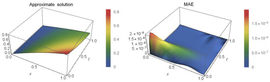
Figure 1 shows the approximate solution and the maximum absolute error ($MAE$) graphs for the case $N=12$ and $\ell =\tau =1$. This figure shows that the numerical solution is close to the exact solution. In Table 1, we illustrate the absolute error (AE) for different values of t at $N=12$ and $\ell =\tau =1$. This table fully shows that the expressed method has a good precision. Furthermore, the AEs for different values of t at $N=8$ when $\ell =3$ and $\tau =2$ are shown in Table 2. We can see from Table 1 and Table 2 and Figure 1 that the proposed method is appropriate and effective.

Figure 1. The approximate solution and the $MAE$ graphs of Example 1.

Table 1. The AEs of Example 1.

x	$\mathit{t}=\frac{2}{10}$	$\mathit{t}=\frac{4}{10}$	$\mathit{t}=\frac{6}{10}$	$\mathit{t}=\frac{8}{10}$
0.1	$1.07216\times {10}^{-6}$	$1.04375\times {10}^{-7}$	$1.04421\times {10}^{-8}$	$1.74522\times {10}^{-9}$
0.2	$1.01956\times {10}^{-6}$	$1.66463\times {10}^{-7}$	$1.97095\times {10}^{-8}$	$2.84439\times {10}^{-9}$
0.3	$9.15588\times {10}^{-7}$	$2.09069\times {10}^{-7}$	$2.70454\times {10}^{-8}$	$3.78237\times {10}^{-9}$
0.4	$7.82278\times {10}^{-7}$	$2.30326\times {10}^{-7}$	$3.17442\times {10}^{-8}$	$4.40703\times {10}^{-9}$
0.5	$6.37195\times {10}^{-7}$	$2.30262\times {10}^{-7}$	$3.33491\times {10}^{-8}$	$4.62481\times {10}^{-9}$
0.6	$4.92708\times {10}^{-7}$	$2.10443\times {10}^{-7}$	$3.17013\times {10}^{-8}$	$4.39902\times {10}^{-9}$
0.7	$3.55998\times {10}^{-7}$	$1.73636\times {10}^{-7}$	$2.69589\times {10}^{-8}$	$3.74448\times {10}^{-9}$
0.8	$2.29584\times {10}^{-7}$	$1.23449\times {10}^{-7}$	$1.95837\times {10}^{-8}$	$2.72157\times {10}^{-9}$
0.9	$1.12214\times {10}^{-7}$	$6.4063\times {10}^{-7}$	$1.02952\times {10}^{-8}$	$1.42996\times {10}^{-9}$

Table 2. The AEs of Example 1.

x	$\mathit{t}=\frac{3}{10}$	$\mathit{t}=\frac{7}{10}$	$\mathit{t}=\frac{11}{10}$	$\mathit{t}=\frac{15}{10}$	$\mathit{t}=\frac{19}{10}$
0.2	9.81704$\times {10}^{-5}$	2.42225$\times {10}^{-4}$	2.24868$\times {10}^{-6}$	5.37087$\times {10}^{-3}$	3.24886$\times {10}^{-3}$
0.4	1.61729$\times {10}^{-4}$	5.11161$\times {10}^{-4}$	4.67631$\times {10}^{-4}$	2.53555$\times {10}^{-3}$	1.11043$\times {10}^{-3}$
0.6	1.84251$\times {10}^{-4}$	8.30112$\times {10}^{-4}$	8.43864$\times {10}^{-4}$	8.92868$\times {10}^{-4}$	1.84493$\times {10}^{-3}$
0.8	1.26461$\times {10}^{-4}$	1.21323$\times {10}^{-3}$	1.14871$\times {10}^{-3}$	1.94866$\times {10}^{-4}$	4.31002$\times {10}^{-3}$
1	6.98793$\times {10}^{-5}$	1.66147$\times {10}^{-3}$	1.38598$\times {10}^{-3}$	2.11464$\times {10}^{-4}$	1.64701$\times {10}^{-3}$
1.2	4.82847$\times {10}^{-4}$	2.15759$\times {10}^{-3}$	1.54812$\times {10}^{-3}$	7.01591$\times {10}^{-4}$	3.46544$\times {10}^{-2}$
1.4	1.19936$\times {10}^{-3}$	2.66197$\times {10}^{-3}$	1.62211$\times {10}^{-3}$	1.39606$\times {10}^{-3}$	5.36674$\times {10}^{-2}$
1.6	2.29473$\times {10}^{-3}$	3.11052$\times {10}^{-3}$	1.59488$\times {10}^{-3}$	1.99516$\times {10}^{-3}$	6.71459$\times {10}^{-2}$
1.8	3.79811$\times {10}^{-3}$	3.41681$\times {10}^{-3}$	1.45906$\times {10}^{-3}$	2.18735$\times {10}^{-3}$	6.83315$\times {10}^{-2}$
2	5.64132$\times {10}^{-3}$	3.48161$\times {10}^{-3}$	1.21885$\times {10}^{-3}$	1.69924$\times {10}^{-3}$	5.15014$\times {10}^{-3}$
2.2	7.58846$\times {10}^{-3}$	3.21358$\times {10}^{-3}$	8.95812$\times {10}^{-4}$	3.90051$\times {10}^{-4}$	1.43644$\times {10}^{-2}$
2.4	9.14396$\times {10}^{-3}$	2.56621$\times {10}^{-3}$	5.33517$\times {10}^{-4}$	1.59222$\times {10}^{-3}$	3.82048$\times {10}^{-2}$
2.6	9.43725$\times {10}^{-3}$	1.59666$\times {10}^{-3}$	2.00103$\times {10}^{-4}$	3.57282$\times {10}^{-3}$	8.86543$\times {10}^{-2}$
2.8	7.08014$\times {10}^{-3}$	5.53469$\times {10}^{-4}$	1.32394$\times {10}^{-5}$	4.00638$\times {10}^{-3}$	9.89625$\times {10}^{-2}$

Example 2.

Consider the following heat conduction equation [47,48]:

$$\frac{\partial u(x,t)}{\partial t}-\frac{{\partial }^{2}u(x,t)}{\partial x^2}=0,0\le x\le \ell ,0\le t\le \tau ,$$

along with the following initial and boundary conditions:

$$\begin{array}{cc}\hfill & u(x,0)=e^{-\frac{x}{\sqrt{2}}}\cos \left(\frac{x}{\sqrt{2}}\right),\hfill \\ & u(0,t)=\cos \left(t\right),u(\ell ,t)=e^{-\frac{\ell }{\sqrt{2}}}\cos \left(t-\frac{\ell }{\sqrt{2}}\right),\hfill \end{array}$$

where the exact solution is: $u(x,t)=e^{-\frac{x}{\sqrt{2}}}\cos (t-\frac{x}{\sqrt{2}})$.

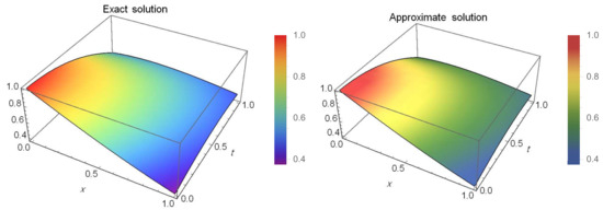
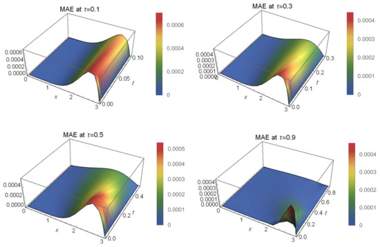
In Figure 2, we sketched the exact and approximate solutions for the case $N=12$ and $\ell =\tau =1.$ This figure shows that the numerical and exact solutions are almost identical. In Figure 3, we plotted the $MAE$s when $\ell =3$ and for different values of τ at $N=12.$ In Table 3, we list the $MAE$s for different values of N and for $\ell =\tau =1$. In Table 4, we give a comparison between the $MAE$s obtained from the application of the numerical scheme presented in [47] and our method. The results of Table 3 and Table 4 and Figure 2 and Figure 3 show that our numerical results when taking few terms of the proposed shifted fifth-kind Chebyshev expansion are more accurate. This demonstrates the advantage of our method when compared with some other numerical methods.

Figure 2. The exact and approximate solutions of Example 2.

Figure 3. $MAE$ graphs of Example 2.

Table 3. $MAE$s of Example 2.

N	2	4	6	8	10	12
$MAE$	$3.73882\times {10}^{-1}$	$1.57463\times {10}^{-2}$	$1.50513\times {10}^{-2}$	$3.26227\times {10}^{-3}$	$1.16386\times {10}^{-3}$	$1.30992\times {10}^{-8}$

Table 4. Comparison between our method and the method in [47] for Example 2.

Our method	$1.30992\times {10}^{-8}$
method in [47]	$2.28\times {10}^{-5}$

Example 3.

Consider the following heat conduction equation

$$\frac{\partial u(x,t)}{\partial t}-\frac{{\partial }^{2}u(x,t)}{\partial x^2}=-\frac{{(t+1)}^2{e}^x}{{\left(t^2+1\right)}^2},0\le x\le \ell ,0\le t\le \tau ,$$

along with the following initial and boundary conditions:

$$\begin{array}{cc}\hfill & u(x,0)=e^x,\hfill \\ & u(0,t)=\frac{1}{t^2+1},u(\ell ,t)=\frac{e^{\ell }}{t^2+1},\hfill \end{array}$$

where the exact solution is: $u(x,t)=\frac{e^x}{t^2+1}$.

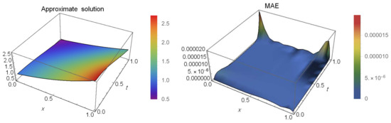
In Figure 4, we illustrate the approximate solution and the $MAE$ graphs for the case $N=12$ and $\ell =\tau =1$. Table 5 shows the AEs for different values of t at $N=12$ and $\ell =\tau =1$. This table fully reveals that the expressed method has a good precision. In Table 6, we report the AEs for different values of t at $N=10$ when $\ell =3$ and $\tau =1.$ We can see from the tabulated AEs of Table 5 and Table 6 and Figure 4 that the proposed method is suitable and powerful for solving the heat conduction equation.

Figure 4. The approximate solution and the $MAE$ graphs of Example 3.

Table 5. The AEs of Example 3.

x	$\mathit{t}=\frac{1}{10}$	$\mathit{t}=\frac{3}{10}$	$\mathit{t}=\frac{5}{10}$	$\mathit{t}=\frac{7}{10}$	$\mathit{t}=\frac{9}{10}$
0.1	$2.53661\times {10}^{-6}$	$6.78466\times {10}^{-7}$	$4.66726\times {10}^{-8}$	$6.34649\times {10}^{-9}$	$1.09628\times {10}^{-7}$
0.2	$2.12895\times {10}^{-6}$	$8.21776\times {10}^{-7}$	$9.03818\times {10}^{-8}$	$1.21842\times {10}^{-8}$	$2.68961\times {10}^{-9}$
0.3	$1.75779\times {10}^{-6}$	$8.88757\times {10}^{-7}$	$1.24666\times {10}^{-7}$	$1.69281\times {10}^{-8}$	$1.93979\times {10}^{-8}$
0.4	$1.43444\times {10}^{-6}$	$8.86624\times {10}^{-7}$	$1.46208\times {10}^{-7}$	$2.00541\times {10}^{-8}$	$5.19067\times {10}^{-9}$
0.5	$1.15321\times {10}^{-6}$	$8.25147\times {10}^{-7}$	$1.53111\times {10}^{-7}$	$2.11703\times {10}^{-8}$	$1.08241\times {10}^{-8}$
0.6	$9.01903\times {10}^{-7}$	$7.15177\times {10}^{-7}$	$1.44973\times {10}^{-7}$	$2.01492\times {10}^{-8}$	$2.08671\times {10}^{-8}$
0.7	$6.69298\times {10}^{-7}$	$5.67622\times {10}^{-7}$	$1.22826\times {10}^{-7}$	$1.71658\times {10}^{-8}$	$3.45005\times {10}^{-8}$
0.8	$4.45284\times {10}^{-7}$	$3.92877\times {10}^{-7}$	$8.89726\times {10}^{-8}$	$1.25433\times {10}^{-8}$	$4.42532\times {10}^{-9}$
0.9	$2.25786\times {10}^{-7}$	$3.92877\times {10}^{-7}$	$4.67338\times {10}^{-8}$	$6.77284\times {10}^{-9}$	$1.53647\times {10}^{-7}$

Table 6. The AEs of Example 3.

x	$\mathit{t}=\frac{1}{10}$	$\mathit{t}=\frac{4}{10}$	$\mathit{t}=\frac{7}{10}$	$\mathit{t}=1$
0	$1.75063\times {10}^{-7}$	$4.24278\times {10}^{-7}$	$2.88407\times {10}^{-8}$	$7.33871\times {10}^{-5}$
0.3	$2.16085\times {10}^{-5}$	$1.95217\times {10}^{-4}$	$2.59148\times {10}^{-4}$	$2.84798\times {10}^{-4}$
0.6	$7.64342\times {10}^{-5}$	$4.37391\times {10}^{-4}$	$5.12969\times {10}^{-4}$	$5.05394\times {10}^{-4}$
0.9	$2.26323\times {10}^{-4}$	$7.54558\times {10}^{-4}$	$7.48026\times {10}^{-4}$	$7.13391\times {10}^{-4}$
1.2	$5.74283\times {10}^{-4}$	$1.13808\times {10}^{-3}$	$9.39723\times {10}^{-4}$	$8.97356\times {10}^{-4}$
1.5	$1.24217\times {10}^{-3}$	$1.51991\times {10}^{-3}$	$1.05868\times {10}^{-4}$	$1.05103\times {10}^{-3}$
1.8	$2.28929\times {10}^{-3}$	$1.76226\times {10}^{-3}$	$1.08712\times {10}^{-3}$	$1.16802\times {10}^{-3}$
2.1	$3.55861\times {10}^{-3}$	$1.68673\times {10}^{-3}$	$1.03616\times {10}^{-3}$	$1.23095\times {10}^{-3}$
2.4	$4.47518\times {10}^{-3}$	$1.17726\times {10}^{-3}$	$9.38583\times {10}^{-4}$	$1.19524\times {10}^{-3}$
2.7	$3.87464\times {10}^{-3}$	$3.82554\times {10}^{-3}$	$7.46487\times {10}^{-4}$	$9.78603\times {10}^{-4}$
3	$5.70265\times {10}^{-7}$	$8.39831\times {10}^{-8}$	$2.23171\times {10}^{-7}$	$4.82824\times {10}^{-4}$

6. Concluding Remarks

In this paper, we treated numerically one of the well-known equations named the heat conduction equation. The shifted Chebyshev polynomials of the fifth kind were used as basis functions. Some new theoretical results concerning specific formulas of the derivatives and integrals formulas of these polynomials were established. A numerical scheme to solve this equation was analyzed and implemented in detail. The basic idea behind the proposed algorithm was built on solving the corresponding integral equation to the heat conduction equation, and after that employing the spectral tau method to convert the integral equation governed by its boundary condition into an algebraic system of equations that could be solved via a suitable numerical solver. The performance of our presented method was evaluated in terms of absolute errors and maximum absolute errors. The numerical results demonstrated the good accuracy of this scheme and the ability to simulate the exact solution well. All codes were written and debugged by Mathematica 11 on HP Z420 Workstation, Processor: Intel (R) Xeon(R) CPU E5-1620—3.6 GHz, 16 GB Ram DDR3, and 512 GB storage.

References

- Fourier, J. The Analytical Theory of Heat; The University Press: Oxford, UK, 1878. [Google Scholar]
- Narasimhan, T.N. Fourier’s heat conduction equation: History, influence, and connections. Rev. Geophys. 1999, 37, 151–172. [Google Scholar]
- Meyu, G.; Koriche, K. Analytical solution vs. numerical solution of heat equation flow through rod of length 8 units in one dimension. Int. J. Appl. Math. Theor. Phys. 2021, 7, 53. [Google Scholar] [CrossRef]
- Liu, C.S.; Chang, J.R. Solving a nonlinear heat equation with nonlocal boundary conditions by a method of nonlocal boundary shape functions. Numer. Heat Transf. Part B Fundam. 2021, 80, 1–13. [Google Scholar]
- Tassaddiq, A.; Yaseen, M.; Yousaf, A.; Srivastava, R. A cubic B-spline collocation method with new approximation for the numerical treatment of the heat equation with classical and non-classical boundary conditions. Phys. Scr. 2021, 96, 045212. [Google Scholar] [CrossRef]
- Dehghan, M.; Shirilord, A. The use of homotopy analysis method for solving generalized Sylvester matrix equation with applications. Eng. Comput. 2021, 38, 2699–2716. [Google Scholar] [CrossRef]
- Saratha, S.R.; Krishnan, G.S.S.; Bagyalakshmi, M. Analysis of a fractional epidemic model by fractional generalised homotopy analysis method using modified Riemann-Liouville derivative. Appl. Math. Model. 2021, 92, 525–545. [Google Scholar] [CrossRef]
- Gonzalez-Gaxiola, O.; Biswas, A.; Ekici, M.; Khan, S. Highly dispersive optical solitons with quadratic–cubic law of refractive index by the variational iteration method. J. Opt. 2021, 51, 29–36. [Google Scholar] [CrossRef]
- Doeva, O.; Masjedi, P.K.; Weaver, P.M. A semi-analytical approach based on the variational iteration method for static analysis of composite beams. Compos. Struct. 2021, 257, 113110. [Google Scholar]
- Noeiaghdam, S.; Sidorov, D.; Wazwaz, A.M.; Sidorov, N.; Sizikov, V. The Numerical Validation of the Adomian Decomposition Method for Solving Volterra Integral Equation with Discontinuous Kernels Using the CESTAC Method. Mathematics 2021, 9, 260. [Google Scholar] [CrossRef]
- Lu, T.T.; Zheng, W.Q. Adomian decomposition method for first order PDEs with unprescribed data. Alex. Eng. J. 2021, 60, 2563–2572. [Google Scholar]
- Li, P.W. Space–time generalized finite difference nonlinear model for solving unsteady Burgers’ equations. Appl. Math. Lett. 2021, 114, 106896. [Google Scholar]
- Bullo, T.; Duressa, G.F.; Degla, G. Accelerated fitted operator finite difference method for singularly perturbed parabolic reaction-diffusion problems. Comput. Meth. Diff. Eqs. 2021, 9, 886–898. [Google Scholar]
- Vargas, A.M. Finite difference method for solving fractional differential equations at irregular meshes. Math. Comput. Simul. 2022, 193, 204–216. [Google Scholar] [CrossRef]
- Gharibi, Z.; Dehghan, M. Convergence analysis of weak Galerkin flux-based mixed finite element method for solving singularly perturbed convection-diffusion-reaction problem. Appl. Numer. Math. 2021, 163, 303–316. [Google Scholar]
- Yu, B.; Hu, P.; Saputra, A.A.; Gu, Y. The scaled boundary finite element method based on the hybrid quadtree mesh for solving transient heat conduction problems. Appl. Math. Model. 2021, 89, 541–571. [Google Scholar] [CrossRef]
- Namala, S.; Uddin, R. Hybrid nodal integral/finite element method for time-dependent convection diffusion equation. J. Nuc. Eng. Radiat. Sci. 2022, 8, 021406. [Google Scholar] [CrossRef]
- Zhang, H.; Liu, F.; Jiang, X.; Turner, I. Spectral method for the two-dimensional time distributed-order diffusion-wave equation on a semi-infinite domain. J. Comput. Appl. Math. 2022, 399, 113712. [Google Scholar]
- Atta, A.G.; Moatimid, G.M.; Youssri, Y.H. Generalized Fibonacci Operational tau Algorithm for Fractional Bagley-Torvik Equation. Prog. Fract. Differ. Appl. 2020, 6, 215–224. [Google Scholar]
- Tu, H.; Wang, Y.; Lan, Q.; Liu, W.; Xiao, W.; Ma, S. A Chebyshev-Tau spectral method for normal modes of underwater sound propagation with a layered marine environment. J. Sound Vib. 2021, 492, 115784. [Google Scholar] [CrossRef]
- Doha, E.H.; Abd-Elhameed, W.M. Accurate spectral solutions for the parabolic and elliptic partial differential equations by the ultraspherical tau method. J. Comput. Appl. Math. 2005, 181, 24–45. [Google Scholar] [CrossRef]
- Atta, A.G.; Moatimid, G.M.; Youssri, Y.H. Generalized Fibonacci operational collocation approach for fractional initial value problems. Int. J. Appl. Comput. Math. 2019, 5, 1–11. [Google Scholar] [CrossRef]
- Hesthaven, J.S.; Gottlieb, S.; Gottlieb, D. Spectral Methods for Time-Dependent Problems; Cambridge University Press: Cambridge, UK, 2007; Volume 21. [Google Scholar]
- Shizgal, B. Spectral Methods in Chemistry and Physics; Springer: Berlin/Heidelberg, Germany, 2015. [Google Scholar]
- Costabile, F.; Napoli, A. A class of Birkhoff–Lagrange-collocation methods for high order boundary value problems. Appl. Numer. Math. 2017, 116, 129–140. [Google Scholar]
- Youssri, Y.H. Orthonormal Ultraspherical Operational Matrix Algorithm for Fractal–Fractional Riccati Equation with Generalized Caputo Derivative. Fractal Fract. 2021, 5, 100. [Google Scholar]
- Abd-Elhameed, W.M.; Youssri, Y.H. Explicit shifted second-kind Chebyshev spectral treatment for fractional Riccati differential equation. CMES Comput. Model. Eng. Sci. 2019, 121, 1029–1049. [Google Scholar]
- Atta, A.G.; Abd-Elhameed, W.M.; Moatimid, G.M.; Youssri, Y.H. Shifted fifth-kind Chebyshev Galerkin treatment for linear hyperbolic first-order partial differential equations. Appl. Numer. Math. 2021, 167, 237–256. [Google Scholar]
- Atta, A.G.; Abd-Elhameed, W.M.; Youssri, Y.H. Shifted fifth-kind Chebyshev polynomials Galerkin-based procedure for treating fractional diffusion-wave equation. Int. J. Mod. Phys. C 2022, 33, 2250102. [Google Scholar] [CrossRef]
- Khalil, H.; Khan, R.A. A new method based on Legendre polynomials for solutions of the fractional two-dimensional heat conduction equation. Comput. Math. Appl. 2014, 67, 1938–1953. [Google Scholar]
- Abbasbandy, S.; Kazem, S.; Alhuthali, M.S.; Alsulami, H.H. Application of the operational matrix of fractional-order Legendre functions for solving the time-fractional convection–diffusion equation. Appl. Math. Comput. 2015, 266, 31–40. [Google Scholar] [CrossRef]
- Abdelkawy, M.A.; Alyami, S.A. Legendre-Chebyshev spectral collocation method for two-dimensional nonlinear reaction-diffusion equation with Riesz space-fractional. Chaos Solitons Fractals 2021, 151, 111279. [Google Scholar]
- Atta, A.G.; Abd-Elhameed, W.M.; Moatimid, G.M.; Youssri, Y.H. Advanced shifted sixth-kind Chebyshev tau approach for solving linear one-dimensional hyperbolic telegraph type problem. Math. Sci. 2022. [Google Scholar] [CrossRef]
- Pourbabaee, M.; Saadatmandi, A. Collocation method based on Chebyshev polynomials for solving distributed order fractional differential equations. Comput. Meth. Differ. Eqs. 2021, 9, 858–873. [Google Scholar]
- Mohammadi, F.; Moradi, L.; Conte, D. Discrete Chebyshev polynomials for solving fractional variational problems. Stat. Optim. Inf. Comput. 2021, 9, 502–515. [Google Scholar] [CrossRef]
- Abbas, W.; Fathy, M.; Mostafa, M.; Hashem, A.M.A. Galerkin method for nonlinear Volterra-Fredholm integro-differential equations based on Chebyshev polynomials. Eng. Res. J. 2021, 170, 169–183. [Google Scholar]
- Panghal, S.; Kumar, M. Multilayer perceptron and Chebyshev polynomials-based functional link artificial neural network for solving differential equations. Int. J. Model. Simulat. Sci. Comput. 2021, 12, 2150011. [Google Scholar] [CrossRef]
- Abd-Elhameed, W.M. Novel expressions for the derivatives of sixth kind Chebyshev polynomials: Spectral solution of the non-linear one-dimensional Burgers’ Equation. Fractal Fract. 2021, 5, 53. [Google Scholar] [CrossRef]
- Doha, E.H.; Abd-Elhameed, W.M.; Bassuony, M.A. On the coefficients of differentiated expansions and derivatives of Chebyshev polynomials of the third and fourth kinds. Acta Math. Sci. 2015, 35, 326–338. [Google Scholar] [CrossRef]
- Doha, E.H.; Abd-Elhameed, W.M.; Bassuony, M.A. On using third and fourth kinds Chebyshev operational matrices for solving Lane-Emden type equations. Rom. J. Phys. 2015, 60, 281–292. [Google Scholar]
- Sadri, K.; Aminikhah, H. A new efficient algorithm based on fifth-kind Chebyshev polynomials for solving multi-term variable-order time-fractional diffusion-wave equation. Int. J. Comput. Math. 2021, 99, 966–992. [Google Scholar] [CrossRef]
- Abd-Elhameed, W.M.; Youssri, Y.H. New formulas of the high-order derivatives of fifth-kind Chebyshev polynomials: Spectral solution of the convection–diffusion equation. Numer. Methods Partial. Differ. Equ. 2021. [Google Scholar] [CrossRef]
- Abd-Elhameed, W.M.; Youssri, Y.H. Fifth-kind orthonormal Chebyshev polynomial solutions for fractional differential equations. Comput. Appl. Math. 2018, 37, 2897–2921. [Google Scholar] [CrossRef]
- Koepf, W. Hypergeometric Summation, 2nd ed.; Springer Universitext Series: Berlin/Heidelberg, Germany, 2014. [Google Scholar]
- Li, J.; Cheng, Y. Linear barycentric rational collocation method for solving heat conduction equation. Numer. Methods Partial. Differ. Equ. 2021, 37, 533–545. [Google Scholar] [CrossRef]
- Merga, F.E.; Chemeda, H.M. Modified Crank-Nicolson scheme with Richardson extrapolation for one-dimensional heat equation. Iran. J. Sci. Technol. Trans. Sci. 2021, 45, 1725–1734. [Google Scholar] [CrossRef]
- Hamaidi, M.; Naji, A.; Charafi, A. Space–time localized radial basis function collocation method for solving parabolic and hyperbolic equations. Eng. Anal. Bound. Elem. 2016, 67, 152–163. [Google Scholar] [CrossRef]
- Ku, C.Y.; Liu, C.Y.; Xiao, J.E.; Chen, M.R. Solving backward heat conduction problems using a novel space–time radial polynomial basis function collocation method. Appl. Sci. 2020, 10, 3215. [Google Scholar]
Publisher’s Note: MDPI stays neutral with regard to jurisdictional claims in published maps and institutional affiliations. |
© 2022 by the authors. Licensee MDPI, Basel, Switzerland. This article is an open access article distributed under the terms and conditions of the Creative Commons Attribution (CC BY) license (https://creativecommons.org/licenses/by/4.0/).