Stability of a Nonlinear Langevin System of ML-Type Fractional Derivative Affected by Time-Varying Delays and Differential Feedback Control

Abstract

The Langevin system is an important mathematical model to describe Brownian motion. The research shows that fractional differential equations have more advantages in viscoelasticity. The exploration of fractional Langevin system dynamics is novel and valuable. Compared with the fractional system of Caputo or Riemann–Liouville (RL) derivatives, the system with Mittag–Leffler (ML)-type fractional derivatives can eliminate singularity such that the solution of the system has better analytical properties. Therefore, we concentrate on a nonlinear Langevin system of ML-type fractional derivatives affected by time-varying delays and differential feedback control in the manuscript. We first utilize two fixed-point theorems proposed by Krasnoselskii and Schauder to investigate the existence of a solution. Next, we employ the contraction mapping principle and nonlinear analysis to establish the stability of types such as Ulam–Hyers (UH) and Ulam–Hyers–Rassias (UHR) as well as generalized UH and UHR. Lastly, the theoretical analysis and numerical simulation of some interesting examples are carried out by using our main results and the DDESD toolbox of MATLAB.

1. Introduction

This work mostly takes into account a nonlinear Langevin system of ML-type fractional derivatives affected by time-varying delays and differential feedback control as follows:

$$\begin{array}{c}\hfill \left\{\begin{array}{c}{}^{ML}{\mathcal{D}}_{0^{+}}^{\beta }\left[{}^{ML}{\mathcal{D}}_{0^{+}}^{\alpha }-\lambda \right]u\left(t\right)=f(t,u(t-{\sigma }_1\left(t\right)),w(t-{\sigma }_2\left(t\right))),t\in (0,b],\hfill \\ w^{\prime }\left(t\right)=g(t,u(t-{\sigma }_3\left(t\right)),w(t-{\sigma }_4\left(t\right))),t\in J=[0,b],\hfill \\ u\left(t\right)={\omega }_1\left(t\right),w\left(t\right)={\omega }_2\left(t\right),{}^{ML}{\mathcal{D}}_{0^{+}}^{\alpha }u\left(t\right)={\omega }_3\left(t\right),t\in [-\sigma ,0],\hfill \end{array}\right.\end{array}$$

(1)

where $0<\alpha ,\beta \le 1$ and $b,\lambda >0$, ${}^{ML}{\mathcal{D}}_{0^{+}}^{\kappa }$ is the ML-type fractional derivative with $\kappa$-order, for all $0<\kappa \le 1$. $f,g\in C(J\times {\mathbb{R}}^2,\mathbb{R})$, ${\sigma }_l\in C(J,{\mathbb{R}}^{+})(l=1,2,3,4)$, $\sigma ={max}_{1\le l\le 4}\left\{{max}_{t\in J}{\sigma }_l\left(t\right)\right\}$, ${\omega }_m\in C([-\sigma ,0],\mathbb{R})(m=1,2,3)$.

The main motivation comes from the important theory and wide application of the Langevin system. In 1908, the French physicist Paul Langevin put forward the famous Langevin equation to expound the random motion of particles annihilated in the fluid due to the collision between particles and fluid molecules. In [1,2], the authors provided a large number of random examples of the Langevin system as mathematical models. The fractional-order Langevin system makes up for the deficiency of the integer-order Langevin system and has been widely used and studied. The integer-order Langevin system can not meet the accuracy requirements in describing complex viscoelasticity. Therefore, the classical Langevin system has been extended and modified. For example, Kubo [3,4] imitated a complex viscoelastic abnormal diffusion process by applying a general Langevin system. It is worth noting that the derivatives in these generalized equations are of integer order. Because fractional derivatives have advantages in describing the process of memory and viscoelasticity, another modification is to replace the integral derivative with a fractional derivative in the Langevin system. The early research on the fractional Langevin system as a model was conducted by Eab and Lim [5] as well as Sandev and Tomovski [6]. They used the fractional Langevin system to study the one-dimensional diffusion process and the motion of free particles driven by power law noise, respectively. Recently, some new fields have emerged in the application of fractional differential systems (see [7,8,9,10]). Additionally, some important achievements have been made in the research of the fractional Langevin system (see [11,12,13,14,15,16,17]).

Furthermore, for a system with practical application background, its stability is very important. According to practical needs, scientists have put forward many concepts of system stability. UH-stability is one of the most important stabilities, which was posed by Ulam and Hyers [18,19] in the 1940s. In the last ten years, the research on the UH-stability of fractional systems has been highly praised by many scholars. There have many papers dealing with the UH-stability [20,21,22,23,24,25,26] and generalized UH-stability [27,28,29] of fractional system. However, only a few papers [30,31,32,33,34] have discussed that the fractional Langevin system is UH-stable.

It is worth noting that the previous works on the fractional Langevin system basically involve Caputo- or RL-fractional derivatives. However, under certain circumstances, the singularity of Caputo or Riemann–Liouville fractional derivatives is unavoidable. This leads to huge errors and even distortion in the application of the Caputo or Riemann–Liouville fractional system in some physical fields. Hence, some scholars began to modify the previous definition of a fractional derivative to eliminate singularity. For instance, Caputo and Febrizio raised a nonsingular fractional derivative (see [35]), which is called the Caputo–Febrizio fractional derivative. In [36], Atangana and Baleanu proposed another novel nonsingular fractional derivative with an ML-kernel. In both theory [37,38,39,40] and application [41,42,43,44,45,46,47], many scholars have focused on the study of these nonsingular fractional systems since they were put forward. However, only rare published works [48,49] have shown that some ML-type fractional Langevin systems are UH-stable.

Inspired by the aforementioned, the main purpose of this manuscript is to find some sufficient conditions for the existence and stability of the solution of system (1). The main contributions of our work are reflected in the following aspects. (i) Comparison with previous works on fractional Langevin equation such as [30,31,32], our system (1) involves nonsingular fractional derivatives with an ML-kernel. (ii) In system (1), we consider the influence of delayed differential feedback control, which is not found in previous papers. (iii) We obtain some new criteria of existence and UH-type stability of solutions. (iv) By applying the DDESD toolbox of MATLAB, the simulations and numerical solutions are given.

In Section 2, we will review some concepts and lemmas used later. Based on some fixed-point theorems, we prove that system (1) has at least a solution in Section 3. The UH-, UHR-, GUH-, and GUHR-stability of (1) are built in Section 4. As applications, we conduct theoretical analysis and numerical simulation on some examples to verify the correctness and effectiveness of our main results in Section 5. Finally, a brief summary is made in Section 6. In addition, we put lengthy and complex theoretical proofs in the appendices to improve the readability and conciseness of the manuscript.

2. Preliminaries

Definition 1

([50]). Let $0<\alpha \le 1$, $b>0$, $u:[0,b]\to \mathbb{R}$. Define an integral

$$\begin{array}{c}\hfill {}^{ML}{\mathcal{I}}_{0^{+}}^{\alpha }u\left(t\right)=\frac{1-\alpha }{\mathcal{N}\left(\alpha \right)}u\left(t\right)+\frac{\alpha }{\mathcal{N}\left(\alpha \right)\Gamma \left(\alpha \right)}{\int }_0^t{(t-x)}^{\alpha -1}u\left(x\right)dx,\end{array}$$

where $\Gamma \left(\alpha \right)={\int }_0^{\infty }{x}^{\alpha -1}{e}^{-x}dx$, the normalized constant $\mathcal{N}\left(\alpha \right)$ satisfies $\mathcal{N}\left(0\right)=\mathcal{N}\left(1\right)=1$. If the above integral exists, then it is called the α-order ML-fractional integral along the left of u.

Definition 2

([36]). Let $0<\alpha \le 1$, $b>0$ and $u\in C^1(0,b)$. The α-order ML-fractional derivative along the left of u in sense of Caputo is defined by

$$\begin{array}{c}\hfill {}^{ML}{\mathcal{D}}_{0^{+}}^{\alpha }u\left(t\right)=\frac{\mathcal{N}\left(\alpha \right)}{(1-\alpha )}{\int }_0^t{\mathbb{E}}_{\alpha }\left[-\frac{\alpha }{1-\alpha }{(t-x)}^{\alpha }\right]u^{\prime }\left(x\right)dx,\end{array}$$

where ${\mathbb{E}}_{\alpha }\left(z\right)={\sum }_{k=0}^{\infty }\frac{z^k}{\Gamma (\alpha k+1)}$ is is called the one-parameter ML-function.

Lemma 1

([37]). Given $0<\nu \le 1$ and $h\in C[0,b]$, then the following ML-fractional system

$$\begin{array}{c}\hfill \left\{\begin{array}{c}{}^{ML}{\mathcal{D}}_{0^{+}}^{\nu }w\left(t\right)=h\left(t\right),t\in (0,b),\hfill \\ w\left(0\right)=w_0,\hfill \end{array}\right.\end{array}$$

is uniquely solved by

$$\begin{array}{c}\hfill w\left(t\right)=w_0+\frac{1-\nu }{\mathcal{N}\left(\nu \right)}[h\left(t\right)-h\left(0\right)]+\frac{\nu }{\mathcal{N}\left(\nu \right)\Gamma \left(\nu \right)}{\int }_0^t{(t-x)}^{\nu -1}h\left(x\right)dx.\end{array}$$

Remark 1.

Definition 2 and Lemma 1 imply that ${}^{ML}{\mathcal{D}}_{0^{+}}^{\alpha }u\left(t\right)\equiv 0$ iff $u\left(t\right)$ is identical to a constant.

The whole paper needs the following fundamental assumptions.

$\left({\mathrm{A}}_1\right)$

$\lambda ,b>0$ and $0<\alpha ,\beta \le 1$ are given constants such that $\Delta \triangleq 1-\frac{\lambda (1-\alpha )}{\mathcal{N}\left(\alpha \right)}\ne 0$.

$\left({\mathrm{A}}_2\right)$

$f,g\in C(J\times {\mathbb{R}}^2,\mathbb{R})$, ${\sigma }_l\in C(J,{\mathbb{R}}^{+})(l=1,2,3,4)$, $\sigma ={max}_{1\le l\le 4}\left\{{max}_{t\in J}{\sigma }_l\left(t\right)\right\}$, ${\omega }_m\in C([-\sigma ,0],\mathbb{R})(m=1,2,3)$.

Consider the below nonlinear integral system

$$\begin{array}{c}\hfill \left\{\begin{array}{c}u\left(t\right)={\omega }_1\left(0\right)+\frac{1}{\Delta }\{\frac{{\omega }_3\left(0\right)-\lambda {\omega }_1\left(0\right)}{\mathcal{N}\left(\alpha \right)\Gamma \left(\alpha \right)}{t}^{\alpha }-\frac{(1-\alpha )(1-\beta )}{\mathcal{N}\left(\alpha \right)\mathcal{N}\left(\beta \right)}f(0,{\omega }_1(-{\sigma }_1\left(0\right)),\omega (-{\sigma }_2\left(0\right)))\hfill \\ +\frac{(1-\alpha )(1-\beta )}{\mathcal{N}\left(\alpha \right)\mathcal{N}\left(\beta \right)}f(t,u(t-{\sigma }_1\left(t\right)),w(t-{\sigma }_2\left(t\right)))+\frac{\lambda \alpha }{\mathcal{N}\left(\alpha \right)\Gamma \left(\alpha \right)}{\int }_0^t{(t-s)}^{\alpha -1}u\left(s\right)ds\hfill \\ +\frac{(1-\alpha )\beta }{\mathcal{N}\left(\alpha \right)\mathcal{N}\left(\beta \right)\Gamma \left(\beta \right)}{\int }_0^t{(t-s)}^{\beta -1}f(s,u(s-{\sigma }_1\left(s\right)),w(s-{\sigma }_2\left(s\right)))ds\hfill \\ +\frac{\alpha (1-\beta )}{\mathcal{N}\left(\alpha \right)\mathcal{N}\left(\beta \right)\Gamma \left(\alpha \right)}{\int }_0^t{(t-s)}^{\alpha -1}f(s,u(s-{\sigma }_1\left(s\right)),w(s-{\sigma }_2\left(s\right)))ds\hfill \\ +\frac{\alpha \beta }{\mathcal{N}\left(\alpha \right)\mathcal{N}\left(\beta \right)\Gamma (\alpha +\beta )}{\int }_0^t{(t-s)}^{\alpha +\beta -1}f(s,u(s-{\sigma }_1\left(s\right)),w(s-{\sigma }_2\left(s\right)))ds\},t\in J,\hfill \\ w\left(t\right)={\omega }_2\left(0\right)+{\int }_0^{t}g(s,u(s-{\sigma }_3\left(s\right)),w(s-{\sigma }_4\left(s\right)))ds,t\in J,\hfill \\ u\left(t\right)={\omega }_1\left(t\right),w\left(t\right)={\omega }_2\left(t\right),t\in [-\sigma ,0].\hfill \end{array}\right.\end{array}$$

(2)

Lemma 2.

If conditions $\left({\mathrm{A}}_1\right)$ and $\left({\mathrm{A}}_2\right)$ are true, then, solving the nonlinear ML-fractional system (1) and solving the nonlinear integral system (2) are equivalent.

Remark 2.

Lemma 2 is the foundation of studying the existence and stability of solutions to system (1). Its proof is shown in Appendix A.

3. Existence of Solutions

In this section, by applying the following important fixed-point theorems, we emphasize studying the existence of solutions for system (1).

Lemma 3

(Krasnoselskii’s fixed-point theorem [51]). Let $\mathbb{X}$ be a Banach space, and $\varphi \ne \mathbb{Y}\subset \mathbb{X}$ be closed convex. If the mappings $\mathcal{P},\mathcal{Q}:\mathbb{Y}\to \mathbb{Y}$ fulfill the following conditions:

$\left(\mathrm{i}\right)$

$\mathcal{P}u+\mathcal{Q}v\in \mathbb{Y}$, $\forall u,v\in \mathbb{Y}$.

$\left(\mathrm{ii}\right)$

$\mathcal{P}$ is contraction and $\mathcal{Q}$ is continuous and compact.

Then, there has at least a solution $u^{*}\in \mathbb{Y}$ such that $u^{*}=\mathcal{P}{u}^{*}+\mathcal{Q}{u}^{*}$.

Lemma 4

(Schauder’s fixed point theorem [52]). Given a Banach space $\mathbb{X}$, let $\Omega \subset \mathbb{X}$ be closed convex, and define a mapping $\mathcal{T}:\overline{\Omega }\to \overline{\Omega }$. Then, there is a $u^{*}\in \overline{\Omega }$ such that $\mathcal{T}{u}^{*}=u^{*}$, provided that $\mathcal{T}$ is completely continuous.

It is easy to see from (2) that the solution of (1) can only meet the continuity. So we define some Banach spaces $\mathbb{Y}=C(I,\mathbb{R})$ with the norm ${\parallel z\parallel }_C={max}_{t\in I}\left|z\left(t\right)\right|$, and $\mathbb{X}=\mathbb{Y}\times \mathbb{Y}$ equipped with the norm $\parallel U\parallel =max\{\parallel u{\parallel }_C,\parallel w{\parallel }_C\}$, where $I=[-\sigma ,T]$ and $U=(u,v)\in \mathbb{X}$. We shall study the existence and stability of the solution of (1) in $(\mathbb{X},\parallel ·\parallel )$.

Under the basic assumptions $\left({\mathrm{A}}_1\right)$ and $\left({\mathrm{A}}_2\right)$, we obtain the following two solvability results of system (1).

Theorem 1.

Assume that $\left({\mathrm{A}}_1\right)$ and $\left({\mathrm{A}}_2\right)$ hold. If conditions $\left({\mathrm{A}}_3\right)$ and $\left({\mathrm{A}}_4\right)$ are satisfied:

$\left({\mathrm{A}}_3\right)$

There exist some functions $m_1\left(t\right),m_2\left(t\right)\in C(J,{\mathbb{R}}^{+})$ such that

$$\begin{array}{c}\hfill \left|f(t,u,w)\right|\le m_1\left(t\right),\left|g(t,u,w)\right|\le m_2\left(t\right),\forall t\in J,u,w\in \mathbb{R};\end{array}$$

$\left({\mathrm{A}}_4\right)$

$0<\kappa \triangleq \frac{\lambda b^{\alpha }}{|\Delta |\mathcal{N}\left(\alpha \right)\Gamma \left(\alpha \right)}<1;$

then system (1) has at least one solution $(u^{*}\left(t\right),w^{*}\left(t\right))\in \mathbb{X}$.

Theorem 2.

Assume that $\left({\mathrm{A}}_1\right)$ and $\left({\mathrm{A}}_2\right)$ hold. If conditions $\left({\mathrm{A}}_5\right)$ and $\left({\mathrm{A}}_6\right)$ are satisfied:

$\left({\mathrm{A}}_5\right)$

There exist some functions $M_k\left(t\right),N_k\left(t\right)\in C(J,{\mathbb{R}}^{+})(k=1,2,3)$ such that, $\forall t\in J,u,w\in \mathbb{R}$,

$$\left|f(t,u,w)\right|\le M_1\left(t\right)+M_2\left(t\right)\left|u\right|+M_3\left(t\right)\left|w\right|,\left|g(t,u,w)\right|\le N_1\left(t\right)+N_2\left(t\right)\left|u\right|+N_3\left(t\right)\left|w\right|;$$

$\left({\mathrm{A}}_6\right)$

$0<{\Theta }_1,{\Theta }_2<1$, where ${\Theta }_1=\frac{\lambda b^{\alpha }}{|\Delta |\mathcal{N}\left(\alpha \right)\Gamma \left(\alpha \right)}+\frac{\parallel M_2{\parallel }_b+{\parallel M_3\parallel }_b}{|\Delta |\mathcal{N}\left(\alpha \right)\mathcal{N}\left(\beta \right)}\left[2(1-\alpha )(1-\beta )+\frac{(1-\alpha )b^{\beta }}{\Gamma \left(\beta \right)}+\frac{(1-\beta )b^{\alpha }}{\Gamma \left(\alpha \right)}+\frac{\alpha \beta b^{\alpha +\beta }}{\Gamma (\alpha +\beta +1)}\right]$, ${\Theta }_2=b\left(\parallel N_2{\parallel }_b+{\parallel N_3\parallel }_b\right)$, ${\parallel ·\parallel }_b={max}_{t\in [0,b]}|·|$ and ${\parallel ·\parallel }_{\sigma }={max}_{t\in [-\sigma ,0]}|·|;$

then system (1) has at least one solution $(u^{*}\left(t\right),w^{*}\left(t\right))\in \mathbb{X}$.

Remark 3.

We apply Lemma 3 to prove Theorem 1 in three steps. Step 1 is to define two appropriate mappings $\mathcal{P}$, $\mathcal{Q}:\mathbb{X}\to \mathbb{X}$ as

$$\begin{array}{c}\hfill \left(\mathcal{P}U\right)\left(t\right)=(\left({\mathcal{P}}_{1}U\right)\left(t\right),\left({\mathcal{P}}_{2}U\right)\left(t\right)),\left(\mathcal{Q}U\right)\left(t\right)=(\left({\mathcal{Q}}_{1}U\right)\left(t\right),\left({\mathcal{Q}}_{2}U\right)\left(t\right)).\end{array}$$

Step 2 is to prove that $\mathcal{P}$ is contraction. Step 3 is to show that $\mathcal{Q}$ is continuous and compact based on the Arzelá–Ascoli theorem. The detailed proof of Theorem 1 can be seen in Appendix B. Similarly, an appropriate mapping $\mathcal{T}:\mathbb{X}\to \mathbb{X}$ is defined by

$$\begin{array}{c}\hfill \left(\mathcal{T}U\right)\left(t\right)=(\left({\mathcal{T}}_{1}U\right)\left(t\right),\left({\mathcal{T}}_{2}U\right)\left(t\right)),\forall t\in I=[-\sigma ,T],U=(u,w)\in \mathbb{X},\end{array}$$

we also employ Schauder’s fixed-point theorem (i.e., Lemma 4) to give the concrete proof of Theorem 2 in the Appendix C.

Remark 4.

Theorem 1 and Theorem 2 do not imply each other. In fact, condition $\left({\mathrm{A}}_3\right)$ is true ⇒ condition $\left({\mathrm{A}}_5\right)$ is also true, otherwise, it may not be true. However, condition $\left(A_6\right)$ is true ⇒ condition $\left({\mathrm{A}}_4\right)$ is also true, otherwise, it may not be true.

4. Stability of Ulam–Hyers type Systems

This section mainly discusses the stability of types such as Ulam–Hyers (UH) and Ulam–Hyers–Rassias (UHR) as well as generalized UH and UHR for system (1).

Lemma 5.

[52] Given a Banach space $\mathbb{X}$, let $\varphi \ne \mathbb{E}\subset \mathbb{X}$ be closed, and define a mapping $\mathcal{T}:\mathbb{E}\to \mathbb{E}$. Assume that $\mathcal{T}$ is contractive, then, there has a unique $u^{*}\in \mathbb{E}$ such that $\mathcal{T}{u}^{*}=u^{*}$.

Consider two inequalities as follows:

$$\begin{array}{c}\hfill \left\{\begin{array}{c}|{}^{ML}{\mathcal{D}}_{0^{+}}^{\beta }\left[{}^{ML}{\mathcal{D}}_{0^{+}}^{\alpha }-\lambda \right]x\left(t\right)-f(t,x(t-{\sigma }_1\left(t\right)),y(t-{\sigma }_2\left(t\right)))|\le ϵ,0<t\le b,\hfill \\ |y^{\prime }\left(t\right)-g(t,x(t-{\sigma }_3\left(t\right)),y(t-{\sigma }_4\left(t\right)))|\le ϵ,0<t\le b,\hfill \\ x\left(t\right)={\omega }_1\left(t\right),y\left(t\right)={\omega }_2\left(t\right),{}^{ML}{\mathcal{D}}_{0^{+}}^{\alpha }x\left(t\right)={\omega }_3\left(t\right),t\in [-\sigma ,0],\hfill \end{array}\right.\end{array}$$

(3)

and

$$\begin{array}{c}\hfill \left\{\begin{array}{c}|{}^{ML}{\mathcal{D}}_{0^{+}}^{\beta }\left[{}^{ML}{\mathcal{D}}_{0^{+}}^{\alpha }-\lambda \right]x\left(t\right)-f(t,x(t-{\sigma }_1\left(t\right)),y(t-{\sigma }_2\left(t\right)))|\le \phi \left(t\right)ϵ,0<t\le b,\hfill \\ |y^{\prime }\left(t\right)-g(t,x(t-{\sigma }_3\left(t\right)),y(t-{\sigma }_4\left(t\right)))|\le \phi \left(t\right)ϵ,0<t\le b,\hfill \\ x\left(t\right)={\omega }_1\left(t\right),y\left(t\right)={\omega }_2\left(t\right),{}^{ML}{\mathcal{D}}_{0^{+}}^{\alpha }x\left(t\right)={\omega }_3\left(t\right),t\in [-\sigma ,0],\hfill \end{array}\right.\end{array}$$

(4)

where $ϵ>0$, $0<\alpha ,\beta \le 1$, and $\phi :[-\sigma ,b]\to {\mathbb{R}}^{+}$ is continuously non-decreasing.

Similar to [18,19], we define the UH-type stability corresponding to (1) as follows.

Definition 3.

Let $X=(x,y)$ and $U=(u,w)$ in $\mathbb{X}$ be any solution of inequality (3) and the unique solution of system (1). For each $ϵ>0$,

$\left(1\right)$

if there exists a constant $C_1>0$ such that

$$\begin{array}{c}\hfill \parallel X\left(t\right)-U\left(t\right)\parallel \le C_1ϵ,\end{array}$$

then system (1) is called UH-stable;

$\left(2\right)$

if there exists a continuous function $\theta :\mathbb{R}\to {\mathbb{R}}^{+}$ with $\theta \left(0\right)=0$ such that

$$\begin{array}{c}\hfill \parallel X\left(t\right)-U\left(t\right)\parallel \le \theta \left(ϵ\right),\end{array}$$

then system (1) is called generalized UH-stable.

Definition 4.

Let $X=(x,y)$ and $U=(u,w)$ in $\mathbb{X}$ be any solution of inequality (4) and the unique solution of system (1). For each $ϵ>0$,

$\left(1\right)$

if there exists a constant $C_2>0$ such that

$$\begin{array}{c}\hfill \parallel X\left(t\right)-U\left(t\right)\parallel \le C_2\phi \left(t\right)ϵ,t\in [-\sigma ,b],\end{array}$$

then system (1) is called UHR-stable;

$\left(2\right)$

if there exists a constant $C_3>0$ such that

$$\begin{array}{c}\hfill \parallel X\left(t\right)-U\left(t\right)\parallel \le C_3\phi \left(t\right),t\in [-\sigma ,b],\end{array}$$

then system (1) is called generalized UHR-stable.

Obviously, UH-stable ⇒ generalized UH-stable, and UHR-stable ⇒ generalized UHR-stable.

Remark 5.

A function $X=(x,y)\in \mathbb{X}$ solves the inequality (3) iff there has a continuous vector function $\varphi =({\varphi }_1,{\varphi }_2)$ in $(0,b]$ such that

$\left(1\right)$

$|{\varphi }_1\left(t\right)|\le ϵ$, $|{\varphi }_2\left(t\right)|\le ϵ$, $0<t\le b$.

$\left(2\right)$

${}^{ML}{\mathcal{D}}_{0^{+}}^{\beta }\left[{}^{ML}{\mathcal{D}}_{0^{+}}^{\alpha }-\lambda \right]x\left(t\right)=f(t,x(t-{\sigma }_1\left(t\right)),y(t-{\sigma }_2\left(t\right)))+{\varphi }_1\left(t\right)$, $0<t\le b$.

$\left(3\right)$

$y^{\prime }\left(t\right)=g(t,x(t-{\sigma }_3\left(t\right)),y(t-{\sigma }_4\left(t\right)))+{\varphi }_2\left(t\right)$, $0<t\le b$.

$\left(4\right)$

$x\left(t\right)={\omega }_1\left(t\right),y\left(t\right)={\omega }_2\left(t\right),{}^{ML}{\mathcal{D}}_{0^{+}}^{\alpha }x\left(t\right)={\omega }_3\left(t\right),t\in [-\sigma ,0]$.

Remark 6.

A function $X=(x,y)\in \mathbb{X}$ solves the inequality (4) iff there has a continuous vector function $\psi =({\psi }_1,{\psi }_2)$ in $(0,b]$ such that

$\left(1\right)$

$|{\psi }_1\left(t\right)|\le \phi \left(t\right)ϵ$, $|{\psi }_2\left(t\right)|\le \phi \left(t\right)ϵ$, $0<t\le b$.

$\left(2\right)$

${}^{ML}{\mathcal{D}}_{0^{+}}^{\beta }\left[{}^{ML}{\mathcal{D}}_{0^{+}}^{\alpha }-\lambda \right]x\left(t\right)=f(t,x(t-{\sigma }_1\left(t\right)),y(t-{\sigma }_2\left(t\right)))+{\psi }_1\left(t\right)$, $0<t\le b$.

$\left(3\right)$

$y^{\prime }\left(t\right)=g(t,x(t-{\sigma }_3\left(t\right)),y(t-{\sigma }_4\left(t\right)))+{\psi }_2\left(t\right)$, $0<t\le b$.

$\left(4\right)$

$x\left(t\right)={\omega }_1\left(t\right),y\left(t\right)={\omega }_2\left(t\right),{}^{ML}{\mathcal{D}}_{0^{+}}^{\alpha }x\left(t\right)={\omega }_3\left(t\right),t\in [-\sigma ,0]$.

Theorem 3.

Assume that $\left({\mathrm{A}}_1\right)$ and $\left({\mathrm{A}}_2\right)$ hold. If conditions $\left({\mathrm{A}}_7\right)$ and $\left({\mathrm{A}}_8\right)$ are satisfied:

$\left({\mathrm{A}}_7\right)$

There exist $a_1\left(t\right),a_2\left(t\right),b_1\left(t\right),b_2\left(t\right)\in C(J,{\mathbb{R}}^{+})$ such that, $\forall t\in J,u,\overline{u},w,\overline{w}\in \mathbb{R}$,

$$|f(t,u,w)-|f(t,\overline{u},\overline{w})|\le a_1\left(t\right)|u-\overline{u}|+a_2\left(t\right)|w-\overline{w}|,$$

$$|g(t,u,w)-g(t,\overline{u},\overline{w})|\le b_1\left(t\right)|u-\overline{u}|+b_2\left(t\right)|w-\overline{w}|;$$

$\left({\mathrm{A}}_8\right)$

$0<{\mathrm{Y}}_1,{\mathrm{Y}}_2<1$, where ${\mathrm{Y}}_1=\frac{\lambda b^{\alpha }}{|\Delta |\mathcal{N}\left(\alpha \right)\Gamma \left(\alpha \right)}+\frac{\parallel a_1{\parallel }_b+{\parallel a_2\parallel }_b}{|\Delta |\mathcal{N}\left(\alpha \right)\mathcal{N}\left(\beta \right)}\left[2(1-\alpha )(1-\beta )+\frac{(1-\alpha )b^{\beta }}{\Gamma \left(\beta \right)}+\frac{(1-\beta )b^{\alpha }}{\Gamma \left(\alpha \right)}+\frac{\alpha \beta b^{\alpha +\beta }}{\Gamma (\alpha +\beta +1)}\right]$, ${\mathrm{Y}}_2=b\left(\parallel b_1{\parallel }_b+{\parallel b_2\parallel }_b\right)$ and ${\parallel ·\parallel }_b={max}_{t\in [0,b]}|·|;$

then there are the following claims:

$\left(\mathrm{a}\right)$

System (1) has a unique solution $U^{*}\left(t\right)=(u^{*}\left(t\right),w^{*}\left(t\right))\in \mathbb{X}$.

$\left(\mathrm{b}\right)$

System (1) is UH-stable and also generalized UH-stable.

$\left(\mathrm{c}\right)$

System (1) is UHR-stable and also generalized UHR-stable.

Remark 7.

Similar to the proof of Theorem 2, a mapping $\mathcal{T}:\mathbb{X}\to \mathbb{X}$ is defined by

$$\begin{array}{c}\hfill \left(\mathcal{T}U\right)\left(t\right)=(\left({\mathcal{T}}_{1}U\right)\left(t\right),\left({\mathcal{T}}_{2}U\right)\left(t\right)),\forall t\in [-\sigma ,b],U=(u,w)\in \mathbb{X},\end{array}$$

By the contraction mapping principle, namely, Lemma 5, we prove Theorem 3 in Appendix D. In addition, compared with Theorems 1–2, without the restriction of complete continuity of operator $\mathcal{T}$, Theorem 3 ensures that the unique solution of system (1) is UH-type stable.

5. Applications

In this section, we intend to make a theoretical analysis of several examples by applying the main theorems obtained in this paper. Simultaneously, we conduct some numerical simulations by means of MATLAB.

5.1. Theoretical Analysis

Example 1.

In (1), take $b=1$, $\alpha =0.9$, $\beta =0.3$, $\lambda =\frac{2}{3}$, $f(t,u,w)=sin\left(t\right)[sin(u)+cos(w\left)\right]$, $g(t,u,w)=cos\left(t\right)arctan(u+w)$, ${\sigma }_1\left(t\right)=0.1$, ${\sigma }_2\left(t\right)=\frac{1+sin\left(2t\right)}{6}$, ${\sigma }_3\left(t\right)=\frac{2+cos\left(2t\right)}{8}$, ${\sigma }_4\left(t\right)=0.6$, ${\omega }_1\left(t\right)=2cos\left(t\right)$, ${\omega }_2\left(t\right)=t$, ${\omega }_3\left(t\right)=sin\left(t\right)$, $\mathcal{N}\left(x\right)=1-x+\frac{x}{\Gamma \left(x\right)},0<x\le 1$. A simple calculation gives $\sigma =0.6$, $m_1\left(t\right)=2|sin\left(t\right)|$, $m_2\left(t\right)=\frac{\pi }{2}|cos\left(t\right)|$, $\mathcal{N}\left(0\right)=\mathcal{N}\left(1\right)=1$ and

$$\Delta =1-\frac{\lambda (1-\alpha )}{\mathcal{N}\left(\alpha \right)}\approx 0.9292>0,\kappa =\frac{\lambda \alpha }{|\Delta |\mathcal{N}\left(\alpha \right)\Gamma \left(\alpha \right)}\approx 0.7125<1.$$

Thus conditions $\left({\mathrm{A}}_1\right)$–$\left({\mathrm{A}}_4\right)$ are all fulfilled. It follows from Theorem 1 that the system of Example 1 has at least a solution $U^{*}\left(t\right)=(u^{*}\left(t\right),w^{*}\left(t\right))\in C([-0.6,1],\mathbb{R})\times C([-0.6,1],\mathbb{R})$.

Example 2.

In (1), take $b=1$, $\alpha =0.4$, $\beta =0.5$, $\lambda =\frac{1}{4}$, $f(t,u,w)=log(1+t)+\frac{1}{20}{e}^{t}u+\frac{t}{10}w$, $g(t,u,w)=t+\frac{1}{10}{e}^{-t}(u+w)$, ${\sigma }_1\left(t\right)=0.1$, ${\sigma }_2\left(t\right)=\frac{1+sin\left(2t\right)}{6}$, ${\sigma }_3\left(t\right)=\frac{2+cos\left(2t\right)}{8}$, ${\sigma }_3\left(t\right)=0.6$, ${\omega }_1\left(t\right)=2cos\left(t\right)$, ${\omega }_2\left(t\right)=t$, ${\omega }_3\left(t\right)=sin\left(t\right)$, $\mathcal{N}\left(x\right)=1-x+\frac{x}{\Gamma \left(x\right)},0<x\le 1$. By calculation, we get $\sigma =0.6$, $M_1\left(t\right)=|log(1+t)|$, $M_2\left(t\right)=\frac{e^t}{20}$, $M_3\left(t\right)=\frac{\left|t\right|}{10}$, $N_1\left(t\right)=\left|t\right|$, $N_2\left(t\right)=N_3\left(t\right)=\frac{1}{10}{e}^{-t}$, $\mathcal{N}\left(0\right)=\mathcal{N}\left(1\right)=1$, $\parallel M_2{\parallel }_b=\frac{e}{20}$, $\parallel M_3{\parallel }_b=\frac{1}{10}$, $\parallel N_2{\parallel }_b={\parallel N_3\parallel }_b=\frac{1}{10}$ and

$$\Delta =1-\frac{\lambda (1-\alpha )}{\mathcal{N}\left(\alpha \right)}\approx 0.8078>0,{\Theta }_2=b\left(\parallel N_2{\parallel }_b+{\parallel N_3\parallel }_b\right)=0.2<1,$$

$$\begin{array}{cc}\hfill {\Theta }_1=& \frac{\lambda b^{\alpha }}{|\Delta |\mathcal{N}\left(\alpha \right)\Gamma \left(\alpha \right)}+\frac{\parallel M_2{\parallel }_b+{\parallel M_3\parallel }_b}{|\Delta |\mathcal{N}\left(\alpha \right)\mathcal{N}\left(\beta \right)}[2(1-\alpha )(1-\beta )+\frac{(1-\alpha )b^{\beta }}{\Gamma \left(\beta \right)}\hfill \\ \hfill & +\frac{(1-\beta )b^{\alpha }}{\Gamma \left(\alpha \right)}+\frac{\alpha \beta b^{\alpha +\beta }}{\Gamma (\alpha +\beta +1)}]\approx 0.8353<1.\hfill \end{array}$$

Thus, conditions $\left({\mathrm{A}}_1\right)$, $\left({\mathrm{A}}_2\right)$, $\left({\mathrm{A}}_5\right)$, and $\left({\mathrm{A}}_6\right)$ are all true. One concludes from Theorem 2 that the system of Example 2 has at least a solution $U^{*}\left(t\right)=(u^{*}\left(t\right),w^{*}\left(t\right))\in C([-0.6,1],\mathbb{R})\times C([-0.6,1],\mathbb{R})$.

Example 3.

In (1), take $b=1$, $\alpha =0.6$, $\beta =0.8$, $\lambda =\frac{1}{5}$, $f(t,u,w)=cos\left(t\right)+\frac{t^2}{20}log(1+u^2+w^2)$, $g(t,u,w)=sin\left(t\right)+\frac{2+sin\left(3t\right)}{30}arctan(u+w)$, ${\sigma }_1\left(t\right)=0.1$, ${\sigma }_2\left(t\right)=\frac{1+sin\left(2t\right)}{6}$, ${\sigma }_3\left(t\right)=\frac{2+cos\left(2t\right)}{8}$, ${\sigma }_4\left(t\right)=0.6$, ${\omega }_1\left(t\right)=2cos\left(t\right)$, ${\omega }_2\left(t\right)=t$, ${\omega }_3\left(t\right)=sin\left(t\right)$, $\mathcal{N}\left(x\right)=1-x+\frac{x}{\Gamma \left(x\right)},0<x\le 1$. By a direct calculation, one has $\mathcal{N}\left(0\right)=\mathcal{N}\left(1\right)=1$, $a_1\left(t\right)=a_2\left(t\right)=\frac{t^2}{20}$, $b_1\left(t\right)=b_2\left(t\right)=\frac{2+sin\left(3t\right)}{30}$, ${\parallel a_1\parallel }_b={\parallel a_2\parallel }_b=\frac{1}{20}$, ${\parallel b_1\parallel }_b={\parallel b_2\parallel }_b=\frac{1}{10}$ and

$$\Delta =1-\frac{\lambda (1-\alpha )}{\mathcal{N}\left(\alpha \right)}\approx 0.9004>0,{\mathrm{Y}}_2=b\left(\parallel b_1{\parallel }_b+{\parallel b_2\parallel }_b\right)=0.2<1,$$

$$\begin{array}{cc}\hfill {\mathrm{Y}}_1=& \frac{\lambda b^{\alpha }}{|\Delta |\mathcal{N}\left(\alpha \right)\Gamma \left(\alpha \right)}+\frac{\parallel a_1{\parallel }_b+{\parallel a_2\parallel }_b}{|\Delta |\mathcal{N}\left(\alpha \right)\mathcal{N}\left(\beta \right)}[2(1-\alpha )(1-\beta )+\frac{(1-\alpha )b^{\beta }}{\Gamma \left(\beta \right)}\hfill \\ \hfill & +\frac{(1-\beta )b^{\alpha }}{\Gamma \left(\alpha \right)}+\frac{\alpha \beta b^{\alpha +\beta }}{\Gamma (\alpha +\beta +1)}]\approx 0.3455<1.\hfill \end{array}$$

Thus, we verify that conditions $\left({\mathrm{A}}_1\right)$, $\left({\mathrm{A}}_2\right)$, $\left({\mathrm{A}}_7\right)$, and $\left({\mathrm{A}}_8\right)$ hold. From Theorem 3, we know that the system of Example 3 has a unique solution $U^{*}=(u^{*}\left(t\right),w^{*}\left(t\right))\in C([-0.6,1],\mathbb{R})\times C([-0.6,1],\mathbb{R})$. Meanwhile, this system is UH-, UHR-, GUH-, and GUHR-stable.

5.2. Numerical Simulation

In this subsection, we first give the numerical simulation algorithm of system (1) as follows:

Step 1: Transform the system into a system of equations. Let $v\left(t\right)={(}^{ML}{\mathcal{D}}_{0^{+}}^{\alpha }-\lambda )u\left(t\right)$, then system (1) becomes the following equations

$$\begin{array}{c}\hfill \left\{\begin{array}{c}{}^{ML}{\mathcal{D}}_{0^{+}}^{\alpha }u\left(t\right)=\lambda u\left(t\right)+v\left(t\right),t\in (0,b],\hfill \\ {}^{ML}{\mathcal{D}}_{0^{+}}^{\beta }v\left(t\right)=f(t,u(t-{\sigma }_1\left(t\right)),w(t-{\sigma }_2\left(t\right))),t\in (0,b],\hfill \\ w^{\prime }\left(t\right)=g(t,u(t-{\sigma }_3\left(t\right)),w(t-{\sigma }_4\left(t\right))),t\in J=[0,b],\hfill \\ u\left(t\right)={\omega }_1\left(t\right),w\left(t\right)={\omega }_2\left(t\right),v\left(t\right)={\omega }_3\left(t\right)-\lambda {\omega }_1\left(t\right),t\in [-\sigma ,0].\hfill \end{array}\right.\end{array}$$

(5)

Step 2: Transform Equation (5) into the integral equations. According to the proof of Lemma 2, we have

$$\begin{array}{c}\hfill \left\{\begin{array}{c}u\left(t\right)={\omega }_1\left(0\right)+\frac{1-\alpha }{\mathcal{N}\left(\alpha \right)}\left[\lambda [u\left(t\right)-{\omega }_1\left(0\right)]+[v\left(t\right)-({\omega }_3\left(0\right)-\lambda {\omega }_1\left(0\right))]\right]\hfill \\ +\frac{\alpha }{\mathcal{N}\left(\alpha \right)\Gamma \left(\alpha \right)}{\int }_0^t{(t-s)}^{\alpha -1}[\lambda u\left(s\right)+v\left(s\right)]ds,t\in (0,b],\hfill \\ v\left(t\right)={\omega }_3\left(0\right)-\lambda {\omega }_1\left(0\right)+\frac{1-\beta }{\mathcal{N}\left(\beta \right)}[f(t,u(t-{\sigma }_1\left(t\right)),w(t-{\sigma }_2\left(t\right)))\hfill \\ -f(0,u(-{\sigma }_1\left(0\right)),w(-{\sigma }_2\left(0\right)))],t\in (0,b],\hfill \\ w\left(t\right)={\omega }_2\left(0\right)+{\int }_0^{t}g(s,u(s-{\sigma }_3\left(s\right)),w(s-{\sigma }_4\left(s\right)))ds,t\in J=[0,b],\hfill \\ u\left(t\right)={\omega }_1\left(t\right),w\left(t\right)={\omega }_2\left(t\right),v\left(t\right)={\omega }_3\left(t\right)-\lambda {\omega }_1\left(t\right),t\in [-\sigma ,0].\hfill \end{array}\right.\end{array}$$

(6)

Step 3: Transform the integral equations (Equations (6)) into a differential equations of integer order. Find the first derivative at both ends of Equation (6), then Equation (6) becomes a first-order differential equation. Next, we can get a system of delayed ordinary differential equations with some simplifications and arrangements. Finally, the simulation can be carried out with the help of the DDESD toolbox in MATLAB R2019b. In addition, the error estimation and convergence order of the algorithm in the DDESD toolbox are given by Shampine [53].

To simulate and compare with the integer order equation corresponding to system (1), the integer order differential Langevin equation corresponding to system (1) is formulated by

$$\begin{array}{c}\hfill \left\{\begin{array}{c}{\left[u^{\prime }\left(t\right)-\lambda u\left(t\right)\right]}^{\prime }=f(t,u(t-{\sigma }_1\left(t\right)),w(t-{\sigma }_2\left(t\right))),t\in (0,b],\hfill \\ w^{\prime }\left(t\right)=g(t,u(t-{\sigma }_3\left(t\right)),w(t-{\sigma }_4\left(t\right))),t\in J=[0,b],\hfill \\ u\left(t\right)={\omega }_1\left(t\right),w\left(t\right)={\omega }_2\left(t\right),u^{\prime }\left(t\right)={\omega }_3\left(t\right),t\in [-\sigma ,0].\hfill \end{array}\right.\end{array}$$

(7)

Let $v\left(t\right)=(\frac{d}{dt}-\lambda )u\left(t\right)$, then the system of equations equivalent to Equation (7) is formed as

$$\begin{array}{c}\hfill \left\{\begin{array}{c}{u}^{\prime }\left(t\right)=\lambda u\left(t\right)+v\left(t\right),t\in (0,b],\hfill \\ v^{\prime }\left(t\right)=f(t,u(t-{\sigma }_1\left(t\right)),w(t-{\sigma }_2\left(t\right))),t\in (0,b],\hfill \\ w^{\prime }\left(t\right)=g(t,u(t-{\sigma }_3\left(t\right)),w(t-{\sigma }_4\left(t\right))),t\in J=[0,b],\hfill \\ u\left(t\right)={\omega }_1\left(t\right),w\left(t\right)={\omega }_2\left(t\right),v\left(t\right)={\omega }_3\left(t\right)-\lambda {\omega }_1\left(t\right),t\in [-\sigma ,0].\hfill \end{array}\right.\end{array}$$

(8)

Based on the above preparations, we will now discuss and simulate the solutions of Examples 1–3, respectively.

(a) When all parameter values remain invariant, the simulations of solutions of Example 1 and its corresponding integer-order differential equation are shown as Figure 1 and Figure 2, respectively. $u\left(t\right)$ is the solution of the Langevin equation in the figures. The comparison of numerical solutions of $u\left(t\right)$ is given in Table 1. It can be seen from the simulation figures and table that the solution of the integer-order equation changes sharply, while the fractional-order equation changes gently.

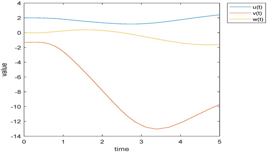
Figure 1. Simulation of solutions in Example 1.

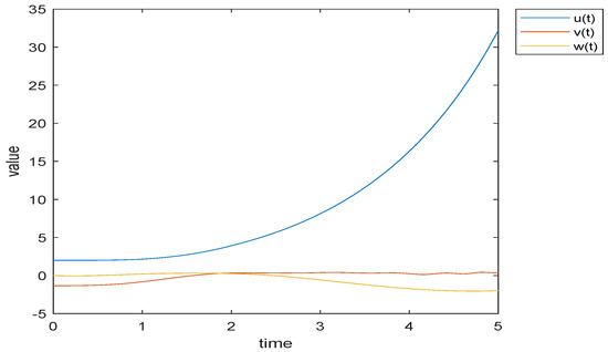
Figure 2. Simulation of solutions of the integer-order equation corresponding to Example 1.

Table 1. Comparison of numerical solutions of $u\left(t\right)$ in Example 1.

t	0	0.2	0.4	0.6	0.8	1
Fractional order	2.0000	1.9971	1.9858	1.9582	1.9033	1.8187
Integer order	2.0000	1.8101	1.6193	1.4444	1.3058	1.2184

(b) When all parameter values remain invariant, the simulations of solutions of Example 2 and its corresponding integer-order differential equation are shown as Figure 3 and Figure 4, respectively. $u\left(t\right)$ is the solution of the Langevin equation in the figures. The comparison of numerical solutions of $u\left(t\right)$ is given in Table 2. It can be seen from the simulation figures and table that the solution of the integer-order equation changes sharply, while the fractional-order equation changes gently.

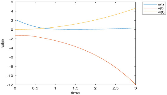
Figure 3. Simulation of solutions in Example 2.

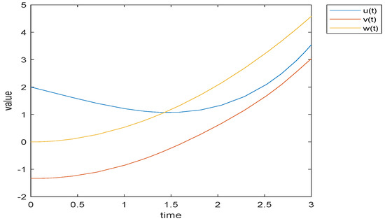
Figure 4. Simulation of solutions of the integer-order equation corresponding to Example 2.

Table 2. Comparison of numerical solutions of $u\left(t\right)$ in Example 2.

t	0	0.2	0.4	0.6	0.8	1
Fractional order	2.0000	1.4708	0.8650	0.4482	0.2147	0.1024
Integer order	2.0000	1.8100	1.6190	1.4355	1.2686	1.1276

(c) When all parameter values remain invariant, the simulations of solutions of Example 3 and its corresponding integer-order differential equation are shown as Figure 5 and Figure 6, respectively. The simulations of Ulam–Hyers stability of Example 3 is shown as Figure 7. $u\left(t\right)$ is the solution of the Langevin equation in the figures. The comparison of numerical solutions of $u\left(t\right)$ is given in Table 3 and Table 4. It can be seen from the simulation figures and tables that the solution of the integer-order equation changes sharply, while the fractional-order equation changes gently. When $ϵ\to 0^{+}$, the solution curves of Example 3 and inequality (3) almost coincide. This makes clear that Example 3 is UH-stable.

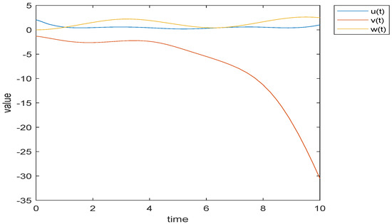
Figure 5. Simulation of solutions in Example 3.

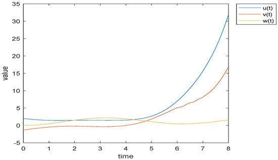
Figure 6. Simulation of solutions of the integer-order equation corresponding to Example 3.

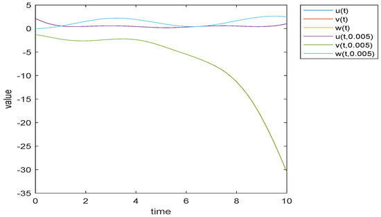
Figure 7. Simulation of UH-stability in Example 3 with $ϵ$ = 0, 0.005.

Table 3. Comparison of numerical solutions of $u\left(t\right)$ in Example 3.

t	0	0.2	0.4	0.6	0.8	1
Fractional order	2.0000	1.6614	1.2576	0.9385	0.7052	0.5470
Integer order	2.0000	1.8298	1.6924	1.5871	1.5115	1.4627

Table 4. Comparison of numerical solutions for the UH-stability of $u\left(t\right)$ in Example 3.

t	0	0.2	0.4	0.6	0.8	1
$\epsilon =0$	2.0000	1.6614	1.2576	0.9385	0.7052	0.5470
$\epsilon =0.005$	2.0000	1.6611	1.2569	0.9376	0.7042	0.5459

6. Conclusions

It is well known that the Langevin equation is a powerful tool for describing the random motion of particles in fluids. In a particularly complex viscous liquid, the integer-order Langevin equation describing the motion of particles is no longer accurate. Some scholars began to use the fractional Langevin equation as a model to study this problem and achieved good results. Most previous research on the theory and application of fractional differential systems mainly involve the Caputo- or RL-derivative. However, under certain circumstances, the Caputo- or RL-derivative is singular. To overcome this singularity, the ML-type fractional derivative is introduced. In this manuscript, we investigate the existence, uniqueness, and UH-type stability of solutions for the nonlinear ML-type fractional Langevin equation (Equation (1)). Theoretical analysis and numerical simulation of some examples verify the correctness and effectiveness of our main results. Compared with the numerical simulation of the integer-order differential equation corresponding to these examples, we find that the fractional-order differential equation is more detailed and accurate than the integer-order differential equation in describing the random motion of free particles. In practical applications, the fractional Langevin system is often affected by impulsive and random effects. Sometimes it is necessary to consider the asymptotic stability of the fractional Langevin system in the sense of Lyapunov. These are not considered in this work and need to be studied in the future.

References

- Beck, C.; Roepstorff, G. From dynamical systems to the Langevin equation. Physica A 1987, 145, 1–14. [Google Scholar] [CrossRef]
- Coffey, C.; Kalmykov, Y.; Waldron, J. The Langevin Equation; World Scientific: Singapore, 2004. [Google Scholar]
- Kubo, R. The fluctuation-dissipation theorem. Rep. Prog. Phys. 1966, 29, 255–284. [Google Scholar] [CrossRef]
- Kubo, R.; Toda, M.; Hashitsume, N. Statistical Physics II; Springer: Berlin/Heidelberg, Germany, 1991. [Google Scholar]
- Eab, C.; Lim, S. Fractional generalized langevin equation approach to single-file diffusion. Physica A 2010, 389, 2510–2521. [Google Scholar] [CrossRef]
- Sandev, T.; Tomovski, Z. Langevin equation for a free particle driven by power law type of noises. Phys. Lett. A 2014, 378, 1–9. [Google Scholar] [CrossRef]
- Jajarmi, A.; Baleanu, D.; Zarghami, V.; Pirouz, H. A new and general fractional Lagrangian approach: A capacitor microphone case study. Results Phys. 2021, 31, 104950. [Google Scholar] [CrossRef]
- Erturk, V.; Godwe, E.; Baleanu, D.; Kumar, P. Novel fractional-order Lagrangian to describe motion of beam on nanowire. Acta Phys. Pol. A 2021, 140, 265–272. [Google Scholar] [CrossRef]
- Qureshi, S.; Yusuf, A.; Aziz, S. Fractional numerical dynamics for the logistic population growth model under Conformable Caputo: A case study with real observations. Phys. Scr. 2021, 96, 114002. [Google Scholar] [CrossRef]
- Tanriverdi, T.; Baskonus, H.; Mahmud, A.; Muhamad, K.A. Explicit solution of fractional order atmosphere-soil-land plant carbon cycle system. Ecol. Complex. 2021, 48, 100966. [Google Scholar] [CrossRef]
- Abbas, M.; Ragusa, M. Solvability of Langevin equations with two Hadamard fractional derivatives via Mittag–Leffler functions. Appl. Anal. 2022, 101, 3231–3245. [Google Scholar] [CrossRef]
- Saeed, A.; Almalahi, M.; Abdo, M. Explicit iteration and unique solution for φ-Hilfer type fractional Langevin equations. AIMS Math. 2022, 7, 3456–3476. [Google Scholar] [CrossRef]
- Omaba, M.; Nwaeze, E. On a nonlinear fractional Langevin equation of two fractional orders with a multiplicative noise. Fractal Fract. 2022, 6, 290. [Google Scholar] [CrossRef]
- Almalahi, M.; Panchal, S.; Jarad, F. Multipoint BVP for the Langevin equation under φ-Hilfer fractional operator. J. Funct. Space 2022, 2022, 2798514. [Google Scholar] [CrossRef]
- Kumar, V.; Stamov, G.; Stamova, I. Controllability results for a class of piecewise nonlinear impulsive fractional dynamic systems. Appl. Math. Comput. 2022, 439, 127625. [Google Scholar] [CrossRef]
- Kou, Z.; Kosari, S. On a generalization of fractional Langevin equation with boundary conditions. AIMS Math. 2022, 7, 1333–1345. [Google Scholar] [CrossRef]
- Batiha, I.; Ouannas, A.; Albadarneh, R.; Al-Nana, A.; Momani, S. Existence and uniqueness of solutions for generalized Sturm–Liouville and Langevin equations via Caputo–Hadamard fractional-order operator. Eng. Computation 2022, 39, 2581–2603. [Google Scholar] [CrossRef]
- Ulam, S. A Collection of Mathematical Problems-Interscience Tracts in Pure and Applied Mathmatics; Interscience: New York, NY, USA, 1906. [Google Scholar]
- Hyers, D. On the stability of the linear functional equation. Proc. Nat. Acad. Sci. USA 1941, 27, 2222–2240. [Google Scholar] [CrossRef]
- Wang, J.; Li, X. A uniform method to Ulam–Hyers stability for some linear fractional equations. Mediterr. J. Math. 2016, 13, 625–635. [Google Scholar] [CrossRef]
- Rezaei, H.; Jung, S.; Rassias, T. Laplace transform and Hyers–Ulam stability of linear differential equations. J. Math. Anal. Appl. 2013, 403, 244–251. [Google Scholar] [CrossRef]
- Wang, C.; Xu, T. Hyers–Ulam stability of fractional linear differential equations involving Caputo fractional derivatives. Appl. Math. Czech. 2015, 60, 383–393. [Google Scholar] [CrossRef]
- Haq, F.; Shah, K.; Rahman, G. Hyers–Ulam stability to a class of fractional differential equations with boundary conditions. Int. J. Appl. Comput. Math. 2017, 3, 1135–1147. [Google Scholar] [CrossRef]
- Wang, J.; Zhou, Y. Nonlinear impulsive problems for fractional differential equations and Ulam stability. Comput. Math. Appl. 2012, 64, 3389–3405. [Google Scholar] [CrossRef]
- Wang, J.; Zhou, Y. Ulam’s type stability of impulsive ordinary differential equations. J. Math. Anal. Appl. 2012, 395, 258–264. [Google Scholar] [CrossRef]
- Huang, H.; Zhao, K.; Liu, X. On solvability of BVP for a coupled Hadamard fractional systems involving fractional derivative impulses. AIMS Math. 2022, 7, 19221–19236. [Google Scholar] [CrossRef]
- Wang, J.; Li, X. Eα-Ulam type stability of fractional order ordinary differential equations. J. Appl. Math. Comput. 2014, 45, 449–459. [Google Scholar] [CrossRef]
- Ibrahim, R. Generalized Ulam–Hyers stability for fractional differential equations. Int. J. Math. 2014, 23, 9. [Google Scholar] [CrossRef]
- Yu, X. Existence and β-Ulam–Hyers stability for a class of fractional differential equations with non-instantaneous impulses. Adv. Differ. Equ. 2015, 2015, 104. [Google Scholar] [CrossRef]
- Feckan, M.; Wang, J.; Zhou, Y. Presentation of solutions of impulsive fractional Langevin equations and existence results. Eur. Phys. J. Spec. Top. 2013, 222, 1857–1874. [Google Scholar]
- Wang, J.; Li, X. Ulam–Hyers stability of fractional Langevin equations. Appl. Math. Comput. 2015, 258, 72–83. [Google Scholar] [CrossRef]
- Gao, Z.; Yu, X. Stability of nonlocal fractional Langevin differential equations involving fractional integrals. J. Appl. Math. Comput. 2017, 53, 599–611. [Google Scholar] [CrossRef]
- Develi, F. Existence and Ulam–Hyers stability results for nonlinear fractional Langevin equation with modified argument. Math. Method Appl. Sci. 2022, 45, 3417–3425. [Google Scholar] [CrossRef]
- Baitiche, Z.; Derbazi, C.; Matar, M. Ulam stability for nonlinear-Langevin fractional differential equations involving two fractional orders in the psi-Caputo sense. Appl. Anal. 2021, 101, 4866–4881. [Google Scholar] [CrossRef]
- Caputo, M.; Fabrizio, M. A new definition of fractional derivative without singular kernel. Prog. Fract. Differ. Appl. 2015, 1, 73–85. [Google Scholar]
- Atangana, A.; Baleanu, D. New fractional derivatives with nonlocal and non-singular kernel: Theory and application to heat transfer model. Therm. Sci. 2016, 20, 763–769. [Google Scholar] [CrossRef]
- Sadeghi, S.; Jafari, H.; Nemati, S. Operational matrix for Atangana–Baleanu derivative based on Genocchi polynomials for solving FDEs. Chaos Soliton Fract. 2020, 135, 109736. [Google Scholar] [CrossRef]
- Ganji, R.; Jafari, H.; Baleanu, D. A new approach for solving multi variable orders differential equations with Mittag–Leffler kernel. Chaos Soliton Fract. 2020, 130, 109405. [Google Scholar] [CrossRef]
- Tajadodi, H. A numerical approach of fractional advection-diffusion equation with Atangana-Baleanu derivative. Chaos Soliton Fract. 2020, 130, 109527. [Google Scholar] [CrossRef]
- Khan, H.; Khan, A.; Jarad, F.; Shah, A. Existence and data dependence theorems for solutions of an ABC-fractional order impulsive system. Chaos Soliton Fract. 2020, 131, 109477. [Google Scholar] [CrossRef]
- Khan, H.; Li, Y.; Khan, A. Existence of solution for a fractional-order Lotka–Volterra reaction-diffusion model with Mittag–Leffler kernel. Math. Meth. Appl. Sci. 2019, 42, 3377–3387. [Google Scholar] [CrossRef]
- Acay, B.; Bas, E.; Abdeljawad, T. Fractional economic models based on market equilibrium in the frame of different type kernels. Chaos Soliton Fract. 2020, 130, 109438. [Google Scholar] [CrossRef]
- Khan, A.; Gómez-Aguilar, J.; Khan, T.; Khan, H. Stability analysis and numerical solutions of fractional order HIV/AIDS model. Chaos Soliton Fract. 2019, 122, 119–128. [Google Scholar] [CrossRef]
- Khan, H.; Gómez-Aguilar, J.; Alkhazzan, A.; Khan, A. A fractional order HIV-TB coinfection model with nonsingular Mittag–Leffler Law. Math. Meth. Appl. Sci. 2020, 43, 3786–3806. [Google Scholar] [CrossRef]
- Koca, I. Modelling the spread of Ebola virus with Atangana–Baleanu fractional operators. Eur. Phys. J. Plus 2018, 133, 100. [Google Scholar] [CrossRef]
- Morales-Delgado, V.; Gómez-Aguilar, J.; Taneco-Hernández, M.; Escobar-Jiménez, R.F.; Olivares-Peregrino, V.H. Mathematical modeling of the smoking dynamics using fractional differential equations with local and nonlocal kernel. J. Nonlinear Sci. Appl. 2018, 11, 1004–1014. [Google Scholar] [CrossRef]
- Sene, N.; Gautam, S. Generalized Mittag–Leffler input stability of the fractional differential equations. Symmetry 2019, 11, 608. [Google Scholar] [CrossRef]
- Zhao, K. Stability of a nonlinear ML-nonsingular kernel fractional Langevin system with distributed lags and integral control. Axioms 2022, 11, 350. [Google Scholar] [CrossRef]
- Zhao, K. Existence, stability and simulation of a class of nonlinear fractional Langevin equations involving nonsingular Mittag–Leffler kernel. Fractal Fract. 2022, 6, 469. [Google Scholar] [CrossRef]
- Jarad, F.; Abdeljawad, T.; Hammouch, Z. On a class of ordinary differential equations in the frame of Atangana–Baleanu fractional derivative. Chaos Soliton Fract. 2018, 117, 16–20. [Google Scholar] [CrossRef]
- Granas, A.; Dugundji, J. Fixed Point Theory; Springer: New York, NY, USA, 2003. [Google Scholar]
- Guo, D.; Lakshmikantham, V. Nonlinear Problems in Abstract Cone; Academic Press: Orlando, FL, USA, 1988. [Google Scholar]
- Shampine, L. Solving ODEs and DDEs with residual control. Appl. Numer. Math. 2005, 52, 113–127. [Google Scholar] [CrossRef]
Publisher’s Note: MDPI stays neutral with regard to jurisdictional claims in published maps and institutional affiliations. |
© 2022 by the author. Licensee MDPI, Basel, Switzerland. This article is an open access article distributed under the terms and conditions of the Creative Commons Attribution (CC BY) license (https://creativecommons.org/licenses/by/4.0/).