Computational Solution of the Time-Fractional Schrödinger Equation by Using Trigonometric B-Spline Collocation Method

Abstract

This paper proposes a numerical method to obtain an approximation solution for the time-fractional Schrödinger Equation (TFSE) based on a combination of the cubic trigonometric B-spline collocation method and the Crank-Nicolson scheme. The fractional derivative operator is described in the Caputo sense. The $L_1-$approximation method is used for time-fractional derivative discretization. Using Von Neumann stability analysis, the proposed technique is shown to be conditionally stable. Numerical examples are solved to verify the accuracy and effectiveness of this method. The error norms $L_2$ and $L_{\infty }$ are also calculated at different values of N and t to evaluate the performance of the suggested method.

1. Introduction

The nonlinear Schrödinger equation is one of the most fundamental equations of quantum physics, and can be used to describe many nonlinear phenomena such as fluid dynamics, waves in water, plasma, and self-focusing in laser pulses. Different approximation schemes have been used to investigate different kinds of nonlinear Schrödinger equations [1,2,3].

Fractional calculus is one of the most widely popular calculus types, with a vast range of applications in many different scientific and engineering disciplines. The order of derivatives in fractional calculus can be any real number, which distinguishes it from ordinary calculus, where the order of derivatives can only be natural numbers. Fractional calculus is a powerful and versatile tool for modeling a wide range of scientific phenomena, including image processing, earthquake engineering, biomedical engineering, computational fluid mechanics, and physics. In recent decades, the conventional Schrödinger equation has been generalized to a fractional order partial differential equation that takes into consideration the Riemann–Liouville, Caputo, and Riesz derivatives instead of the classical Laplacian [4,5,6,7]. The Caputo fractional derivative is considered here because it allows traditional initial and boundary conditions to be included in the formulation of the problem [8]. It is not easy to obtain the exact solutions of TFSE, although it can be found in some special cases [9,10,11,12]. In general cases, we need some convenient numerical techniques for solving the TFSE.

The approximate solutions of TFSE have been studied by many authors. Zhang et al. [13] proposed a fully discrete scheme using the $L_1$ scheme based on graded mesh for the discretiaztion of temporal Caputo derivative and the spectral method for spatial discretization for TFSE with initial singularity. Li et al. [14] solved the TFSE using a non-polynomial spline. Liu and Jiang in [15] proposed a new scheme based on the reproducing kernel theory and collocation method for solving the TFSE. Esen and Orkun [16,17] proposed a cubic B-spline collocation method and a quadratic B-spline Galerkin method to obtain the numerical solutions of TFSEs, respectively. The authors in [18] suggested the Crank–Nicolson difference algorithm for solving the time-space FSEs. Space fractional variable-order Schrödinger equation solved numerically via the Crank-Nicolson scheme by Atangana and Cloot [19]. Wei et al. [20] developed an implicit fully discrete local discontinuous Galerkin technique for solving the TFSE, and an extended method for coupled TFSEs [21]. Yaseen et al. [22] discussed the solution of the sub-diffusion equation of fractional order using a cubic trigonometric B-spline method. Bhrawya and Abdelkawy [23] developed the collocation method to solve one-and two-dimensional fractional Schrödinger equations subject to initial-boundary and non-local conditions.

The authors in [24] used a hybrid numerical method based on a cubic trigonometric B-spline to solve Fisher’s reaction-diffusion problem. Heydari and Atangana [25] used the operational matrix method based on the shifted Legendre cardinal functions for solving the nonlinear variable-order of TFSE. Erfanian, et al. in [26] applied cubic B-splines based on the finite-difference formula for solving the TFSEs. the MFVIM is used for finding approximate and exact solutions of the TFSEs by Hong [10]. Zhang et al. [27] propose a Crank-Nicolson Galerkin-Legendre spectral scheme for the one-dimensional nonlinear SFSEs. Wang and Huang [28] carried out a rigorous numerical analysis on the conservative Crank-Nicolson finite difference scheme for discretizing the SFSE with the Riesz space fractional derivative.

For the analytical solution of the nonlinear fractional Schrödinger equation, one can refer to the residual power series method [29], double Laplace transform [30], homotopy analysis transform method [31], generalized Kudryshov method [32], adomian decomposition method [33], generalized Riccati equation mapping method and the modified Kudryashov method [34], and the fractional Riccati expansion method [35].

In this paper, we applied the cubic Trigonometric B-Spline Algorithm [22,24,36] to obtain the numerical solutions of the following TFSE:

$$i\frac{{\partial }^{\alpha }u\left(x,t\right)}{\partial t^{\alpha }}+\frac{{\partial }^{2}u\left(x,t\right)}{\partial x^2}+{\left|u\left(x,t\right)\right|}^{2}u\left(x,t\right)=f\left(x,t\right),$$

(1)

subject to the initial-boundary conditions

$$u(x,0)=g\left(x\right),a\le x\le b,$$

$$u(a,t)=\Omega \left(t\right),u(b,t)=\Lambda \left(t\right),t\ge 0,$$

where $i=\sqrt{-1}$ and the fractional partial derivative of order $\alpha ,$ in Equation (1) is Caputo derivative, defined by Murio [37] and Podlubny [6],

$$\frac{{\partial }^{\alpha }u(x_i,t)}{\partial t^{\alpha }}=\frac{1}{\Gamma (n-\alpha )}\underset{t^{*}}{\overset{t}{\int }}\frac{{\partial }^{n}u(x_i,s)}{\partial t^n}{(t-s)}^{n-\alpha -1}ds.t^{*}\le t\le T,n-1<\alpha \le n,n=1,2,\cdots .$$

(2)

To obtain a finite element scheme for solving TFSE, the first-order approximation of time fractional Caputo derivative will be discretized utilizing the so-called $L1-$approximation [3,38]:

$$\frac{{\partial }^{\alpha }{U}_j^{n+1}}{\partial t^{\alpha }}={\left.\frac{{\partial }^{\alpha }U(x_j,t)}{\partial t^{\alpha }}\right|}_{t=t_{n+1}}=\frac{{\tau }^{-\alpha }}{\Gamma \left(2-\alpha \right)}\sum _{k=0}^n{\phi }_k^{\alpha }\left(U_j^{n-k+1}-U_j^{n-k}\right)+\mathcal{O}\left({\tau }^{2-\alpha }\right),$$

(3)

where $\tau =t_{n+1}-t_n$ is the time step size and ${\phi }_k^{\alpha }={\left(k+1\right)}^{1-\alpha }-k^{1-\alpha }.$

Lemma 1.

([7,14]) Let $0<\alpha <1$ and ${\phi }_k={(k+1)}^{1-\alpha }-k^{1-\alpha },k=$ $0,1,\cdots$, then $1={\phi }_0^{\alpha }>{\phi }_1^{\alpha }>\cdots >{\phi }_k^{\alpha }\to 0,$ as $k\to \infty$.

We decompose the complex functions $u(x,t)$ into its real and imaginary parts $R(x,t)$ and $S(x,t),$, respectively.

$$u(x,t)=R\left(x,t\right)+iS\left(x,t\right).$$

(4)

Substituting Equation (4) into Equation (1) results in coupled system of nonlinear partial differential equations

$$\begin{array}{cc}\hfill \frac{{\partial }^{\alpha }S}{\partial t^{\alpha }}-\frac{{\partial }^{2}R}{\partial x^2}-\left(R^2+S^2\right)R& =-f_{Re}\left(x,t\right),\hfill \end{array}$$

(5)

$$\begin{array}{cc}\hfill \frac{{\partial }^{\alpha }R}{\partial t^{\alpha }}+\frac{{\partial }^{2}S}{\partial x^2}+\left(R^2+S^2\right)S& =f_{Im}\left(x,t\right),\hfill \end{array}$$

(6)

where $f_{Re}\left(x,t\right)$ and $f_{Im}\left(x,t\right)$ are the real and imaginary parts of the $f\left(x,t\right)$, respectively. Furthermore, we have initial conditions of Equation (1) as follows:

$$R\left(x,0\right)=g_{Re}\left(x\right),S\left(x,0\right)=g_{Im}\left(x\right),a\le x\le b,$$

where $g_{Re}\left(x\right)$ and $g_{Im}\left(x\right)$ are the real and imaginary parts of $g\left(x\right)$, respectively, and the boundary conditions as

$$R(a,t)={\Omega }_{Re}\left(t\right),R(b,t)={\Lambda }_{Re}\left(t\right),S(a,t)={\Omega }_{Im}\left(t\right),S(b,t)={\Lambda }_{Im}\left(t\right),t\ge 0,$$

where ${\Omega }_{Re}\left(t\right)$ and ${\Omega }_{Im}\left(t\right)$ are the real and imaginary parts of the $\Omega \left(t\right)$, respectively, and ${\Lambda }_{Re}\left(t\right)$ and ${\Lambda }_{Im}\left(t\right)$ are the real and imaginary parts of the $\Lambda \left(t\right)$, respectively.

2. Derivation of the Numerical Method

Consider Equation (1) and assume that $a=x_0<x_1<x_2<\cdots <x_N=b,$ be N uniform divides of the interval $[a,b]$ with space step size $h=\frac{b-a}{N}$ and $t_{j+1}-t_j=\tau ,t_n=n\tau$, where $n=0,1,\dots .$ The cubic trigonometric B-spline basis functions $CT{B}_j\left(x\right)$ at the knots $x_j$ are given by:

$$CT{B}_j\left(x\right)=\frac{1}{\theta }\left\{\begin{array}{cc}{\omega }_{j-2}^3\left(x\right),& x_{j-2}\le x\le x_{j-1},\hfill \\ {\omega }_{j-2}\left(x\right)({\omega }_{j-2}\left(x\right){\varphi }_j\left(x\right)+{\omega }_{j-1}\left(x\right){\varphi }_{j+1}\left(x\right))+{\omega }_{j-1}^2\left(x\right){\varphi }_{j+1}\left(x\right),& x_{j-1}\le x\le x_j,\hfill \\ {\omega }_{j-2}\left(x\right){\varphi }_{j+1}^2\left(x\right)+{\varphi }_{j+2}\left(x\right)({\omega }_{j-1}\left(x\right){\varphi }_{j+1}\left(x\right)+{\omega }_j\left(x\right){\varphi }_{j+2}\left(x\right)),& x_j\le x\le x_{j+1},\hfill \\ {\varphi }_{j+2}^3\left(x\right),& x_{j+1}\le x\le x_{j+2},\hfill \\ 0,& Othrewise,\hfill \end{array}\right.$$

where ${\omega }_j=sin\left(\frac{x-x_j}{2}\right),{\varphi }_j=sin\left(\frac{x_j-x}{2}\right),\mathrm{and}\theta =sin\left(\frac{h}{2}\right)sin\left(h\right)sin\left(\frac{3h}{2}\right)$.

The values of $CTB$ and their first and second derivatives at notes points are given by Table 1.

Table 1. $CTB$ and their first and second derivatives.

x	${\mathit{x}}_{\mathit{j}-2}$	${\mathit{x}}_{\mathit{j}-1}$	${\mathit{x}}_{\mathit{j}}$	${\mathit{x}}_{\mathit{j}+1}$	${\mathit{x}}_{\mathit{j}+2}$
$CT{B}_j$	0	${\alpha }_1$	${\alpha }_2$	${\alpha }_1$	0
$CT{B}_j^{\prime }$	0	${\beta }_1$	0	${\beta }_2$	0
$CT{B}_j^{″}$	0	${\gamma }_1$	${\gamma }_2$	${\gamma }_1$	0

where ${\alpha }_1={sin}^2\left(\frac{h}{2}\right)csc\left(h\right)csc\left(\frac{3h}{2}\right),{\alpha }_2=\frac{2}{1+2cos\left(h\right)},{\beta }_1=-\frac{3}{4}csc\left(\frac{3h}{2}\right),{\beta }_2=\frac{3}{4}csc\left(\frac{3h}{2}\right),$${\gamma }_1=\frac{3(1+3cos\left(h\right)){csc}^2\left(\frac{h}{2}\right)}{16(2cos\left(\frac{h}{2}\right)+cos\left(\frac{3h}{2}\right))}$, and ${\gamma }_2=\frac{-3{cot}^2\left(\frac{h}{2}\right)}{2+4cos\left(h\right)}.$

Let $R\left(x,t\right)=R_j^n$ and $S\left(x,t\right)=S_j^n$ be an approximations solutions of R and S, respectively, then from Equation (3)

$$\begin{array}{cc}\hfill \frac{{\partial }^{\alpha }{S}_j^{n+1}}{\partial t^{\alpha }}& =\frac{1}{{\tau }^{\alpha }\Gamma \left(2-\alpha \right)}\sum _{k=0}^n{\phi }_k^{\alpha }\left(S_j^{n-k+1}-S_j^{n-k}\right),\hfill \end{array}$$

(7)

$$\begin{array}{cc}\hfill \frac{{\partial }^{\alpha }{R}_j^{n+1}}{\partial t^{\alpha }}& =\frac{1}{{\tau }^{\alpha }\Gamma \left(2-\alpha \right)}\sum _{k=0}^n{\phi }_k^{\alpha }\left(R_j^{n-k+1}-R_j^{n-k}\right),\hfill \end{array}$$

(8)

Substituting Equations (7) and (8) and by implementing Crank-Nicolson scheme to Equations (5) and (6) we obtain

$$\begin{array}{cc}{S}_j^{n+1}-S_j^n+\sum _{k=1}^n{\phi }_k^{\alpha }\left(S_j^{n-k+1}-S_j^{n-k}\right)\hfill & -\eta \left({\left(R_{xx}\right)}_j^{n+1}+{\left(R_{xx}\right)}_j^n\right)\hfill \\ & -\eta \left({\left(R^3\right)}_j^{n+1}+{\left(R^3\right)}_j^n+{\left(S^{2}R\right)}_j^{n+1}+{\left(S^{2}R\right)}_j^n\right)=-2\eta {\left(f_{Re}\right)}_j^n,\hfill \end{array}$$

(9)

$$\begin{array}{cc}{R}_j^{n+1}-R_j^n+\sum _{k=1}^n{\phi }_k^{\alpha }\left(R_j^{n-k+1}-R_j^{n-k}\right)\hfill & +\eta \left({\left(S_{xx}\right)}_j^{n+1}+{\left(S_{xx}\right)}_j^n\right)\hfill \\ & +\eta \left({\left(R^{2}S\right)}_j^{n+1}+{\left(R^{2}S\right)}_j^n+{\left(S^3\right)}_j^{n+1}+{\left(S^3\right)}_j^n\right)=2\eta {\left(f_{Im}\right)}_j^n,\end{array}$$

(10)

where $\eta =\frac{{\tau }^{\alpha }\Gamma \left(2-\alpha \right)}{2},$ the nonlinear terms in Equations (9) and (10) are linearized using the form given by Rubin and Graves [39] as: ${\left(SR\right)}_j^{n+1}=S_j^{n+1}{R}_j^n+S_j^n{R}_j^{n+1}-S_j^n{R}_j^n,$ thus we obtain the following equations

$$\begin{array}{cc}\hfill S_j^{n+1}-\eta {\left(R_{xx}\right)}_j^{n+1}& -3\eta {\left(R_j^n\right)}^2{R}_j^{n+1}-2\eta S_j^n{R}_j^n{S}_j^{n+1}-\eta {\left(S_j^n\right)}^2{R}_j^{n+1}=\hfill \\ & -\eta {\left(R_j^n\right)}^3-\eta {\left(S_j^n\right)}^2{R}_j^n+\eta {\left(R_{xx}\right)}_j^n+S_j^n-\sum _{k=1}^n{\phi }_k^{\alpha }\left(S_j^{n-k+1}-S_j^{n-k}\right)-2\eta {\left(f_{Re}\right)}_j^n,\hfill \end{array}$$

(11)

$$\begin{array}{cc}{R}_j^{n+1}+\eta {\left(S_{xx}\right)}_j^{n+1}\hfill & +3\eta {\left(S_j^n\right)}^2{S}_j^{n+1}+2\eta S_j^n{R}_j^n{R}_j^{n+1}+\eta {\left(R_j^n\right)}^2{S}_j^{n+1}=\hfill \\ & \eta {\left(S_j^n\right)}^3+\eta {\left(R_j^n\right)}^2{S}_j^n-\eta {\left(S_{xx}\right)}_j^n+R_j^n-\sum _{k=1}^n{\phi }_k^{\alpha }\left(R_j^{n-k+1}-R_j^{n-k}\right)+2\eta {\left(f_{Im}\right)}_j^n.\hfill \end{array}$$

(12)

After some simple arrangements for Equations (11) and (12), we obtain

$$\begin{array}{cc}\hfill Z_1{S}_j^{n+1}-\eta {\left(R_{xx}\right)}_j^{n+1}+Z_2{R}_j^{n+1}& =-\eta \left({\left(R_j^n\right)}^2+{\left(S_j^n\right)}^2\right)R_j^n\hfill \\ & +\eta {\left(R_{xx}\right)}_j^n+S_j^n-\sum _{k=1}^n{\phi }_k^{\alpha }\left(S_j^{n-k+1}-S_j^{n-k}\right)-2\eta {\left(f_{Re}\right)}_j^n,\hfill \end{array}$$

(13)

$$\begin{array}{cc}\hfill Z_3{R}_j^{n+1}+\eta {\left(S_{xx}\right)}_j^{n+1}+Z_4{S}_j^{n+1}& =\eta \left({\left(S_j^n\right)}^2+{\left(R_j^n\right)}^2\right)S_j^n\hfill \\ & -\eta {\left(S_{xx}\right)}_j^n+R_j^n-\sum _{k=1}^n{\phi }_k^{\alpha }\left(R_j^{n-k+1}-R_j^{n-k}\right)+2\eta {\left(f_{Im}\right)}_j^n,\hfill \end{array}$$

(14)

where $Z_1=1-2\eta S_j^n{R}_j^n,Z_2=-\eta \left({\left(S_j^n\right)}^2+3{\left(R_j^n\right)}^2\right),Z_3=1+2\eta S_j^n{R}_j^n,$ and $Z_4=\eta \left(3{\left(S_j^n\right)}^2+{\left(R_j^n\right)}^2\right).$

The approximate solution of $S(x,t)$ and $R(x,t)$ can be written in terms of $CT{B}_j\left(x\right)$ and the unknown weighting coefficients ${\sigma }_j\left(t\right)$ and ${\delta }_j\left(t\right)$, respectively, as follows:

$$R_N(x,t)=\stackrel{N+1}{\sum _{j=-1}}{\delta }_j\left(t\right)CT{B}_j\left(x\right),S_N(x,t)=\stackrel{N+1}{\sum _{j=-1}}{\sigma }_j\left(t\right)CT{B}_j\left(x\right).$$

(15)

Using Equation (15) and values of $CT{B}_j$ shown in Table 1, the approximate solutions of $R,S$ and their derivatives are determined according to the time parameters as follows:

$$\begin{array}{c}\hfill \left.\begin{array}{c}{S}_j=S\left(x_j\right)={\alpha }_1{\sigma }_{j-1}+{\alpha }_2{\sigma }_j+{\alpha }_1{\sigma }_{j+1},\hfill \\ S_j^{\prime }=S^{\prime }\left(x_j\right)={\beta }_1{\sigma }_{j-1}+{\beta }_2{\sigma }_{j+1},\hfill \\ S_j^{″}=S^{″}\left(x_j\right)={\gamma }_1{\sigma }_{j-1}+{\gamma }_2{\sigma }_j+{\gamma }_1{\sigma }_{j+1},\hfill \end{array}\right\},\end{array}$$

(16)

$$\begin{array}{c}\hfill \left.\begin{array}{c}{R}_j=R\left(x_j\right)={\alpha }_1{\delta }_{j-1}+{\alpha }_2{\delta }_j+{\alpha }_1{\delta }_{j+1},\hfill \\ R_j^{\prime }=R^{\prime }\left(x_j\right)={\beta }_1{\delta }_{j-1}+{\beta }_2{\delta }_{j+1},\hfill \\ R_j^{″}=R^{″}\left(x_j\right)={\gamma }_1{\delta }_{j-1}+{\gamma }_2{\delta }_j+{\gamma }_1{\delta }_{j+1},\hfill \end{array}\right\}.\end{array}$$

(17)

Substituting Equations (16) and (17) into Equations (13) and (14), we obtain a recurrence scheme with unknown parameters ${\delta }_j^n$ and ${\sigma }_j^n$ as follows:

$$\begin{array}{cccc}\hfill {\alpha }_1{Z}_1{\sigma }_{j-1}^1+{\alpha }_2{Z}_1{\sigma }_j^1+{\alpha }_1{Z}_1{\sigma }_{j+1}^1+A_1{\delta }_{j-1}^1& +A_2{\delta }_j^1+A_1{\delta }_{j+1}^1=B_1{\delta }_{j-1}^0+B_2{\delta }_j^0\hfill & & \\ & +B_1{\delta }_{j+1}^0+{\alpha }_1{\sigma }_{j-1}^0+{\alpha }_2{\sigma }_j^0+{\alpha }_1{\sigma }_{j+1}^0-2\eta {\left(f_{Re}\right)}_j^0,\hfill & & \end{array}$$

(18)

$$\begin{array}{cccc}\hfill {\alpha }_1{Z}_3{\delta }_{j-1}^1+{\alpha }_2{Z}_3{\delta }_j^1+{\alpha }_1{Z}_3{\delta }_{j+1}^1+A_3{\sigma }_{j-1}^1& +A_4{\sigma }_j^1+A_3{\sigma }_{j+1}^1=-B_1{\sigma }_{j-1}^0-B_2{\sigma }_j^0\hfill & & \hfill \\ & -B_1{\sigma }_{j+1}^0+{\alpha }_1{\delta }_{j-1}^0+{\alpha }_2{\delta }_j^0+{\alpha }_1{\delta }_{j+1}^0+2\eta {\left(f_{Im}\right)}_j^0,\hfill \end{array}$$

(19)

$$\begin{array}{cccc}\hfill {\alpha }_1{Z}_1{\sigma }_{j-1}^{n+1}+{\alpha }_2{Z}_1{\sigma }_j^{n+1}& +{\alpha }_1{Z}_1{\sigma }_{j+1}^{n+1}+A_1{\delta }_{j-1}^{n+1}+A_2{\delta }_j^{n+1}+A_1{\delta }_{j+1}^{n+1}\hfill & & \\ & =B_1{\delta }_{j-1}^n+B_2{\delta }_j^n+B_1{\delta }_{j+1}^n+{\alpha }_1{\sigma }_{j-1}^n+{\alpha }_2{\sigma }_j^n+{\alpha }_1{\sigma }_{j+1}^n-2\eta {\left(f_{Re}\right)}_j^n\hfill & & \\ & -\sum _{k=1}^n{\phi }_k^{\alpha }\left({\alpha }_1\left({\sigma }_{j-1}^{n-k+1}-{\sigma }_{j-1}^{n-k}\right)+{\alpha }_2\left({\sigma }_j^{n-k+1}-{\sigma }_j^{n-k}\right)+{\alpha }_1\left({\sigma }_{j+1}^{n-k+1}-{\sigma }_{j+1}^{n-k}\right)\right),\hfill & & \end{array}$$

(20)

$$\begin{array}{cccc}\hfill {\alpha }_1{Z}_3{\delta }_{j-1}^{n+1}+{\alpha }_2{Z}_3{\delta }_j^{n+1}& +{\alpha }_1{Z}_3{\delta }_{j+1}^{n+1}+A_3{\sigma }_{j-1}^{n+1}+A_4{\sigma }_j^{n+1}+A_3{\sigma }_{j+1}^{n+1}\hfill & & \hfill \\ & =-B_1{\sigma }_{j-1}^n-B_2{\sigma }_j^n-B_1{\sigma }_{j+1}^n+{\alpha }_1{\delta }_{j-1}^n+{\alpha }_2{\delta }_j^n+{\alpha }_1{\delta }_{j+1}^n+2\eta {\left(f_{Im}\right)}_j^n\hfill & & \\ & -\sum _{k=1}^n{\phi }_k^{\alpha }\left({\alpha }_1\left({\delta }_{j-1}^{n-k+1}-{\delta }_{j-1}^{n-k}\right)+{\alpha }_2\left({\delta }_j^{n-k+1}-{\delta }_j^{n-k}\right)+{\alpha }_1\left({\delta }_{j+1}^{n-k+1}-{\delta }_{j+1}^{n-k}\right)\right),\hfill \end{array}$$

(21)

where $A_1={\alpha }_1{Z}_2-\eta {\gamma }_1,A_2={\alpha }_2{Z}_2-\eta {\gamma }_2,A_3={\alpha }_1{Z}_4+\eta {\gamma }_1,$$A_4={\alpha }_2{Z}_4+\eta {\gamma }_2,$$B_1=\eta \left({\gamma }_1-{\alpha }_1\left({\left(S_j^n\right)}^2+{\left(R_j^n\right)}^2\right)\right)$ and $B_2=\eta \left({\gamma }_2-{\alpha }_2\left({\left(S_j^n\right)}^2+{\left(R_j^n\right)}^2\right)\right),j=0,1,\cdots ,N,$$n\ge 1.$

Equations (18)–(21) yields a system consisting of $2N+2$ equations with $2N+6$ unknowns $({\sigma }_{-1},{\sigma }_0,\cdots ,{\sigma }_{N+1}$, ${\delta }_{-1},{\delta }_0,\cdots ,{\delta }_{N+1}{)}^T,$ four additional constraints are required to obtain a unique solution to the resulting system. These are obtained by imposing boundary conditions.

$$S_0=S(x_0,t)={\Omega }_{Im}\left(t\right)={\alpha }_1{\sigma }_{-1}\left(t\right)+{\alpha }_2{\sigma }_0\left(t\right)+{\alpha }_1{\sigma }_1\left(t\right),$$

$$R_0=R(x_0,t)={\Omega }_{Re}\left(t\right)={\alpha }_1{\delta }_{-1}\left(t\right)+{\alpha }_2{\delta }_0\left(t\right)+{\alpha }_1{\delta }_1\left(t\right),$$

$$S_N=S(x_N,t)={\Lambda }_{Im}\left(t\right)={\alpha }_1{\sigma }_{N-1}\left(t\right)+{\alpha }_2{\sigma }_N\left(t\right)+{\alpha }_1{\sigma }_{N+1}\left(t\right),$$

$$R_N=R(x_N,t)={\Lambda }_{Re}\left(t\right)={\alpha }_1{\delta }_{N-1}\left(t\right)+{\alpha }_2{\delta }_N\left(t\right)+{\alpha }_1{\delta }_{N+1}\left(t\right).$$

These conditions are used to eliminate ${\sigma }_{-1},{\sigma }_{N+1},{\delta }_{-1},{\delta }_{N+1}$ from Equations (18)–(21) . The initial conditions and their first derivatives are used to obtain initial vectors ${\sigma }_j^0$ and ${\delta }_j^0$, as follows

$$S_j^0=S(x_j,0)=g_{Im}\left(x_j\right)={\alpha }_1{\sigma }_{j-1}^0+{\alpha }_2{\sigma }_j^0+{\alpha }_1{\sigma }_{j+1}^0,$$

$${\left(S_0^0\right)}^{\prime }=S^{\prime }(x_0,0)=g_{Im}^{\prime }\left(x_0\right)={\beta }_1{\sigma }_{-1}^0+{\beta }_2{\sigma }_1^0,$$

$${\left(S_N^0\right)}^{\prime }=S^{\prime }(x_N,0)=g_{Im}^{\prime }\left(x_N\right)={\beta }_1{\sigma }_{N-1}^0+{\beta }_2{\sigma }_{N+1}^0,$$

$$R_j^0=R(x_j,0)=g_{Re}\left(x_j\right)={\alpha }_1{\delta }_{j-1}^0+{\alpha }_2{\delta }_j^0+{\alpha }_1{\delta }_{j+1}^0,$$

$${\left(R_0^0\right)}^{\prime }=R^{\prime }(x_0,0)=g_{Re}^{\prime }\left(x_0\right)={\beta }_1{\delta }_{-1}^0+{\beta }_2{\delta }_1^0,$$

$${\left(R_N^0\right)}^{\prime }=R^{\prime }(x_N,0)=g_{Re}^{\prime }\left(x_N\right)={\beta }_1{\delta }_{N-1}^0+{\beta }_2{\delta }_{N+1}^0,$$

which can be resolved using a proper algorithm.

3. Stability Analysis

In this section, we use the Von Neumann method to analyze the stability of the scheme (18)–(21). First, we linearize the nonlinear terms R and S as local constants ${\lambda }_1$ and ${\lambda }_2$, respectively, as is done in the Von Neumann method. According to Duhamel’s principle, the stability analysis for an inhomogeneous problem is assumed to be an immediate outcome of the stability analysis for the corresponding homogeneous case. Therefore, the stability analysis for the scheme (18)–(21) for the force-free situation ($f_{Re}=f_{Im}=0$) is sufficient.

Let ${E_{\sigma }}_j^{n+1}={\sigma }_j^{n+1}-{\tilde{\sigma }}_j^{n+1}$ and ${E_{\delta }}_j^{n+1}={\delta }_j^{n+1}-{\tilde{\delta }}_j^{n+1}$ where ${\tilde{\sigma }}_j^{n+1}$ and ${\tilde{\delta }}_j^{n+1}$ are the approximate solutions of system (18)–(21), we can easily obtain the following round-off error equations

$$\begin{array}{cccc}\hfill {\alpha }_1{Z}_1{E_{\sigma }}_{j-1}^1+{\alpha }_2{Z}_1{E_{\sigma }}_j^1& +{\alpha }_1{Z}_1{E_{\sigma }}_{j+1}^1+A_1{E_{\delta }}_{j-1}^1+A_2{E_{\delta }}_j^1+A_1{E_{\delta }}_{j+1}^1=B_1{E_{\delta }}_{j-1}^0\hfill & & \\ & +B_2{E_{\delta }}_j^0+B_1{E_{\delta }}_{j+1}^0+{\alpha }_1{E_{\sigma }}_{j-1}^0+{\alpha }_2{E_{\sigma }}_j^0+{\alpha }_1{E_{\sigma }}_{j+1}^0,\hfill & & \end{array}$$

(22)

$$\begin{array}{cc}{\alpha }_1{Z}_3{E_{\delta }}_{j-1}^1+{\alpha }_2{Z}_3{E_{\delta }}_j^1\hfill & +{\alpha }_1{Z}_3{E_{\delta }}_{j+1}^1+A_3{E_{\sigma }}_{j-1}^1+A_4{E_{\sigma }}_j^1+A_3{E_{\sigma }}_{j+1}^1=-B_1{E_{\sigma }}_{j-1}^0\hfill \\ & -B_2{E_{\sigma }}_j^0-B_1{E_{\sigma }}_{j+1}^0+{\alpha }_1{E_{\delta }}_{j-1}^0+{\alpha }_2{E_{\delta }}_j^0+{\alpha }_1{E_{\delta }}_{j+1}^0,\hfill \end{array}$$

(23)

$$\begin{array}{cccc}\hfill {\alpha }_1{Z}_1{E_{\sigma }}_{j-1}^{n+1}+{\alpha }_2{Z}_1{E_{\sigma }}_j^{n+1}& +{\alpha }_1{Z}_1{E_{\sigma }}_{j+1}^{n+1}+A_1{E_{\delta }}_{j-1}^{n+1}+A_2{E_{\delta }}_j^{n+1}\hfill & & \\ & +A_1{E_{\delta }}_{j+1}^{n+1}=B_1{E_{\delta }}_{j-1}^n+B_2{E_{\delta }}_j^n+B_1{E_{\delta }}_{j+1}^n+{\alpha }_1{E_{\sigma }}_{j-1}^n+{\alpha }_2{E_{\sigma }}_j^n+{\alpha }_1{E_{\sigma }}_{j+1}^n\hfill & & \\ & -\sum _{k=1}^n{\phi }_k^{\alpha }\left({\alpha }_1\left({E_{\sigma }}_{j-1}^{n-k+1}-{E_{\sigma }}_{j-1}^{n-k}\right)+{\alpha }_2\left({E_{\sigma }}_j^{n-k+1}-{E_{\sigma }}_j^{n-k}\right)+{\alpha }_1\left({E_{\sigma }}_{j+1}^{n-k+1}-{E_{\sigma }}_{j+1}^{n-k}\right)\right),\hfill \end{array}$$

(24)

$$\begin{array}{cccc}\hfill {\alpha }_1{Z}_3{E_{\delta }}_{j-1}^{n+1}+{\alpha }_2{Z}_3{E_{\delta }}_j^{n+1}& +{\alpha }_1{Z}_3{E_{\delta }}_{j+1}^{n+1}+A_3{E_{\sigma }}_{j-1}^{n+1}+A_4{E_{\sigma }}_j^{n+1}\hfill & & \hfill \\ & +A_3{E_{\sigma }}_{j+1}^{n+1}=-B_1{E_{\sigma }}_{j-1}^n-B_2{E_{\sigma }}_j^n-B_1{E_{\sigma }}_{j+1}^n+{\alpha }_1{E_{\delta }}_{j-1}^n+{\alpha }_2{E_{\delta }}_j^n+{\alpha }_1{E_{\delta }}_{j+1}^n\hfill & & \\ & -\sum _{k=1}^n{\phi }_k^{\alpha }\left({\alpha }_1\left({E_{\delta }}_{j-1}^{n-k+1}-{E_{\delta }}_{j-1}^{n-k}\right)+{\alpha }_2\left({E_{\delta }}_j^{n-k+1}-{E_{\delta }}_j^{n-k}\right)+{\alpha }_1\left({E_{\delta }}_{j+1}^{n-k+1}-{E_{\delta }}_{j+1}^{n-k}\right)\right),\hfill \end{array}$$

(25)

where $Z_1=1-2\eta {\lambda }_1{\lambda }_2,Z_2=-\eta \left({\lambda }_2^2+3{\lambda }_1^2\right),Z_3=1+2\eta {\lambda }_1{\lambda }_2$ and $Z_4=\eta \left(3{\lambda }_2^2+{\lambda }_1^2\right).$

Suppose that Equations (22)–(25) have solutions of the form

$$\begin{array}{c}\hfill {E_{\sigma }}_j^n={\xi }_n{e}^{ij\varphi h},{E_{\delta }}_j^n={\zeta }_n{e}^{ij\varphi h},n\ge 0,\end{array}$$

(26)

where $i=\sqrt{-1}$ and $\varphi$ is real. Substituting Equation (26) into Equations (22)–(25), dividing by $e^{ij\varphi h}$, using the relation and collecting the like terms, we obtain

$$\begin{array}{cccc}\hfill & {\xi }_1{Z}_1\left(2{\alpha }_{1}cos\left(\varphi h\right)+{\alpha }_2\right)+{\zeta }_1\left(2A_{1}cos\left(\varphi h\right)+A_2\right)={\zeta }_0\left(2B_{1}cos\left(\varphi h\right)+B_2\right)+{\xi }_0\left(2{\alpha }_{1}cos\left(\varphi h\right)+{\alpha }_2\right),\hfill & & \end{array}$$

(27)

$$\begin{array}{ccc}{\zeta }_1{Z}_3\left(2{\alpha }_{1}cos\left(\varphi h\right)+{\alpha }_2\right)+{\xi }_1\left(2A_{3}cos\left(\varphi h\right)+A_4\right)=-{\xi }_0\left(2B_{1}cos\left(\varphi h\right)+B_2\right)+{\zeta }_0\left(2{\alpha }_{1}cos\left(\varphi h\right)+{\alpha }_2\right),\hfill & & \\ {\xi }_{n+1}{Z}_1\left(2{\alpha }_{1}cos\left(\varphi h\right)+{\alpha }_2\right)+{\zeta }_{n+1}\left(2A_{1}cos\left(\varphi h\right)+A_2\right)={\zeta }_n\left(2B_{1}cos\left(\varphi h\right)+B_2\right)\hfill & & \end{array}$$

(28)

$$\begin{array}{cccc}& +\left(2{\alpha }_{1}cos\left(\varphi h\right)+{\alpha }_2\right)\left({\xi }_n-\sum _{k=1}^n{\phi }_k^{\alpha }\left({\xi }_{n-k+1}-{\xi }_{n-k}\right)\right),\hfill & & \end{array}$$

(29)

$$\begin{array}{cccc}\hfill & {\zeta }_{n+1}{Z}_3\left(2{\alpha }_{1}cos\left(\varphi h\right)+{\alpha }_2\right)+{\xi }_{n+1}\left(2A_{3}cos\left(\varphi h\right)+A_4\right)=-{\xi }_n\left(2B_{1}cos\left(\varphi h\right)+B_2\right)\hfill & & \\ & +\left(2{\alpha }_{1}cos\left(\varphi h\right)+{\alpha }_2\right)\left({\zeta }_n-\sum _{k=1}^n{\phi }_k^{\alpha }\left({\zeta }_{n-k+1}-{\zeta }_{n-k}\right)\right).\hfill \end{array}$$

(30)

Substituting values of $A_1,A_2,A_3,A_4,B_1$ and $B_2$ in Equations (27)–(30), and after some rearrangement and dividing by $\left(2{\alpha }_{1}cos\left(\varphi h\right)+{\alpha }_2\right)$, we obtain

$$\begin{array}{cc}\hfill & Z_1{\xi }_1+\left(Z_2-\eta {\rm Y}\right){\zeta }_1={\xi }_0-\left(Z_5-\eta {\rm Y}\right){\zeta }_0,\hfill \end{array}$$

(31)

$$\begin{array}{cc}\hfill & \left(\eta {\rm Y}+Z_4\right){\xi }_1+Z_3{\zeta }_1={\zeta }_0+\left(Z_5-\eta {\rm Y}\right){\xi }_0,\hfill \end{array}$$

(32)

$$\begin{array}{cc}\hfill & Z_1{\xi }_{n+1}+\left(Z_2-\eta {\rm Y}\right){\zeta }_{n+1}=-\left(Z_5-\eta {\rm Y}\right){\zeta }_n+\left({\xi }_n-\sum _{k=1}^n{\phi }_k^{\alpha }\left({\xi }_{n-k+1}-{\xi }_{n-k}\right)\right),\hfill \end{array}$$

(33)

$$\begin{array}{cc}\hfill & \left(\eta {\rm Y}+Z_4\right){\xi }_{n+1}+Z_3{\zeta }_{n+1}=\left(Z_5-\eta {\rm Y}\right){\xi }_n+\left({\zeta }_n-\sum _{k=1}^n{\phi }_k^{\alpha }\left({\zeta }_{n-k+1}-{\zeta }_{n-k}\right)\right),\hfill \end{array}$$

(34)

where $n=1,2,3,\cdots ,{\rm Y}=\frac{2{\gamma }_{1}cos\left(\varphi h\right)+{\gamma }_2}{2{\alpha }_{1}cos\left(\varphi h\right)+{\alpha }_2}$ and $Z_5=\eta \left({\lambda }_1^2+{\lambda }_2^2\right).$

Using Wolfram Mathematica to solve the last system, we obtain

$$\begin{array}{cccc}& {\xi }_1=\frac{2{\zeta }_0\eta \left({\lambda }_2\left({\lambda }_2-\eta {\lambda }_1\left(-{\rm Y}+{\lambda }_1^2+{\lambda }_2^2\right)\right)+{\rm Y}\right)}{{{\rm Y}}^2{\eta }^2+{\eta }^2\left({\lambda }_1^2+{\lambda }_2^2\right)\left(4{\rm Y}+3{\lambda }_1^2+3{\lambda }_2^2\right)+1}+\frac{{\xi }_0\left(\eta \left(\eta \left({\lambda }_1^4-{{\rm Y}}^2\right)-2\eta {\lambda }_2^2\left({\rm Y}-2{\lambda }_1^2\right)+3\eta {\lambda }_2^4+2{\lambda }_1{\lambda }_2\right)+1\right)}{{{\rm Y}}^2{\eta }^2+{\eta }^2\left({\lambda }_1^2+{\lambda }_2^2\right)\left(4{\rm Y}+3{\lambda }_1^2+3{\lambda }_2^2\right)+1},\hfill & & \\ & {\zeta }_1=\frac{{\zeta }_0\left(-{{\rm Y}}^2{\eta }^2+\eta \left(-2\eta {\lambda }_1^2\left({\rm Y}-2{\lambda }_2^2\right)+3\eta {\lambda }_1^4+\eta {\lambda }_2^4-2{\lambda }_2{\lambda }_1\right)+1\right)}{{{\rm Y}}^2{\eta }^2+{\eta }^2\left({\lambda }_1^2+{\lambda }_2^2\right)\left(4{\rm Y}+3{\lambda }_1^2+3{\lambda }_2^2\right)+1}+\frac{2\eta {\xi }_0\left(-{\lambda }_1\left(\eta {\lambda }_2\left({\lambda }_1^2-{\rm Y}\right)+\eta {\lambda }_2^3+{\lambda }_1\right)-{\rm Y}\right)}{{{\rm Y}}^2{\eta }^2+{\eta }^2\left({\lambda }_1^2+{\lambda }_2^2\right)\left(4{\rm Y}+3{\lambda }_1^2+3{\lambda }_2^2\right)+1},\hfill & & \\ & {\xi }_{n+1}=-\frac{{\zeta }_n\left(\eta \left(-{\rm Y}+{\lambda }_1^2+{\lambda }_2^2\right)\left(2\eta {\lambda }_1{\lambda }_2+1\right)-\eta \left({\rm Y}+{\lambda }_1^2+3{\lambda }_2^2\right)\right)}{{{\rm Y}}^2{\eta }^2+{\eta }^2\left({\lambda }_1^2+{\lambda }_2^2\right)\left(4{\rm Y}+3{\lambda }_1^2+3{\lambda }_2^2\right)+1}-\frac{{\xi }_n\left({\eta }^2\left({\rm Y}-{\lambda }_1^2-{\lambda }_2^2\right)\left({\rm Y}+{\lambda }_1^2+3{\lambda }_2^2\right)-2\eta {\lambda }_1{\lambda }_2-1\right)}{{{\rm Y}}^2{\eta }^2+{\eta }^2\left({\lambda }_1^2+{\lambda }_2^2\right)\left(4{\rm Y}+3{\lambda }_1^2+3{\lambda }_2^2\right)+1}\hfill & & \\ & -\frac{\eta \left({\rm Y}+{\lambda }_1^2+3{\lambda }_2^2\right){\sum }_{k=1}^n{\psi }_k^{\alpha }\left({\zeta }_{-k+n+1}-{\zeta }_{n-k}\right)+\left(2\eta {\lambda }_1{\lambda }_2+1\right){\sum }_{k=1}^n{\psi }_k^{\alpha }\left({\xi }_{-k+n+1}-{\xi }_{n-k}\right)}{{{\rm Y}}^2{\eta }^2+{\eta }^2\left({\lambda }_1^2+{\lambda }_2^2\right)\left(4{\rm Y}+3{\lambda }_1^2+3{\lambda }_2^2\right)+1},\hfill & & \\ & {\zeta }_{n+1}=\frac{{\zeta }_n\left(-{{\rm Y}}^2{\eta }^2+\eta \left(-2\eta {\lambda }_1^2\left({\rm Y}-2{\lambda }_2^2\right)+3\eta {\lambda }_1^4+\eta {\lambda }_2^4-2{\lambda }_2{\lambda }_1\right)+1\right)}{{{\rm Y}}^2{\eta }^2+{\eta }^2\left({\lambda }_1^2+{\lambda }_2^2\right)\left(4{\rm Y}+3{\lambda }_1^2+3{\lambda }_2^2\right)+1}+\frac{2\eta {\xi }_n\left(-{\lambda }_1\left(\eta {\lambda }_2\left({\lambda }_1^2-{\rm Y}\right)+\eta {\lambda }_2^3+{\lambda }_1\right)-{\rm Y}\right)}{{{\rm Y}}^2{\eta }^2+{\eta }^2\left({\lambda }_1^2+{\lambda }_2^2\right)\left(4{\rm Y}+3{\lambda }_1^2+3{\lambda }_2^2\right)+1}\hfill & & \\ & +\frac{\eta \left({\rm Y}+3{\lambda }_1^2+{\lambda }_2^2\right){\sum }_{k=1}^n{\psi }_k^{\alpha }\left({\xi }_{-k+n+1}-{\xi }_{n-k}\right)+\left(2\eta {\lambda }_1{\lambda }_2-1\right){\sum }_{k=1}^n{\psi }_k^{\alpha }\left({\zeta }_{-k+n+1}-{\zeta }_{n-k}\right)}{{{\rm Y}}^2{\eta }^2+{\eta }^2\left({\lambda }_1^2+{\lambda }_2^2\right)\left(4{\rm Y}+3{\lambda }_1^2+3{\lambda }_2^2\right)+1}.\hfill \end{array}$$

Assuming that $\tau$ is sufficiently small so that $\eta ⟶0$, we obtain

$$\begin{array}{ccc}\hfill & {\xi }_1⟶{\xi }_0,{\zeta }_1⟶{\zeta }_0,{\xi }_{n+1}⟶{\xi }_n-\sum _{k=1}^n{\phi }_k^{\alpha }\left({\xi }_{n-k+1}-{\xi }_{n-k}\right),{\zeta }_{n+1}⟶{\zeta }_n-\sum _{k=1}^n{\phi }_k^{\alpha }\left({\zeta }_{n-k+1}-{\zeta }_{n-k}\right),\hfill & \end{array}$$

(35)

Using Equation (1) and the iterative formulas in Equation (35), we obtain $\left|{\xi }_{n+1}\right|\le \left|{\xi }_0\right|,\left|{\zeta }_{n+1}\right|\le \left|{\zeta }_0\right|,n=0,1,2,\cdots .$

4. Numerical Results

In this section, we present the numerical results of the proposed method on two test problems. The accuracy of the present method is measured by the $L_2$ and $L_{\infty }$ error norms as follows:

$$L_2={∥u^E-u^N∥}_2\simeq \sqrt{h{\sum }_{j=0}^N{\left|u_j^E-u_j^N\right|}^2},L_{\infty }={∥u^E-u^N∥}_{\infty }\simeq \underset{j}{max}\left|u_j^E-u_j^N\right|,$$

where $u^E$ and $u^N$ are the exact and numerical solutions, respectively.

Example 1.

In this example, we will consider the TFSE Equation (1) with initial-boundary conditions $u\left(x,0\right)=0,a\le x\le b,$

$u(a,t)=i{t}^2,u\left(b,t\right)=i{t}^2,t\ge 0,$

where,

$$f\left(x,t\right)=-\frac{2t^{2-\alpha }}{\Gamma \left(3-\alpha \right)}cos\left(2\pi x\right)+\left(-4{\pi }^2{t}^2+t^6\right)sin\left(2\pi x\right)+i\left(\frac{2t^{2-\alpha }}{\Gamma \left(3-\alpha \right)}sin\left(2\pi x\right)+\left(-4{\pi }^2{t}^2+t^6\right)cos\left(2\pi x\right)\right)$$

The exact solution of this problem is given by [16,17]

$u\left(x,t\right)=t^2\left(sin\left(2\pi x\right)+icos\left(2\pi x\right)\right).$

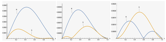
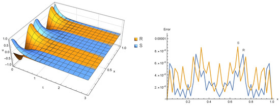
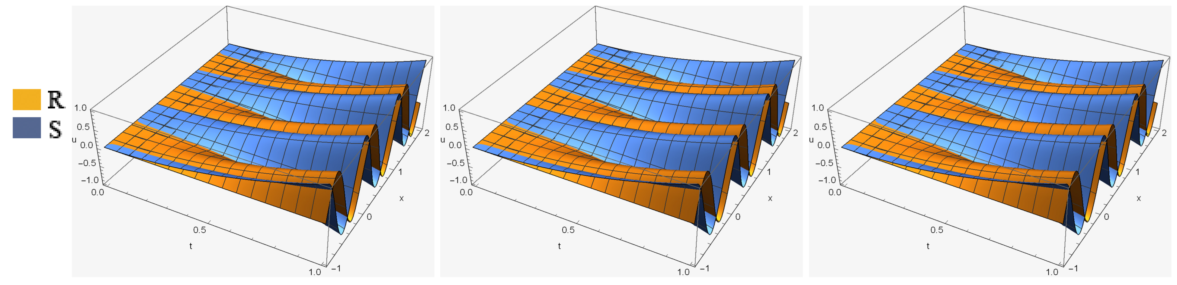
In Equation (1), we tested the efficiency and stability of the mentioned method by performing it for three different sets of parameters. For the first set, we chose $\alpha =0.1,0.3,0.5,0.7,0.9,$$\tau =0.002,$$N=40,t=1$ and $x\in [0,1]$ to compare with the previous papers [16,17,40]. Real $R\left(x,t\right)$ and imaginary $S\left(x,t\right)$ parts of a solution of $u\left(x,t\right)$, as well as $L_2$ and $L_{\infty }-$error norms (for the first set) from our method have been computed and listed in Table 2 and Table 3, respectively. As it shows, the error norms $L_2$ and $L_{\infty }$ got by our method are marginally less than the others. Approximate solutions of $R\left(x,t\right)$ and $S\left(x,t\right)$ are more accurate whenever the value of α decreases. Real $R\left(x,t\right)$ and imaginary $S\left(x,t\right)$ parts of solution of $u\left(x,t\right)$ (for the first set and $\alpha =0.1,0.5,0.9$) are demonstrate in Figure 1. Additionally, errors of $R\left(x,t\right)$ and $S\left(x,t\right)$ are shown in Figure 2.

Table 2. Error norms, numerical solutions and comparison of the exact solution of real part of Equation (1) for $\tau$ = 0.002, N = 40, a = 0, b = 1, T = 500, t = 1.

${\mathit{x}}_{\mathit{i}}$	$\mathit{\alpha }=0.1$	$\mathit{\alpha }=0.3$	$\mathit{\alpha }=$$0.5$	$\mathit{\alpha }=$$0.7$	$\mathit{\alpha }=0.9$	Exact
0.0	0.0	0.0	0.0	0.0	0.0	0.0
0.1	0.587719	0.587696	0.587634	0.587668	0.587586	0.587785
0.2	0.950943	0.9509	0.950776	0.950844	0.950677	0.951057
0.3	0.95093	0.950869	0.950694	0.95079	0.950548	0.951057
0.4	0.587683	0.58761	0.587399	0.587515	0.58722	0.587785
0.5	−0.000053	−0.000130	−0.000356	−0.000231	−0.000548	0.0
0.6	−0.587784	−0.587858	−0.588074	−0.587955	−0.588257	−0.587785
0.7	−0.951016	−0.951079	−0.951261	−0.95116	−0.951412	−0.951057
0.8	−0.951005	−0.951049	−0.951178	−0.951108	−0.951282	−0.951057
0.9	−0.58775	−0.587773	−0.587839	−0.587803	−0.587889	−0.587785
1.0	0.0	0.0	0.0	0.0	0.0	0.0
$L_{\infty }$	$1.2636\times {10}^{-4}$	$1.88153\times {10}^{-4}$	$2.74093\times {10}^{-4}$	$3.8663\times {10}^{-4}$	$5.67658\times {10}^{-4}$
$L_2$	$7.21151\times {10}^{-5}$	$1.10189\times {10}^{-4}$	$1.72782\times {10}^{-4}$	$2.55459\times {10}^{-4}$	$3.83777\times {10}^{-4}$

Table 3. Error norms, numerical solutions and comparison of the exact solution of imaginary part of Equation (1) for $\tau =0.002,N=40,a=0,b=1,T=500,t=1$.

${\mathit{x}}_{\mathit{i}}$	$\mathit{\alpha }=0.1$	$\mathit{\alpha }=0.3$	$\mathit{\alpha }=$$0.5$	$\mathit{\alpha }=0.7$	$\mathit{\alpha }=0.9$	Exact
0.0	1.0	1.0	1.0	1.0	1.0	1.0
0.1	0.809036	0.809022	0.808964	0.808999	0.808907	0.809017
0.2	0.309081	0.309056	0.308953	0.309015	0.308851	0.309017
0.3	−0.308895	−0.308926	−0.309056	−0.308978	−0.309182	−0.309017
0.4	−0.808847	−0.808879	−0.809015	−0.808933	−0.809143	−0.809017
0.5	−0.999809	−0.999838	−0.999962	−0.999887	−1.00007	−1.0
0.6	−0.808841	−0.808863	−0.808963	−0.808903	−0.809048	−0.809017
0.7	−0.308885	−0.308899	−0.308968	−0.308927	−0.309023	−0.309017
0.8	0.309092	0.309085	0.309044	0.309068	0.309016	0.309017
0.9	0.809043	0.80904	0.809022	0.809033	0.80901	0.809017
1.0	1.0	1.0	1.0	1.0	1.0	1.0
$L_{\infty }$	$1.91036\times {10}^{-4}$	$1.63543\times {10}^{-4}$	$1.17016\times {10}^{-4}$	$6.51301\times {10}^{-5}$	$1.71641\times {10}^{-4}$
$L_2$	$1.1824\times {10}^{-4}$	$9.9054\times {10}^{-5}$	$6.75574\times {10}^{-5}$	$3.99792\times {10}^{-5}$	$9.45488\times {10}^{-5}$

Figure 1. The computed approximation solutions of R and S in Equation (1) for $\alpha =0.9,\alpha =0.5,\alpha =0.1$, respectively, $\tau =0.002,a=0,b=1,N=40$ and $t=1$.

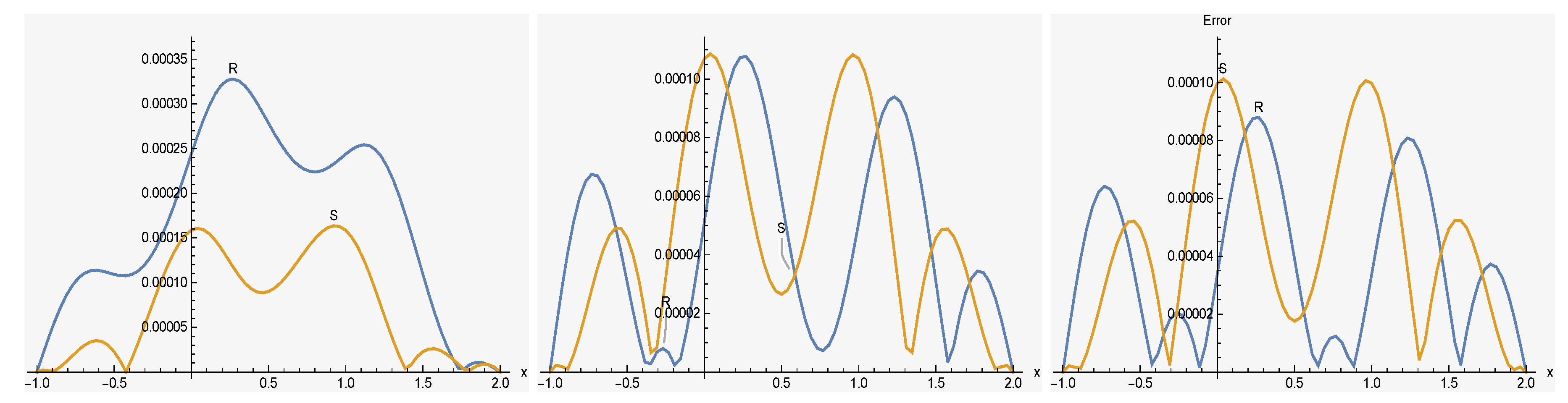
Figure 2. Error graph of R and S in Equation (1) for $\alpha =0.9,\alpha =0.5,\alpha =0.1$, respectively, $\tau =0.002,a=0,b=1,N=40andt=1$.

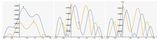
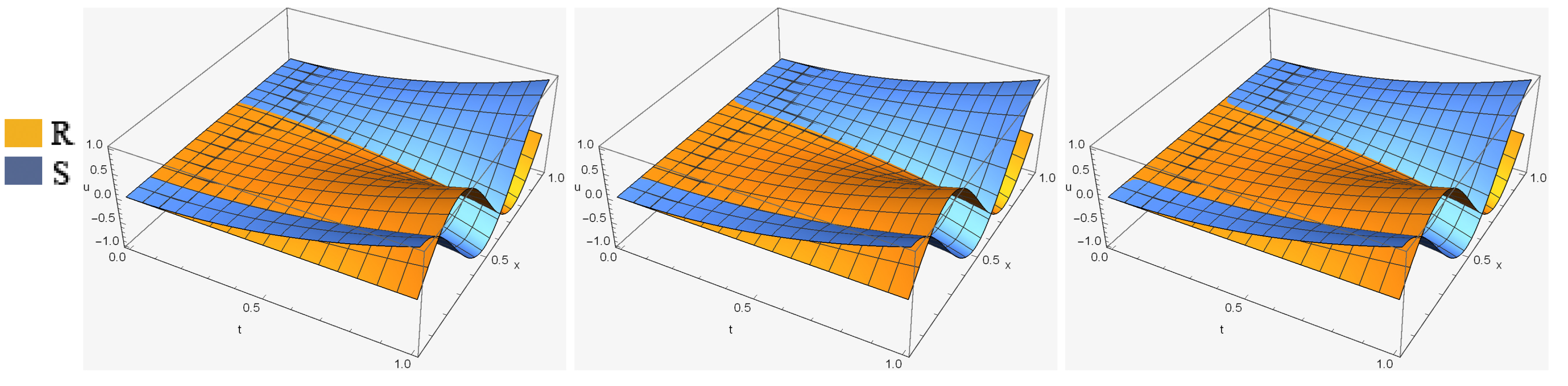
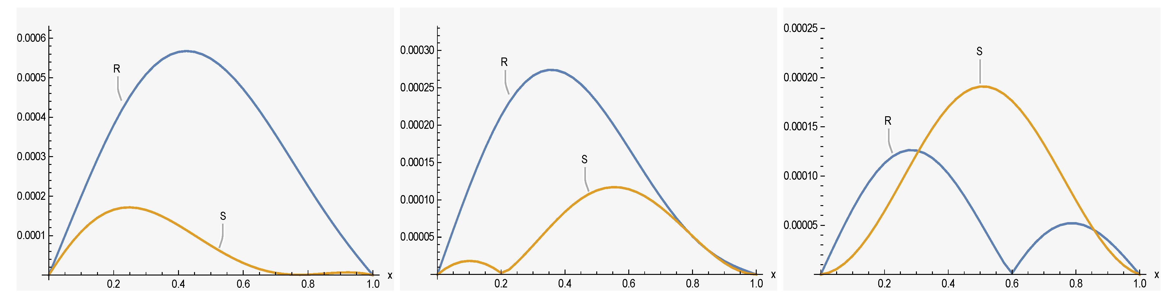
For the second set, we chose $\alpha =0.1,0.01,0.005,0.001,\tau =0.005,N=78,t=1$ and $x\in [-1,2].$ The $L_2$ and $L_{\infty }$− error norms of real $R\left(x,t\right)$ and imaginary $S\left(x,t\right)$ parts of a solution of $u\left(x,t\right)$ have been computed and listed in Table 4 and Table 5, respectively. In this set, we increase k and expand the region of the solution and by appropriate division, we got more accurate results, which are demonstrated in Figure 3. Additionally, error distributions of R and S are shown in Figure 4.

Table 4. Error norms of real part of Equation (1) for $\tau =0.005,N=78,a=-1,b=2,T=200,t=1$.

	$\mathit{\alpha }=0.1$	$\mathit{\alpha }=0.01$	$\mathit{\alpha }=0.005$	$\mathit{\alpha }=0.001$
$L_{\infty }$	$3.278811\times {10}^{-4}$	$1.07697\times {10}^{-4}$	$9.66734\times {10}^{-5}$	$8.79565\times {10}^{-5}$
$L_2$	$3.397343\times {10}^{-4}$	$9.57172\times {10}^{-5}$	$8.61773\times {10}^{-5}$	$7.93795\times {10}^{-5}$

Table 5. Error norms of imaginary part of Equation (1) for $\tau =0.005,$ N = 78, a = −1, b = 2, T = 200, t = 1.

	$\mathit{\alpha }=0.1$	$\mathit{\alpha }=0.01$	$\mathit{\alpha }=0.005$	$\mathit{\alpha }=0.001$
$L_{\infty }$	$1.63614\times {10}^{-4}$	$1.08568\times {10}^{-4}$	$1.04574\times {10}^{-4}$	$1.01291\times {10}^{-4}$
$L_2$	$1.613481\times {10}^{-4}$	$1.01424\times {10}^{-4}$	$9.76096\times {10}^{-5}$	$9.4623\times {10}^{-5}$

Figure 3. Computed approximation solutions of R and S in Equation (1) for $\alpha =0.1,\alpha =0.01,$$\alpha =0.001$, respectively, $\tau =0.005,a=-1,b=2,N=78$ and $t=1$.

Figure 4. Error graph of R and S in Equation (1) for $\alpha =0.1,\alpha =0.01,$$\alpha =0.001$, respectively, $\tau =0.005,a=-1,b=2,N=78andt=1$.

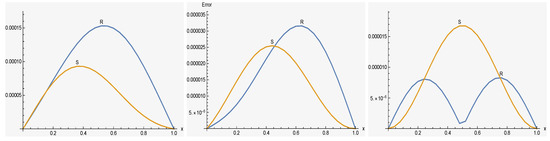
Finally, we tested the efficiency and stability of the chosen method by performing it for different values of $\alpha ,\tau ,N$, and region of solution. Thus, in the finally set, we took $\alpha =0.6,0.4,0.2,$$0.1,$$\tau =0.0025,N=25,t=0.5$ and $x\in [0,1].$ Numerical results of $R\left(x,t\right)$ and $S\left(x,t\right)$ of our proposed method, in addition to the the $L_2$ and $L_{\infty }-$error norms in solutions, are shown in Table 6 and Table 7, respectively. It is seen that while the value of α decreases, the numerical results become more accurate, we can clearly see this situation from the decreasing values of the $L_2$ and $L_{\infty }-$error norms. The accuracy of the numerical method is measured by computing the difference between the exact and numerical solutions at each point of division. As it is clear from the tables, the proposed algorithm gives better accuracy compared with the other. Graphs of numerical solutions and error distributions of R and S are presented in Figure 5 and Figure 6, respectively. Table 8 shows a comparison of the maximum absolute error for our results with the results in [40].

Table 6. Error norms, numerical solutions and comparison of the exact solution of real part of Equation (1) for $\tau =0.0025,N=25,a=0,b=1,T=200,t=0.5$.

${\mathit{x}}_{\mathit{i}}$	$\mathit{\alpha }=0.6$	$\mathit{\alpha }=0.4$	$\mathit{\alpha }=$$0.2$	$\mathit{\alpha }=0.1$	Exact
0.0	0.0	0.0	0.0	0.0	0.0
0.2	0.237691	0.237731	0.237757	0.237772	0.237764
0.4	0.146809	0.14688	0.146925	0.146951	0.146946
0.6	−0.147096	−0.147023	−0.146978	−0.146951	−0.146946
0.8	−0.237857	−0.237815	−0.237788	−0.237772	−0.237764
1.0	0.0	0.0	0.0	0.0	0.0
$L_{\infty }$	$1.53142\times {10}^{-4}$	$7.76316\times {10}^{-5}$	$3.15942\times {10}^{-5}$	$8.291928\times {10}^{-6}$
$L_2$	$1.04956\times {10}^{-4}$	$5.27316\times {10}^{-5}$	$2.0323\times {10}^{-5}$	$5.796502\times {10}^{-6}$

Table 7. Error norms, numerical solutions and comparison of the exact solution of imaginary part of Equation (1) for $\tau =0.0025,N=25,a=0,b=1,T=200,t=0.5$.

${\mathit{x}}_{\mathit{i}}$	$\mathit{\alpha }=0.6$	$\mathit{\alpha }=0.4$	$\mathit{\alpha }=$$0.2$	$\mathit{\alpha }=0.1$	Exact
0.0	0.25	0.25	0.25	0.25	0.25
0.2	0.0771853	0.077221	0.0772397	0.0772483	0.0772542
0.4	−0.202347	−0.202302	−0.202279	−0.202269	−0.202254
0.6	−0.202317	−0.202288	−0.202274	−0.202269	−0.202254
0.8	0.0772348	0.077244	0.0772479	0.0772484	0.0772542
1.0	0.25	0.25	0.25	0.25	0.25
$L_{\infty }$	$9.30703\times {10}^{-5}$	$4.82179\times {10}^{-5}$	$2.54937\times {10}^{-5}$	$1.67457\times {10}^{-5}$
$L_2$	$5.93658\times {10}^{-5}$	$3.06447\times {10}^{-5}$	$1.60645\times {10}^{-5}$	$1.03236\times {10}^{-5}$

Figure 5. Computed approximation solutions of R and S in Equation (1) for $\alpha =0.6,\alpha =0.2,\alpha =0.01$, respectively, $\tau =0.0025,a=0,b=1,N=40$ and $t=0.5$.

Figure 6. Error graph of R and S in Equation (1) for $\alpha =0.6,\alpha =0.2,\alpha =0.01$, respectively, $\tau =0.0025,a=0,b=1,N=25\mathrm{and}t=0.5$.

Table 8. Comparison of the error norms of real and imaginary parts in Equation (1) with Ref [40] for $\tau =1/512,\alpha =$$0.1$, $a=0,b=1$.

h	Trigonometric		Ref [40]
	Real Part	Imaginary Part	Real Part	Imaginary Part
1/4	6.83376$\times {10}^{-2}$	1.20244$\times {10}^{-1}$	4.2824$\times {10}^{-1}$	6.1227$\times {10}^{-1}$
1/9	1.37637$\times {10}^{-2}$	2.42034$\times {10}^{-2}$	7.0404$\times {10}^{-2}$	3.5194 $\times {10}^{-2}$
1/14	5.11408$\times {10}^{-3}$	9.04292$\times {10}^{-3}$	2.1873$\times {10}^{-2}$	1.4718$\times {10}^{-2}$
1/19	2.21103$\times {10}^{-3}$	3.84437$\times {10}^{-3}$	1.0022$\times {10}^{-2}$	7.1776$\times {10}^{-3}$
1/24	8.90286$\times {10}^{-4}$	1.54864$\times {10}^{-3}$	5.1958$\times {10}^{-3}$	3.8460$\times {10}^{-3}$
1/29	1.93239$\times {10}^{-4}$	3.21092$\times {10}^{-4}$	2.8536$\times {10}^{-3}$	2.1753$\times {10}^{-3}$
1/31	1.38283$\times {10}^{-5}$	1.247$\times {10}^{-5}$	−	−

Example 2.

In this example, we will consider the TFSE Equation (1) with initial-boundary conditions $u\left(x,0\right)=0,0\le x\le 1,$

$u(0,t)=0,u\left(1,t\right)=i{t}^2,t\ge 0,$ where

$$\begin{array}{c}\hfill f\left(x,t\right)=-\frac{2t^{2-\alpha }}{\Gamma (3-\alpha )}{x}^2-2t^2+t^6{x}^3(1-x)({(1-x)}^2+x^2)+i\left(\frac{\left(2t^{2-\alpha }\right)}{\Gamma (3-\alpha )}(1-x)x+t^6{x}^4\left(x^2+{(1-x)}^2\right)+2t^2\right).\end{array}$$

The exact solution of this problem is given by $u\left(x,t\right)=t^2\left((1-x)x+i{x}^2\right).$

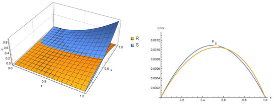
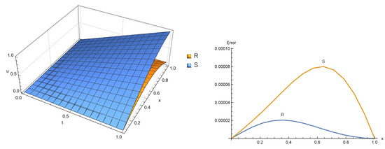
This example has been solved using the presented method with various values of $\tau ,$$\alpha =0.1,$$N=40,andt=1.$ Table 9 shows the numerical results based on maximum absolute errors acquired using the suggested approach for real and imaginary parts of the solution at $t=1$. Figure 7 illustrates the surface graph and curve of the absolute error of real and imaginary parts of the solution at $\tau =1/256, N=40,$ and $\alpha =0.1$.

Table 9. Error norms of real and imaginary parts of Equation (2) for different choices of $\tau$ at $N=40,$$\alpha =$$0.1$$,t=1$.

$\mathit{\tau }$	Real Part		Imaginary Part
	${\mathbf{L}}_{\infty }$	${\mathbf{L}}_{\mathbf{2}}$	${\mathbf{L}}_{\infty }$	${\mathbf{L}}_{\mathbf{2}}$
1/16	1.69582$\times {10}^{-2}$	1.23434$\times {10}^{-2}$	1.64917$\times {10}^{-2}$	6.1227$\times {10}^{-2}$
1/32	8.50622$\times {10}^{-3}$	6.19172$\times {10}^{-3}$	8.22627$\times {10}^{-3}$	6.09586$\times {10}^{-3}$
1/64	4.26873$\times {10}^{-3}$	3.10742$\times {10}^{-3}$	4.11967$\times {10}^{-3}$	3.0518$\times {10}^{-3}$
1/128	2.1514$\times {10}^{-3}$	1.56613$\times {10}^{-3}$	2.07201$\times {10}^{-3}$	1.5346$\times {10}^{-3}$
1/256	1.0934$\times {10}^{-3}$	7.95972$\times {10}^{-4}$	1.05034$\times {10}^{-3}$	7.77774$\times {10}^{-4}$
1/512	5.64571$\times {10}^{-4}$	4.11009$\times {10}^{-4}$	5.40111$\times {10}^{-4}$	3.99849$\times {10}^{-4}$

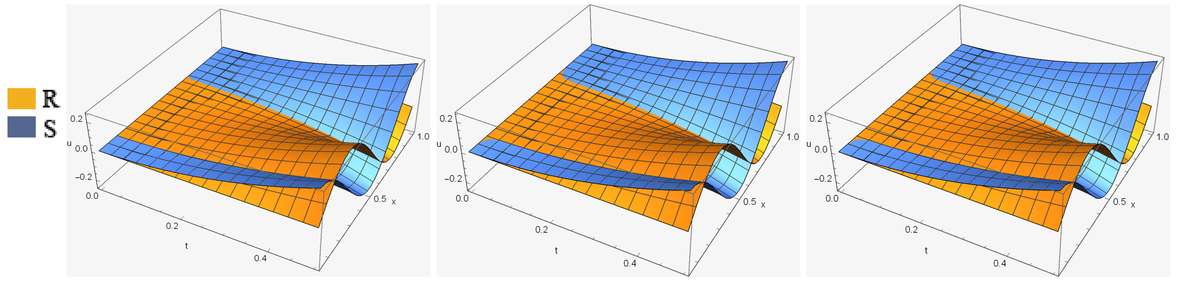
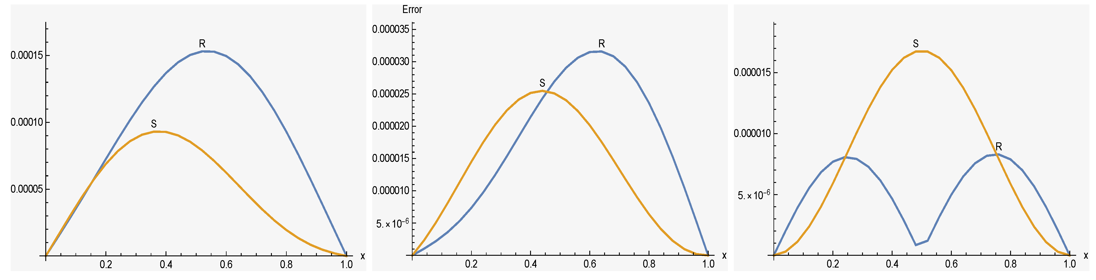
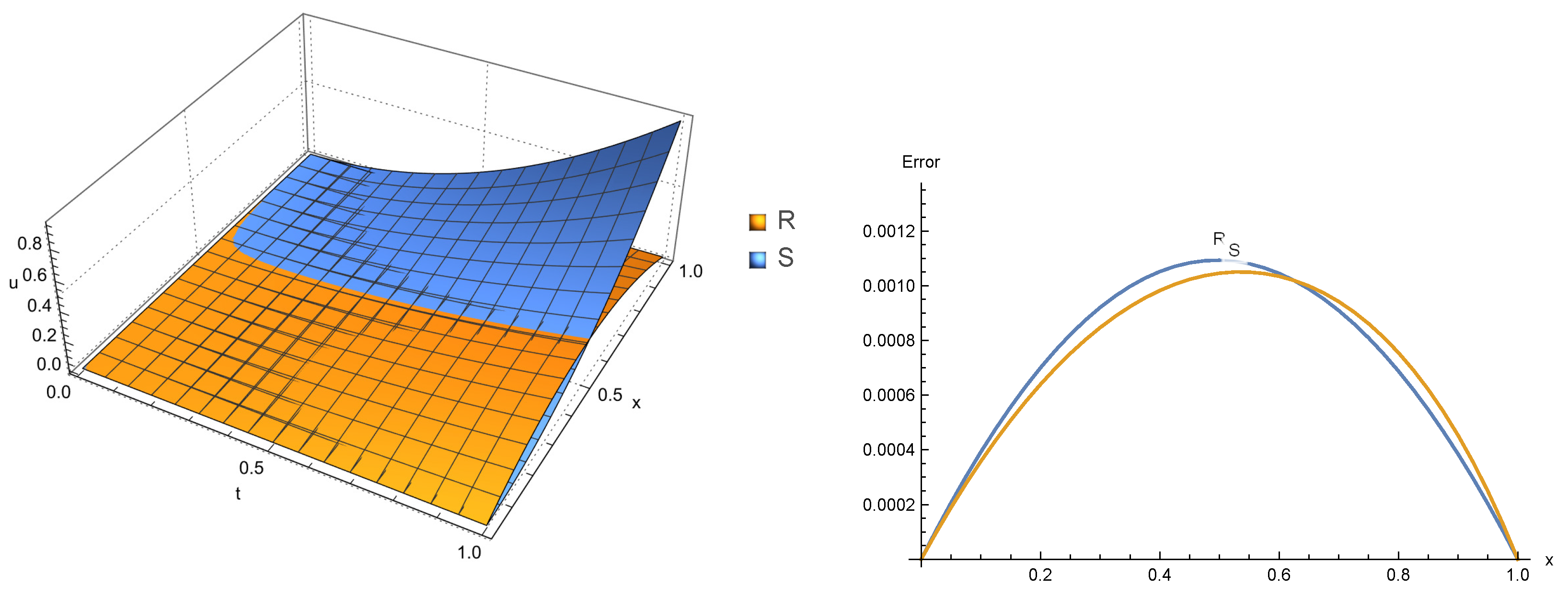
Figure 7. Computed approximation solutions and the error curves of R and S in Equation (2) for $\alpha =0.1\tau =1/256,a=0,b=1$, and $N=40$.

Example 3.

Consider fractional model of TFSE Equation(1) with initial-boundary conditions $u\left(x,0\right)=i{e}^{4i\pi x},0\le x\le 1,$

$u(0,t)=i{e}^{-4t},u\left(1,t\right)=i{e}^{4(\pi i-t)},t\ge 0,$ where

$$\begin{array}{c}\hfill f\left(x,t\right)=e^{4i\pi x}\left(\frac{{(-1)}^{\lceil \alpha \rceil }{4}^{\alpha }{e}^{i\pi \left(\lceil \alpha \rceil -\alpha \right)-4t}\Gamma (\lceil \alpha \rceil -\alpha ,-4t)}{\Gamma (\lceil \alpha \rceil -\alpha )}+i{e}^{-4t}\left(e^{-8t}-16{\pi }^2\right)\right),\end{array}$$

where $\lceil \alpha \rceil$ is a Ceiling function. The exact solution of this problem is given by $u\left(x,t\right)=i{e}^{4(i\pi x-t)}.$

Table 10 presented the $L_{\infty }$ and $L_2$ error norms for real and imaginary parts of the solution $u(x,t)$ for different choices of τ, $t=3,N=40,\alpha =0.5$ and $x\in [0,1]$. Figure 8 depicts the approximate solutions and error curves of absolute error obtained by the current approach for the real and imaginary sections of $u(x,t)$ for $\alpha =0.5$ at $N=40$ and $\tau =1/512$.

Table 10. Error norms of real and imaginary parts of Equation (3) for different choices of $\tau$ at $N=40,\alpha =0.5,t=3$.

$\mathit{\tau }$	Real Part		Imaginary Part
	${\mathbf{L}}_{\infty }$	${\mathbf{L}}_{\mathbf{2}}$	${\mathbf{L}}_{\infty }$	${\mathbf{L}}_{\mathbf{2}}$
1/16	1.43691$\times {10}^{-1}$	8.27474 $\times {10}^{-2}$	1.91429 $\times {10}^{-1}$	8.57523$\times {10}^{-2}$
1/32	5.55247 $\times {10}^{-2}$	3.11882$\times {10}^{-2}$	5.15378$\times {10}^{-2}$	2.64966 $\times {10}^{-2}$
1/64	9.35312 $\times {10}^{-3}$	4.66738$\times {10}^{-3}$	1.3519$\times {10}^{-2}$	7.51854$\times {10}^{-3}$
1/128	8.98237$\times {10}^{-4}$	4.9702$\times {10}^{-4}$	1.1515$\times {10}^{-3}$	6.62636 $\times {10}^{-4}$
1/256	7.5242$\times {10}^{-5}$	4.14215$\times {10}^{-5}$	1.28458$\times {10}^{-4}$	5.4835 $\times {10}^{-5}$
1/512	7.45923 $\times {10}^{-6}$	3.36356$\times {10}^{-6}$	8.6613$\times {10}^{-6}$	4.35745$\times {10}^{-6}$

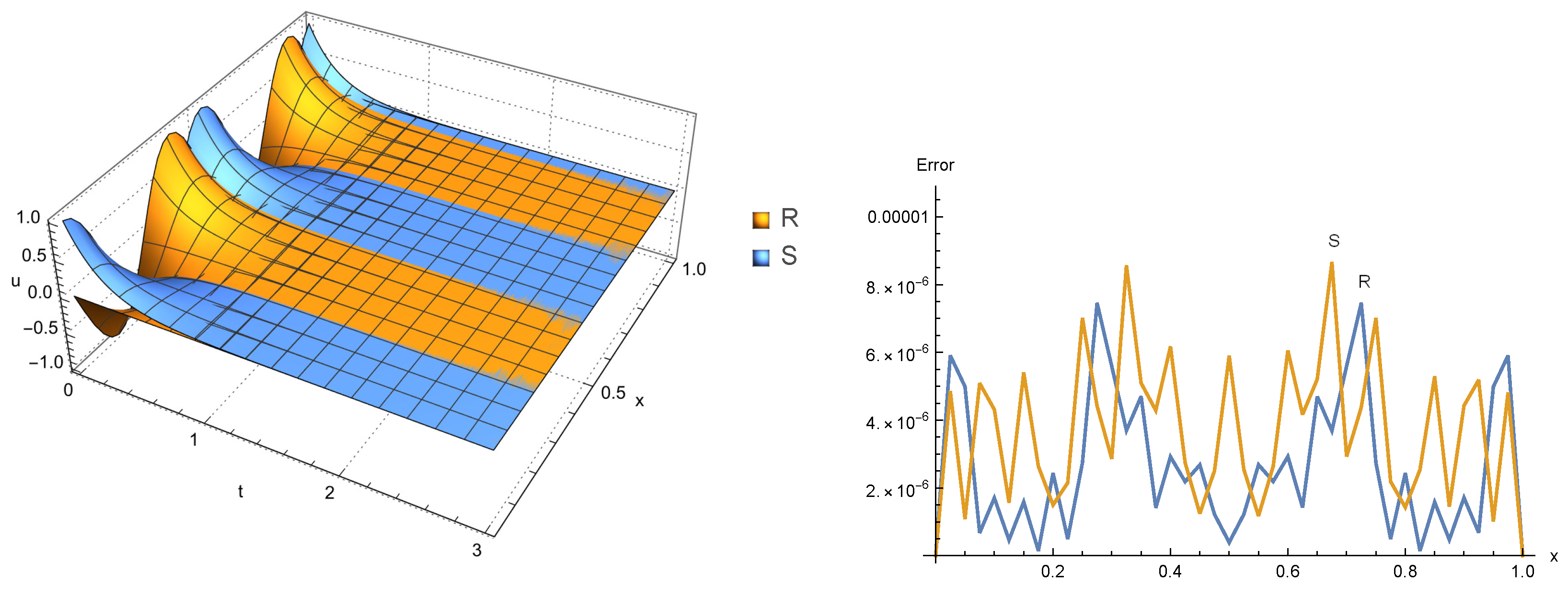
Figure 8. Computed approximation solutions and the error curves of R and S in Equation (3) for $\alpha =0.5\tau =1/512,a=0,b=1,$ and $N=40$.

Example 4.

To demonstrate that proposed technique may be applied to TFSE with non-local conditions, we consider the TFSE Equation (1) with the initial-boundary and non-local conditions

$u\left(x,0\right)=0,0\le x\le 1,$

$u(0,t)=0,{\int }_0^{1}u\left(x,t\right)=\frac{(-4+2\pi (1+i\left)\right)t}{{\pi }^2},t\ge 0,$ where,

$$\begin{array}{cc}\hfill f\left(x,t\right)=\left(xcos\left(\frac{\pi x}{2}\right)+isin\left(\frac{\pi x}{2}\right)\right)& \left(t^3\left(x^2{cos}^2\left(\frac{\pi x}{2}\right)+{sin}^2\left(\frac{\pi x}{2}\right)\right)+\frac{i{t}^{1-\alpha }}{\Gamma (2-\alpha )}\right)\hfill \\ & +t\left(-\frac{1}{4}i{\pi }^{2}sin\left(\frac{\pi x}{2}\right)-\pi sin\left(\frac{\pi x}{2}\right)-\frac{1}{4}{\pi }^{2}xcos\left(\frac{\pi x}{2}\right)\right)\hfill \end{array}$$

The exact solution of this problem is given by $u\left(x,t\right)=t\left(xcos\left(\frac{\pi x}{2}\right)+isin\left(\frac{\pi x}{2}\right)\right).$

we solved this example using the presented method with various choices of α at $N=15,$$\tau =1/512,$ and $t=1.$ Table 11 lists the $L_{\infty }$ and $L_2$ error norms for real and imaginary parts of $u(x,t)$. In case $\alpha =0.9$, we display the surface of real and imaginary parts of the approximate solution and the carves of of the absolute error in Figure 9.

Table 11. Error norms of real and imaginary parts of Equation (4) for different $\alpha$ at $N=15,\tau =1/512,$ and $t=1$.

$\mathit{\alpha }$	Real Part		Imaginary Part
	${\mathbf{L}}_{\infty }$	${\mathbf{L}}_{\mathbf{2}}$	${\mathbf{L}}_{\infty }$	${\mathbf{L}}_{\mathbf{2}}$
0.1	1.44004$\times {10}^{-5}$	8.26983$\times {10}^{-6}$	2.37462$\times {10}^{-5}$	1.34125$\times {10}^{-5}$
0.2	1.57166$\times {10}^{-5}$	7.33073$\times {10}^{-6}$	1.94386$\times {10}^{-5}$	1.29988$\times {10}^{-5}$
0.4	2.2306$\times {10}^{-5}$	1.34673$\times {10}^{-5}$	1.87377$\times {10}^{-5}$	1.18931$\times {10}^{-5}$
0.6	3.22106$\times {10}^{-5}$	2.15981$\times {10}^{-5}$	2.47268$\times {10}^{-5}$	1.39841$\times {10}^{-5}$
0.8	4.389 $\times {10}^{-5}$	3.00857 $\times {10}^{-5}$	3.12738 $\times {10}^{-5}$	1.7842$\times {10}^{-5}$
0.9	2.04375 $\times {10}^{-5}$	1.28792 $\times {10}^{-5}$	7.99336 $\times {10}^{-5}$	5.39379$\times {10}^{-5}$

Figure 9. Computed approximation solutions and the error curves of R and S in Equation (4) for $\alpha =0.9,\tau =1/512,a=0,b=1,N=15$ and $t=1$.

5. Conclusions

In this paper, we discussed an approximation technique for the numerical solution of the TFSE subject to initial-boundary conditions using cubic trigonometric B-splines. The fractional derivative was formulated with Caputo sense. The time derivative is discretized using the L1-approximate scheme, and a cubic trigonometric B-spline is used as an interpolating function in space with helping the Crank-Nicolson scheme. The stability analysis is proved by the Von Neumann approach. Comparing numerical results with exact solutions shows the applicability and efficiency of the proposed method. When the findings of the current approach are compared to those of [40] in Table 8, it is clear that the cubic trigonometric B-spline provides greater precision.

References

- Aksoy, A.; Irk, D.; Dag, I. Taylor collocation method for the numerical solution of the nonlinear Schrödinger equation using quintic B-spline basis. Phys. Wave Phenom. 2012, 20, 67–79. [Google Scholar] [CrossRef]
- Başhan, A. A mixed methods approach to Schrödinger equation: Finite difference method and quartic B-spline based differential quadrature method. Int. J. Optim. Control Theor. Appl. (IJOCTA) 2019, 9, 223–235. [Google Scholar] [CrossRef] [Green Version]
- Saka, B. A quintic B-spline finite-element method for solving the nonlinear Schrödinger equation. Phys. Wave Phenom. 2012, 20, 107–117. [Google Scholar] [CrossRef]
- Laskin, N. Fractional Schrödinger Equation. Phys. Rev. E 2002, 66, 056108. [Google Scholar] [CrossRef] [PubMed] [Green Version]
- Oldham, K.; Spanier, J. The Fractional Calculus Theory and Applications of Differentiation and Integration to Arbitrary Order; Elsevier: Amsterdam, The Netherlands, 1974. [Google Scholar]
- Podlubny, I. Fractional Differential Equations: An Introduction to Fractional Derivatives, Fractional Differential Equations, to Methods of Their Solution and Some of Their Applications; Elsevier: Amsterdam, The Netherlands, 1998. [Google Scholar]
- Hadhoud, A.R.; Srivastava, H.; Rageh, A.A. Non-polynomial B-spline and shifted Jacobi spectral collocation techniques to solve time-fractional nonlinear coupled Burgers’ equations numerically. Adv. Differ. Equ. 2021, 2021, 439. [Google Scholar] [CrossRef]
- Podlubny, I. Geometric and physical interpretation of fractional integration and fractional differentiation. arXiv 2001, 5, 367–386. [Google Scholar]
- Herzallah, M.A.; Gepreel, K.A. Approximate solution to the time–space fractional cubic nonlinear Schrodinger equation. Appl. Math. Model. 2012, 36, 5678–5685. [Google Scholar] [CrossRef]
- Hong, B.; Lu, D. Modified fractional variational iteration method for solving the generalized time-space fractional Schrödinger equation. Sci. World J. 2014, 2014, 964643. [Google Scholar] [CrossRef]
- Khan, N.A.; Jamil, M.; Ara, A. Approximate solutions to time-fractional Schrödinger equation via homotopy analysis method. Int. Sch. Res. Not. 2012, 2012, 197068. [Google Scholar] [CrossRef] [Green Version]
- Moa’ath, N.O.; El-Ajou, A.; Al-Zhour, Z.; Alkhasawneh, R.; Alrabaiah, H. Series solutions for nonlinear time-fractional Schrödinger equations: Comparisons between conformable and Caputo derivatives. Alex. Eng. J. 2020, 59, 2101–2114. [Google Scholar]
- Zhang, J.; Chen, H.; Sun, T.; Wang, J. Error analysis of a fully discrete scheme for time fractional Schrödinger equation with initial singularity. Int. J. Comput. Math. 2020, 97, 1636–1647. [Google Scholar] [CrossRef]
- Li, M.; Ding, X.; Xu, Q. Non-polynomial spline method for the time-fractional nonlinear Schrödinger equation. Adv. Differ. Equ. 2018, 2018, 318. [Google Scholar] [CrossRef]
- Liu, N.; Jiang, W. A numerical method for solving the time fractional Schrödinger equation. Adv. Comput. Math. 2018, 44, 1235–1248. [Google Scholar] [CrossRef]
- Esena, A.; Tasbozan, O. Numerical solution of time fractional nonlinear Schrodinger equation arising in quantum mechanics by cubic B-spline finite elements. Malaya J. Mat. (MJM) 2015, 3, 387–397. [Google Scholar]
- Esen, A.; Tasbozan, O. Numerical solution of time fractional Schrödinger equation by using quadratic B-spline finite elements. Ann. Math. Silesianae 2017, 31, 83–98. [Google Scholar] [CrossRef] [Green Version]
- Ran, M.; Zhang, C. Linearized Crank–Nicolson scheme for the nonlinear time–space fractional Schrödinger equations. J. Comput. Appl. Math. 2019, 355, 218–231. [Google Scholar] [CrossRef]
- Atangana, A.; Cloot, A.H. Stability and convergence of the space fractional variable-order Schrödinger equation. Adv. Differ. Equ. 2013, 2013, 80. [Google Scholar] [CrossRef] [Green Version]
- Wei, L.; He, Y.; Zhang, X.; Wang, S. Analysis of an implicit fully discrete local discontinuous Galerkin method for the timefractional Schrödinger equation. Finite Elem. Anal. Des. 2012, 59, 28–34. [Google Scholar] [CrossRef]
- Wei, L.; Zhang, X.; Kumar, S.; Yildirim, A. A numerical study based on an implicit fully discrete local discontinuous Galerkin method for the time-fractional coupled Schrödinger system. Comput. Math. Appl. 2012, 64, 2603–2615. [Google Scholar] [CrossRef] [Green Version]
- Yaseen, M.; Abbas, M.; Ismail, A.I.; Nazir, T. A cubic trigonometric B-spline collocation approach for the fractional sub-diffusion equations. Appl. Math. Comput. 2017, 293, 311–319. [Google Scholar] [CrossRef]
- Bhrawy, A.H.; Abdelkawy, M.A. A fully spectral collocation approximation for multi-dimensional fractional Schrödinger equations. J. Comput. Phys. 2015, 294, 462–483. [Google Scholar] [CrossRef]
- Tamsir, M.; Dhiman, N.; Srivastava, V.K. Cubic trigonometric B-spline differential quadrature method for numerical treatment of Fisher’s reaction-diffusion equations. Alex. Eng. J. 2018, 57, 2019–2026. [Google Scholar] [CrossRef]
- Heydari, M.; Atangana, A. A cardinal approach for nonlinear variable-order time fractional Schrödinger equation defined by Atangana-Baleanu–Caputo derivative. Chaos Solitons Fractals 2019, 128, 339–348. [Google Scholar] [CrossRef]
- Erfanian, M.; Zeidabadi, H.; Rashki, M.; Borzouei, H. Solving a nonlinear fractional Schrödinger equation using cubic B-splines. Adv. Differ. Equ. 2020, 2020, 1–20. [Google Scholar] [CrossRef]
- Zhang, H.; Jiang, X.; Wang, C.; Fan, W. Galerkin-Legendre spectral schemes for nonlinear space fractional Schrödinger equation. Numer. Algorithms 2018, 79, 337–356. [Google Scholar] [CrossRef]
- Wang, P.; Huang, C. An energy conservative difference scheme for the nonlinear fractional Schrödinger equations. J. Comput. Phys. 2015, 293, 238–251. [Google Scholar] [CrossRef]
- Zhang, Y.; Kumar, A.; Kumar, S.; Baleanu, D.; Yang, X.J. Residual power series method for time-fractional Schrödinger equations. J. Nonlinear Sci. Appl 2016, 9, 5821–5829. [Google Scholar] [CrossRef]
- Kaabar, M.K.; Martínez, F.; Gómez-Aguilar, J.F.; Ghanbari, B.; Kaplan, M.; Günerhan, H. New approximate analytical solutions for the nonlinear fractional Schrödinger equation with second-order spatio-temporal dispersion via double Laplace transform method. Math. Methods Appl. Sci. 2021, 44, 11138–11156. [Google Scholar] [CrossRef]
- Morales-Delgado, V.; Gómez-Aguilar, J.; Taneco-Hernández, M.; Baleanu, D. Modeling the fractional non-linear Schrödinger equation via Liouville–Caputo fractional derivative. Optik 2018, 162, 1–7. [Google Scholar] [CrossRef]
- Abdou, M.; Owyed, S.; Abdel-Aty, A.; Raffah, B.M.; Abdel-Khalek, S. Optical soliton solutions for a space-time fractional perturbed nonlinear Schrödinger equation arising in quantum physics. Results Phys. 2020, 16, 102895. [Google Scholar] [CrossRef]
- Chen, X.; Di, Y.; Duan, J.; Li, D. Linearized compact ADI schemes for nonlinear time-fractional Schrödinger equations. Appl. Math. Lett. 2018, 84, 160–167. [Google Scholar] [CrossRef]
- Mirzazadeh, M.; Akinyemi, L.; Şenol, M.; Hosseini, K. A variety of solitons to the sixth-order dispersive (3+1)-dimensional nonlinear time-fractional Schrödinger equation with cubic-quintic-septic nonlinearities. Optik 2021, 241, 166318. [Google Scholar] [CrossRef]
- Abdel-Salam, E.A.; Yousif, E.A.; El-Aasser, M.A. Analytical solution of the space-time fractional nonlinear Schrödinger equation. Rep. Math. Phys. 2016, 77, 19–34. [Google Scholar] [CrossRef]
- Raslan, K.; El-Danaf, T.S.; Ali, K.K. Collocation method with cubic trigonometric B-spline algorithm for solving coupled Burgers’ equations. Far East J. Appl. Math. 2016, 95, 109. [Google Scholar] [CrossRef]
- Murio, D.A. Implicit finite difference approximation for time fractional diffusion equations. Comput. Math. Appl. 2008, 56, 1138–1145. [Google Scholar] [CrossRef]
- El-Danaf, T.S.; Hadhoud, A.R. Parametric spline functions for the solution of the one time fractional Burgers’ equation. Appl. Math. Model. 2012, 36, 4557–4564. [Google Scholar] [CrossRef]
- Rubin, S.G.; Graves, R.A., Jr. A Cubic Spline Approximation for Problems in Fluid Mechanics; NASA STI/Recon Technical Report N; NASA: Washington, DC, USA, 1975; Volume 75, p. 33345. [Google Scholar]
- Mohebbi, A.; Abbaszadeh, M.; Dehghan, M. The use of a meshless technique based on collocation and radial basis functions for solving the time fractional nonlinear Schrödinger equation arising in quantum mechanics. Eng. Anal. Bound. Elem. 2013, 37, 475–485. [Google Scholar] [CrossRef]
Publisher’s Note: MDPI stays neutral with regard to jurisdictional claims in published maps and institutional affiliations. |
© 2022 by the authors. Licensee MDPI, Basel, Switzerland. This article is an open access article distributed under the terms and conditions of the Creative Commons Attribution (CC BY) license (https://creativecommons.org/licenses/by/4.0/).