1. Introduction
Learning stochastic processes is a fast growing research area in machine learning, as there is a considerable number of machine learning problems that involve the time variable as a component of datasets [
1,
2,
3,
4,
5]. Due to the nature of the time index, stochastic processes often possess “path features” [
6]. This additional information provided by the time index makes performing machine learning on stochastic processes quite different from other types of objects. Several new techniques are developed alongside studying such machine learning problems [
7,
8,
9,
10]. In this paper, we focus our study on a particular unsupervised learning problem: clustering of stochastic processes. Recently, clustering distribution stationary ergodic time series were motivated by and discussed in [
11,
12]. Later, Peng et al. [
13] developed Khaleghi et al. [
12]’s consistent clustering algorithms in order to cluster covariance stationary ergodic (discrete-time or continuous-time) stochastic processes. Please note that a distribution stationary ergodic stochastic process is not necessarily covariance stationary. Therefore, Peng et al. [
13] enlarged the class of stochastic processes for which one can apply the consistent clustering algorithms.
The motivation for this paper lies in the fact that assuming the observed data to follow a covariance stationary stochastic process seems still unrealistic. Our paper then tries to overcome this issue through developing a promising algorithm to cluster a more general class of stochastic processes, the so-called locally asymptotically self-similar processes. More precisely, the key path features of the observed stochastic processes are assumed to be known as Assumption 1 (see
Section 2). Compared to the stationarity, Assumption 1 is a much weaker constraint, for the reason that in many fields it was proved that the observed paths are sampled from functions (or functionals) of well-known locally asymptotically self-similar processes. For example, dynamics in financial markets (equity returns and interest rates) can be described based on geometric Brownian motions (gBm); long-term dependent or self-similar phenomena are often modeled by fractional Brownian motions (fBm) [
14]. The long-term financial indexes and curves, such as S&P 500, Dow Jones, NASDAQ, interest rates, VIX rates, and currency exchange rates can be modeled using multifractional Brownian motions (mBm) [
15,
16,
17,
18,
19,
20]. Modeling events using locally asymptotically self-similar processes can be widely found in other fields such as geology, biology, power, and energy [
21,
22]. Recently, there was growth of investigations on how to test and estimate locally asymptotically self-similar processes, and on how to apply machine learning analysis to such processes [
23,
24,
25,
26,
27,
28,
29,
30]. However, in as far as we know, there has not yet been a study on clustering locally asymptotically self-similar processes in the literature. Our paper then aims at shedding some light on clustering such processes.
Contrary to the conventional clustering of finite-dimensional data, clustering based on the paths’ features of the processes largely removes the noise by capturing the observations’ path features. Therefore, a nice dissimilarity measure should be the one that well characterizes the path features. In this context, “nice” refers to the property that the computational complexity and the prediction errors caused by the over-fitting issues are expected to be largely reduced. Moreover, with some path features, consistency of the clustering algorithm [
11,
12] may be obtained. Among all the stochastic process features, we focus on characterizing the property of ergodicity in this paper. However similar analysis can be made for other patterns of process features such as seasonality, Markov property and martingale property.
Ergodicity [
31] is a very typical feature possessed by several well-known processes, which is applied to financial time series analysis. It is tightly related to other process features, such as stationarity, long-term memory, and self-similarity [
32,
33]. In [
12,
13], it is shown that both distribution ergodicity and covariance ergodicity lead to obtaining an asymptotically consistent clustering algorithms for clustering processes. In this paper, we take one step further to relax the condition of ergodicity to the “local asymptotic ergodicity” [
34] and obtain the so-called “approximately asymptotically consistent algorithms” for clustering processes having such path property. This setting presents such a large class of processes that includes the well-known Lévy processes, some self-similar processes and some multifractional processes [
34].
Each clustering stochastic processes problem involves handling data, defining clusters, measuring dissimilarities, and finding groups efficiently; therefore, we organize the paper as follows.
Section 2 is devoted to introducing a class of locally asymptotically self-similar processes to which our clustering approaches apply. In
Section 3, a covariance-based dissimilarity measure is suggested and in
Section 4, the approximately asymptotically consistent algorithms for clustering both offline and online datasets are designed. A simulation study is performed in
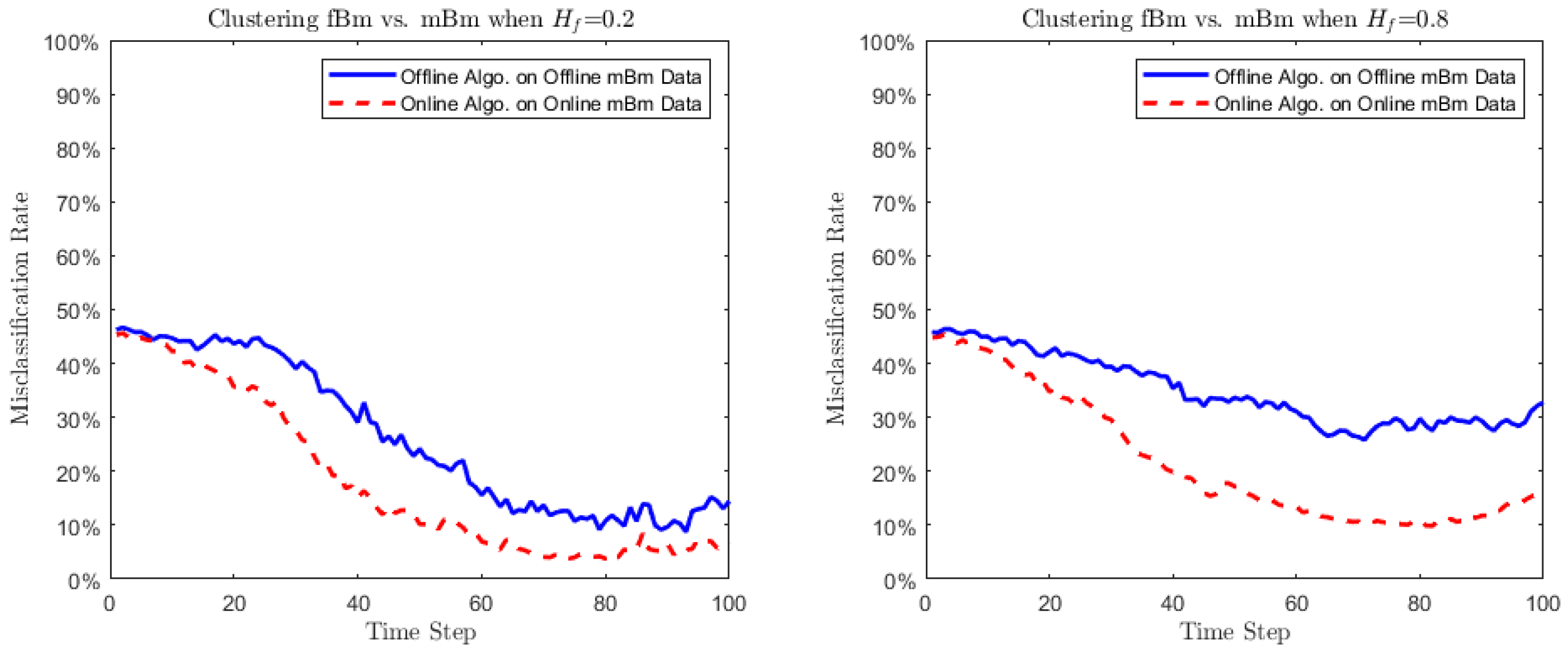
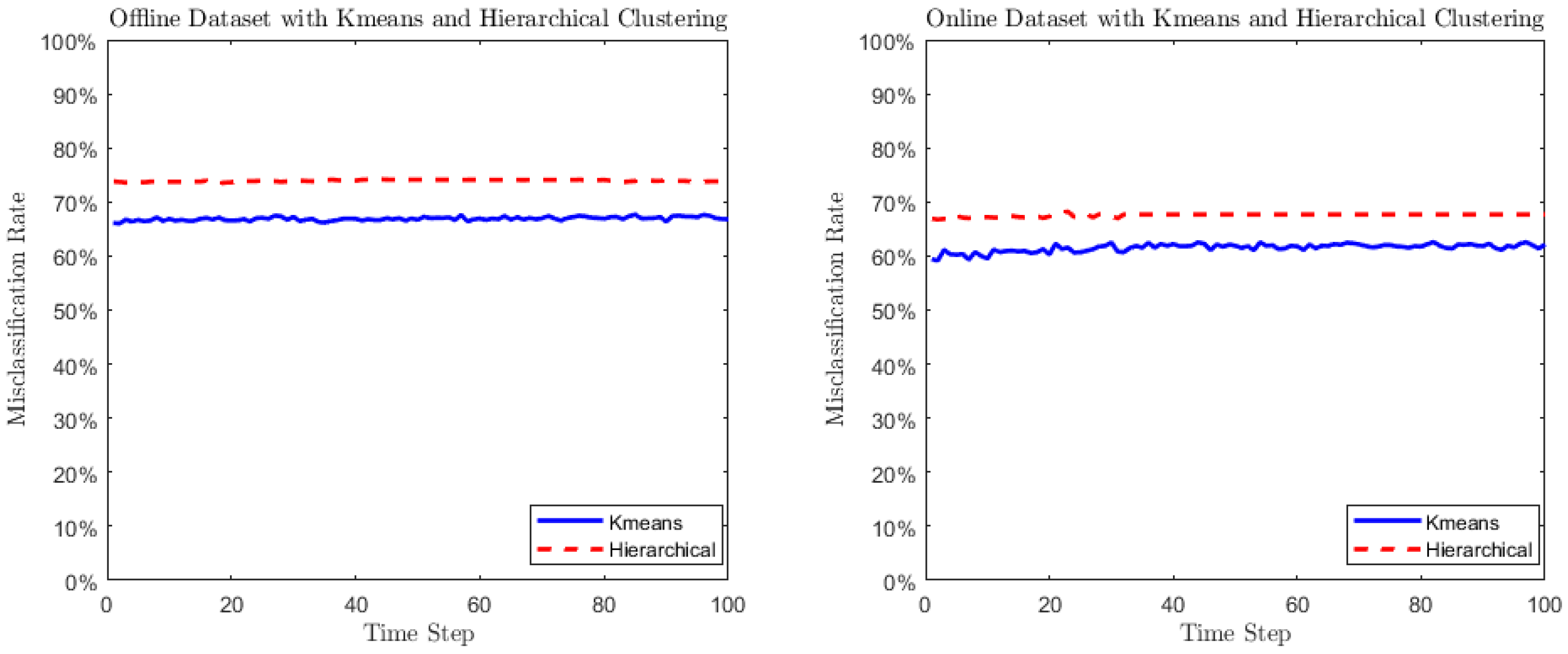
Section 5, where the algorithms are applied to cluster multifractional Brownian motions (mBm), an excellent representative of the class of locally asymptotically self-similar processes. In
Section 6, we perform cluster analysis over a global equity return data. Conventionally, stock returns of countries in the same region are considered to have similar patterns due to the common regional economic factors. However, recent empirical evidence shows that, as financial market globalization increases, global economic clusters switch from “geographical centriods” to “economic development centriods”. Our clustering algorithms show how “geography” and “economic development” jointly impact the equity returns of countries or regions. Considering the equities as stochastic processes in the clustering makes the analysis more promising. Finally,
Section 7 concludes and provides future prospects.
2. A Class of Locally Asymptotically Self-Similar Processes
Self-similar processes are a class of processes that are invariant in distribution under suitable scaling of time [
35,
36,
37]. These processes have been used to successfully model various time-scaling random phenomena observed in high frequency data, especially in the financial data and geological data.
Definition 1 (Self-similar process)
. A stochastic process (here the time indexes set is not necessarily continuous) is self-similar to self-similarity index if, for all , all and all ,where denotes the equality in joint probability distribution of two finite-dimensional random vectors. When
for
, it follows from (
1) that for any
,
Therefore taking
at both hand sides of (
2) yields
Self-similar processes are generally not distribution stationary but their increment processes can be distribution stationary (any finite subset’s joint distribution is invariant subject to time shift) or covariance stationary (its mean and covariance structure exist and are an invariant subject to time shift). From now on we restrict our setting to stochastically continuous-time self-similar processes only [
37]. i.e., a process
is stochastically continuous at
if
This assumption is weaker than the almost sure continuity. The process
is called (stochastically) continuous time over
if it is continuous at each
. For
, we call
the increment process (or simply the increments) of
. If a continuous-time self-similar process’ all increment processes are covariance stationary, its covariance structure can be explicitly given below:
Theorem 1. Let be a self-similar process with index and with covariance stationary increments. Then Theorem 1 can be obtained by replacing the distribution stationary increments assumption in Theorem 1.2 in [
36] with covariance stationary increments assumption. We briefly provide the proof below.
Proof. We first prove (
4). On one hand, using the fact that the increments of
are covariance stationary and (
3), we obtain
On the other hand, since
is self-similar to index
H, we have
Putting together (
6) and (
7) and the fact that
, we necessarily have
for all
. (
4) is proved.
For proving (
5) we first observe that, for
,
Next we can see from the facts that
is self-similar to index
H; that its increments are covariance stationary and (
4), that
The covariance stationarity yields
. (
5) then follows from (
8) and (
9). Theorem 1 is proved. □
We highlight that, contrary to Theorem 1.2 in [
36], the covariance stationary increment process of
in Theorem 1 is not necessarily distribution stationary. This fact inspires us to relax the distribution stationarity of the processes to the covariance stationarity in the forthcoming Assumption (
). Below, we introduce a natural extension of self-similar processes, the so-called locally asymptotically self-similar processes [
34,
38,
39].
Definition 2 (Locally asymptotically self-similar process)
. A continuous-time stochastic process with its index being a continuous function valued in , is called locally asymptotically self-similar, if for each , there exists a non-degenerate self-similar process with self-similarity index , such thatwhere the convergence is in the sense of all the finite-dimensional distributions. In (
10),
is called the
tangent process of
at
t [
38,
39]. Moreover, it is shown (see Theorem 3.8 in [
39]) that, if
is unique in law, it is then self-similar to index
and it has distribution stationary increments. Then the local asymptotic self-similarity generalizes the conventional self-similarity, in the sense that, any non-degenerate self-similar process with distribution stationary increments is locally asymptotically self-similar and its tangent process is itself. Furthermore, in a weaker sense, it is not difficult to show the following:
Proposition 1. Let be a continuous-time self-similar process with self-similarity index and with covariance stationary increments. Then all its tangent processes share the same mean and covariance function.
Proof. Since
is locally asymptotically self-similar, by definition at each
there exists a tangent process
such that
Next we show
s mean and covariance structure are uniquely determined.
Since
has covariance stationary increments, for any
,
, define the scaled increments
Again by the fact that
has covariance stationary increments, using (
4) in Theorem 1 we obtain
and by (
5) in Theorem 1, we have for
and
,
which does not depend on
.
It follows from (
11)–(
13) that
(
14) implies that all tangent processes of
possess zero-mean and equal covariance functions. By the way it is easy to derive from (
14) that these tangent processes have covariance stationary increments. Proposition 1 is proved. □
We remark from Proposition 1 that the tangent processes of may not be unique in law, but their finite-dimensional subsets have unique first and second order moments.
Based on the above discussion, throughout this paper, we assume that the observed datasets are sampled from a known number (denoted by ) of continuous-time processes satisfying the following condition:
Assumption 1. The processes are locally asymptotically self-similar; their tangent processes’ increment processes are autocovariance ergodic.
In Assumption 1, the autocovariance-ergodicity means that the sample autocovariance functions of the covariance stationary process converges in squared mean to the autocovariance functions of the process, i.e., a zero-mean (that is the case for the tangent processes’ increments) continuous-time process
is autocovariance ergodic if it is covariance stationary and satisfies
where
denotes the mean squared convergence:
. Please note that the above convergence (
15) yields
Thus, Assumption 1 says that the observed processes’ tangent processes have covariance stationary increments. The typical examples of locally asymptotically self-similar processes satisfying Assumption 1 are fractional Brownian motion (fBm) [
40], multifractional Brownian motion (mBm) [
41,
42,
43] and the generalized multifractional Brownian motion introduced in [
44]. Below, we focus our attention on mBm, which is used in our simulation study and real world application (see
Section 5 and
Section 6). MBm is a paradigmatic example of both multifractional stochastic processes and locally asymptotically self-similar processes. It naturally extends the classical fBm by allowing its Hurst parameter to vary with time. The mBm was introduced independently by Peltier and Lévy-Véhel [
41] and Benassi et al. [
42], using, respectively, integral moving average type representation and harmonizable integral representation of the fBm. These two types of mBms share several core features and their precise connection was studied by Stoev and Taqqu [
43], who show that the two types of mBms generally have different correlation structures. The most recent discussion on the definition of mBm is also made in [
43], where they define a general class of multifractional Gaussian processes which includes the above two types of mBms as two particular cases. In this paper, we adopt a definition of mBm through the so-called harmonizable integral representation (see (1.3) in [
43] or see [
42,
44]). Please note that our analysis and approaches are valid for all other versions of mBms in the literature.
Definition 3 (Multifractional Brownian motion)
. A multifractional Brownian motion is a continuous-time Gaussian process defined by:where: denotes a complex-valued Gaussian measure (see Proposition 2.1 in [43]) satisfying with being the Fourier transform of f and being a standard Brownian motion.
The Hurst functional parameter is a Hölder function with exponent . Subject to this constraint the paths of mBm are almost surely continuous functions.
Theorem 4.1 in [
43] gives the covariance function of
: for
,
where
It is known that the pointwise Hölder exponent (pHe) of
is almost surely equal to
at each
t [
42]. Recall that, for a continuous-time nowhere differentiable process
, its local Hölder regularity can be measured by the pHe
defined by: for each
,
For a continuous but undifferentiable function, the pHe measures its “local roughness”: the smaller the pHe is at time
t, the more “fractals” should be observed around
t in the path. When
becomes a constant, mBm reduces to an fBm with Hurst parameter equal to
H. More generally, it can be seen from [
34] that mBm is locally asymptotically self-similar satisfying Assumption 1. Its tangent process at each
t is an fBm
with index
:
where
is a deterministic function only depending on
. In the literature, some studies are particularly focused on the statistical inference problems around the pHe of processes and their applications. This study is motivated by modeling using locally asymptotically self-similar processes as well. We refer the readers to [
45,
46,
47,
48,
49,
50].
As one of the most natural extensions of fBm, mBm has, at present, broad applications. Unlike fBm, mBm allows its Hurst parameter H to change with time. This allows us to model different regimes of the stochastic process with one single model. For example, during a financial crisis, asset volatility may rise significantly, while it is much lower in the peaceful period. Likewise, empirical evidence shows that there have been periods of different volatilities in either exchange rates or interest rates. An fBm (or a self-similar process) is unable to capture the above phenomena. This motivates researchers to introduce mBm into finance as an alternative or improvement of fBm.
The assumption of covariance stationarity inspires us to introduce a covariance-based dissimilarity measure between the sample paths, in order to capture the level of differences between the two corresponding covariance stationary processes. Later we show that the assumption of autocovariance-ergodicity is sufficient for the clustering algorithms to be approximately asymptotically consistent.


