Boundary Layer via Multifractal Mass Conductivity through Remote Sensing Data in Atmospheric Dynamics

Abstract

In this manuscript, multifractal theories of motion based on scale relativity theory are considered in the description of atmospheric dynamics. It is shown that these theories have the potential to highlight nondimensional mass conduction laws that describe the propagation of atmospheric entities. Then, using special operational procedures and harmonic mappings, these equations can be rewritten and simplified for their plotting and analysis to be performed. The inhomogeneity of these conduction phenomena is analyzed, and it is found that it can fluctuate and increase at certain fractal dimensions, leading to the conclusion that certain atmospheric structures and phenomena of either atmospheric transmission or stability can be explained by atmospheric fractal dimension inversions. Finally, this hypothesis is verified using ceilometer data throughout the atmospheric profiles.

1. Introduction

Often, to describe atmospheric dynamics, models must be constructed with combinations of physical theories and computer simulation [1,2,3,4,5]. If such descriptions imply simulations based on specific algorithms, this development in relation to physical theories relies on two classes of models [4,5,6,7]:

(i)

Based on typical conservation laws developed on integer-dimensional spaces, also known as differentiable models [1,2,3];

(ii)

Based on conservation laws developed on non-integer-dimensional spaces, or non-differentiable models (fractal or multifractal) [6,7].

It is a recent development that new models based on Scale Relativity Theory have appeared, either using monofractal dynamics or multifractal dynamics, as with the Multifractal Theory of Motion [8,9,10]. In both situations, presupposing that the atmosphere is both structurally and functionally assimilated to multifractal objects, atmospheric dynamics can be described through the motions of such multifractal structural units on continuous and non-differentiable curves, also known as multifractal curves. Because, for a large temporal scale resolution, with respect to the inverse of the highest Lyapunov exponent trajectories, these structural units can be replaced with collections of potential trajectories; it is then possible to replace the notion of “deterministic definite trajectory” with that of a probability density [11,12].

2. Hydrodynamic Multifractal Scenario Conservation Laws

In the description of complex system dynamics through a hydrodynamic multifractal scenario, it is possible to find the involvement of the specific multifractal impulse conservation law [13,14]:

$${\partial }_{\mathrm{t}}{\mathrm{v}}^{\mathrm{i}}+{\mathrm{v}}^{\mathrm{l}}{\partial }_{\mathrm{l}}{\mathrm{v}}^{\mathrm{i}}=-{\partial }^{\mathrm{i}}\mathrm{Q}, \mathrm{i}=1,2,3$$

(1)

and that of the conservation law of the multifractal states density:

$${\partial }_{\mathrm{t}}\mathsf{\rho }+{\partial }^{\mathrm{l}}\left({\mathsf{\rho }\mathrm{v}}^{\mathrm{l}}\right)=0$$

(2)

where:

$$\begin{array}{l}{\partial }_{\mathrm{t}}=\frac{\partial }{\partial \mathrm{t}},{\partial }_{\mathrm{l}}=\frac{\partial }{\partial {\mathrm{x}}^{\mathrm{l}}}\\ \mathsf{\rho }=\mathsf{\psi }\overline{\mathsf{\psi }}, \mathsf{\psi }=\sqrt{\mathsf{\rho }}{\mathrm{e}}^{\mathrm{is}}\\ \mathrm{Q}=2{\mathsf{\lambda }}^2{\left(\mathrm{dt}\right)}^{\left[\frac{4}{\mathrm{f}\left(\mathsf{\alpha }\right)}\right]-2}\frac{{\partial }_{\mathrm{l}}{\partial }^{\mathrm{l}}\sqrt{\mathsf{\rho }}}{\sqrt{\mathsf{\rho }}}=\frac{{\mathrm{u}}_{\mathrm{i}}{\mathrm{u}}^{\mathrm{i}}}{2}+\mathsf{\lambda }{\left(\mathrm{dt}\right)}^{\left[\frac{2}{\mathrm{f}\left(\mathsf{\alpha }\right)}\right]-1}{\partial }^{\mathrm{l}}{\mathrm{u}}_{\mathrm{l}}\\ {\partial }_{\mathrm{t}}\mathsf{\rho }+{\partial }_{\mathrm{x}}\left(\mathsf{\rho }\mathrm{v}\right)=0\end{array}$$

(3)

In the above relations, the given measures have the following physical meanings:

-

t is nonmultifractal time, an affine parameter of movement curves of the entities found in the complex system;

-

x^l is the multifractal spatial coordinate;

-

vⁱ is the velocity field at a differentiable scale resolution;

-

uⁱ is the velocity field at a non-differentiable scale resolution;

-

dt is the scale resolution;

-

λ is a constant coefficient associated with the multifractal-nonmultifractal scale transition;

-

ρ is the state density;

-

ψ is the state function with the amplitude $\sqrt{\mathsf{\rho }}$ and phase s;

-

Q is the scalar specific multifractal potential which quantifies the multifractalization degree of the movement curves in the complex system;

-

f(α) is the singularity spectrum of order α = α(D_F) where D_F is the fractal dimension of movement curves of the complex system entities. This spectrum allows the identification of universality classes in the complex system dynamics, even when attractors have different aspects, and it also allows the identification of areas in which the dynamics can be characterized by a specific fractal dimension.

Because of its nonlinearity, Equations (1) and (2) admit analytical solutions only in special, particular cases. Such a case is dictated by the one-dimensional dynamics of the complex system entities through the following:

$$\begin{gathered} {\partial }_{\mathrm{t}}\mathrm{v}+\mathrm{v}{\partial }_{\mathrm{x}}\mathrm{v}=2{\mathsf{\lambda }}^2{\left(\mathrm{dt}\right)}^{\left[\frac{4}{\mathrm{f}\left(\mathsf{\alpha }\right)}\right]-2}\frac{{\partial }_{\mathrm{xx}}\sqrt{\mathsf{\rho }}}{\sqrt{\mathsf{\rho }}} \\ {\partial }_{\mathrm{t}}\mathsf{\rho }+{\partial }_{\mathrm{x}}\left(\mathsf{\rho }\mathrm{v}\right)=0 \end{gathered}$$

(4)

with the initial and boundary constraints:

$$\begin{gathered} \mathrm{v}\left(\mathrm{x},\mathrm{t}=0\right)={\mathrm{v}}_0, \mathsf{\rho }\left(\mathrm{x},\mathrm{t}=0\right)={\mathsf{\rho }}_0{\mathrm{e}}^{-{\left(\frac{\mathrm{x}}{\mathrm{a}}\right)}^2} \\ \mathrm{v}\left(\mathrm{x}=\mathrm{ct},\mathrm{t}\right)={\mathrm{v}}_0, \mathsf{\rho }\left(\mathrm{x}=-\infty ,\mathrm{t}\right)=\mathsf{\rho }\left(\mathrm{x}=+\infty ,\mathrm{t}\right)=0 \end{gathered}$$

(5)

The following solution is found:

$$\frac{{\mathrm{v}}_0{\mathrm{a}}^2+{\left[\frac{\mathsf{\lambda }{\left(\mathrm{dt}\right)}^{\left[\frac{2}{\mathrm{f}\left(\mathsf{\alpha }\right)}\right]-1}}{\mathrm{a}}\right]}^2\mathrm{xt}}{{\mathrm{a}}^2+{\left[\frac{\mathsf{\lambda }{\left(\mathrm{dt}\right)}^{\left[\frac{2}{\mathrm{f}\left(\mathsf{\alpha }\right)}\right]-1}}{\mathrm{a}}\mathrm{t}\right]}^2}$$

(6)

and:

$$\mathsf{\rho }=\frac{{\mathsf{\pi }}^{-\frac{1}{2}}}{{\left\{{\mathrm{a}}^2+{\left[\frac{\mathsf{\lambda }{\left(\mathrm{dt}\right)}^{\left[\frac{2}{\mathrm{f}\left(\mathsf{\alpha }\right)}\right]-1}}{\mathrm{a}}\mathrm{t}\right]}^2\right\}}^{\frac{1}{2}}}·{\mathrm{e}}^{\left\{-\frac{{\left(\mathrm{x}-{\mathrm{v}}_0\mathrm{t}\right)}^2}{{\mathrm{a}}^2+{\left[\frac{\mathsf{\lambda }{\left(\mathrm{dt}\right)}^{\left[\frac{2}{\mathrm{f}\left(\mathsf{\alpha }\right)}\right]-1}}{\mathrm{a}}\mathrm{t}\right]}^2}\right\}}$$

(7)

This solution, through the nondimensional variables is:

$$\frac{\mathrm{v}}{{\mathrm{v}}_0}=\overline{\mathrm{v}}, \mathsf{\rho }\sqrt{\mathsf{\pi }}\mathrm{a}=\overline{ \mathsf{\rho }}, \frac{\mathrm{x}}{{\mathrm{v}}_0\mathsf{\tau }}=\mathsf{\xi }, \frac{\mathrm{t}}{\mathsf{\tau }}=\mathsf{\eta }$$

(8)

and through the nondimensional parameters,

$$\mathsf{\theta }=\frac{\mathsf{\lambda }{\left(\mathrm{dt}\right)}^{\left[\frac{2}{\mathrm{f}\left(\mathsf{\alpha }\right)}\right]-1}\mathsf{\tau }}{{\mathrm{a}}^2}, \mathsf{\mu }=\frac{{\mathrm{v}}_0\mathsf{\tau }}{\mathrm{a}}$$

(9)

can be rewritten as:

$$\overline{\mathrm{v}}=\frac{1+{\mathsf{\theta }}^2\mathsf{\xi }\mathsf{\eta }}{1+{\mathsf{\theta }}^2{\mathsf{\eta }}^2}$$

(10)

and:

$$\overline{\mathsf{\rho }}=\frac{1}{\sqrt{1+{\mathsf{\theta }}^2{\mathsf{\eta }}^2}}·{\mathrm{e}}^{\left[-{\mathsf{\mu }}^2\frac{{\left(\mathsf{\xi }-\mathsf{\eta }\right)}^2}{1+{\mathsf{\theta }}^2{\mathsf{\eta }}^2}\right]}$$

(11)

Through Equation (3), the solutions in Equations (6) and (7) allow us to construct the following set of variables:

-

The velocity field at a non-differentiable scale:

$$\mathrm{u}=2\mathsf{\lambda }{\left(\mathrm{dt}\right)}^{\left[\frac{2}{\mathrm{f}\left(\mathsf{\alpha }\right)}\right]-1}·\frac{\left(\mathrm{x}-{\mathrm{v}}_0\mathrm{t}\right)}{{\mathrm{a}}^2+{\left[\frac{\mathsf{\lambda }{\left(\mathrm{dt}\right)}^{\left[\frac{2}{\mathrm{f}\left(\mathsf{\alpha }\right)}\right]-1}}{\mathrm{a}}\mathrm{t}\right]}^2}$$

(12)

-

The specific multifractal force field:

$$\mathrm{f}=-{\partial }_{\mathrm{x}}\mathrm{Q}=2\mathsf{\lambda }{\left(\mathrm{dt}\right)}^{\left[\frac{4}{\mathrm{f}\left(\mathsf{\alpha }\right)}\right]-2}·\frac{\left(\mathrm{x}-{\mathrm{v}}_0\mathrm{t}\right)}{{\left\{{\mathrm{a}}^2+{\left[\frac{\mathsf{\lambda }{\left(\mathrm{dt}\right)}^{\left[\frac{2}{\mathrm{f}\left(\mathsf{\alpha }\right)}\right]-1}}{\mathrm{a}}\mathrm{t}\right]}^2\right\}}^2}$$

(13)

This set of variables employs the notations:

$$\frac{\mathrm{u}}{2{\mathrm{v}}_0}=\overline{\mathrm{u}}, \frac{\mathrm{f}\mathsf{\tau }}{2{\mathrm{v}}_0}=\overline{\mathrm{f}}$$

(14)

Considering Equations (8) and (9) they become:

$$\overline{\mathrm{u}}=\mathsf{\theta }\frac{\mathsf{\xi }-\mathsf{\eta }}{1+{\mathsf{\theta }}^2{\mathsf{\eta }}^2}$$

(15)

respectively:

$$\overline{\mathrm{f}}={\mathsf{\theta }}^2\frac{\mathsf{\xi }-\mathsf{\eta }}{{\left(1+{\mathsf{\theta }}^2{\mathsf{\eta }}^2\right)}^2}$$

(16)

Then, let us assume the functionality, in nondimensional coordinates, of a relation of the form:

$$\overline{\mathrm{j}}=\overline{\mathsf{\sigma }}\overline{\mathrm{f}}$$

(17)

where $\overline{\mathrm{j}}$ is a mass current density, $\overline{\mathrm{f}}$ is the nondimensional specific multifractal force field, and $\overline{\mathsf{\sigma }}$ is a mass conductivity, which then allows us to define the following conductivity types:

-

Conductivity at differentiable scale resolutions:

$$\overline{{\mathsf{\sigma }}_{\mathrm{D}}}=\frac{\overline{\mathsf{\rho }}\overline{\mathrm{v}}}{\overline{\mathrm{f}}}=\sqrt{1+{\mathsf{\theta }}^2{\mathsf{\eta }}^2}\frac{1+{\mathsf{\theta }}^2\mathsf{\xi }\mathsf{\eta }}{{\mathsf{\theta }}^2\left(\mathsf{\xi }-\mathsf{\eta }\right)}{\mathrm{e}}^{\left[-{\mathsf{\mu }}^2\frac{{\left(\mathsf{\xi }-\mathsf{\eta }\right)}^2}{1+{\mathsf{\theta }}^2{\mathsf{\eta }}^2}\right]}$$

(18)

-

Conductivity at non-differentiable scale resolutions:

$$\overline{{\mathsf{\sigma }}_{\mathrm{F}}}=\frac{\overline{\mathsf{\rho }}\overline{\mathrm{u}}}{\overline{\mathrm{f}}}=\sqrt{1+{\mathsf{\theta }}^2{\mathsf{\eta }}^2}{\left(\frac{\mathsf{\mu }}{\mathsf{\theta }}\right)}^2{\mathrm{e}}^{\left[-{\mathsf{\mu }}^2\frac{{\left(\mathsf{\xi }-\mathsf{\eta }\right)}^2}{1+{\mathsf{\theta }}^2{\mathsf{\eta }}^2}\right]}$$

(19)

-

Conductivity at global scale resolutions:

$$\overline{\mathsf{\sigma }}=\frac{\overline{\mathsf{\rho }}\left(\overline{\mathrm{v}}+\mathrm{i}\overline{\mathrm{u}}\right)}{\mathrm{f}}=\overline{{\mathsf{\sigma }}_{\mathrm{D}}}+\mathrm{i}\overline{{\mathsf{\sigma }}_{\mathrm{F}}}=\sqrt{1+{\mathsf{\theta }}^2{\mathsf{\eta }}^2}\left[\frac{1+{\mathsf{\theta }}^2\mathsf{\xi }\mathsf{\eta }}{{\mathsf{\theta }}^2\left(\mathsf{\xi }-\mathsf{\eta }\right)}+\mathrm{i}{\left(\frac{\mathsf{\mu }}{\mathsf{\theta }}\right)}^2\right]{\mathrm{e}}^{\left[-{\mathsf{\mu }}^2\frac{{\left(\mathsf{\xi }-\mathsf{\eta }\right)}^2}{1+{\mathsf{\theta }}^2{\mathsf{\eta }}^2}\right]}$$

(20)

In this context, since the $\mathsf{\theta }$ parameter is a measure of the multifractality degree, then $\mathsf{\epsilon }=\frac{1}{\mathsf{\theta }}$ will function as a measure of an ordering degree. Then, the conductivity species in Equations (18)–(20) change as:

-

Conductivity at differentiable scale resolutions:

$$\overline{{\mathsf{\sigma }}_{\mathrm{D}}}=\sqrt{{\mathsf{\epsilon }}^2+{\mathsf{\eta }}^2}\frac{{\mathsf{\epsilon }}^2+\mathsf{\xi }\mathsf{\eta }}{\mathsf{\epsilon }\left(\mathsf{\xi }-\mathsf{\eta }\right)}{\mathrm{e}}^{\left[-{\left(\mathsf{\mu }\mathsf{\epsilon }\right)}^2\frac{{\left(\mathsf{\xi }-\mathsf{\eta }\right)}^2}{{\mathsf{\epsilon }}^2+{\mathsf{\eta }}^2}\right]}$$

(21)

-

Conductivity at non-differentiable scale resolutions:

$$\overline{{\mathsf{\sigma }}_{\mathrm{F}}}=\sqrt{{\mathsf{\epsilon }}^2+{\mathsf{\eta }}^2}{\mathsf{\epsilon }\mathsf{\mu }}^2{\mathrm{e}}^{\left[-{\left(\mathsf{\mu }\mathsf{\epsilon }\right)}^2\frac{{\left(\mathsf{\xi }-\mathsf{\eta }\right)}^2}{{\mathsf{\epsilon }}^2+{\mathsf{\eta }}^2}\right]}$$

(22)

-

Conductivity at global scale resolutions:

$$\overline{\mathsf{\sigma }}=\sqrt{{\mathsf{\epsilon }}^2+{\mathsf{\eta }}^2}\left[\frac{{\mathsf{\epsilon }}^2+\mathsf{\xi }\mathsf{\eta }}{\mathsf{\epsilon }\left(\mathsf{\xi }-\mathsf{\eta }\right)}+{\mathrm{i}\mathsf{\epsilon }\mathsf{\mu }}^2\right]{\mathrm{e}}^{\left[-{\left(\mathsf{\mu }\mathsf{\epsilon }\right)}^2\frac{{\left(\mathsf{\xi }-\mathsf{\eta }\right)}^2}{{\mathsf{\epsilon }}^2+{\mathsf{\eta }}^2}\right]}$$

(23)

From the dependencies of these conductions, the following is found:

-

Conduction in complex systems is performed through specific mechanisms dependent on the scale resolution. As a consequence, we make the distinction between differentiable conduction $\overline{{\mathsf{\sigma }}_{\mathrm{D}}}$, non-differentiable conduction $\overline{{\mathsf{\sigma }}_{\mathrm{F}}}$ and global conduction $\overline{\mathsf{\sigma }}$;

-

Conduction mechanisms at the two types of scale resolutions are simultaneous and reciprocally conditional. Thus, the values of $\overline{{\mathsf{\sigma }}_{\mathrm{D}}}$ and $\overline{{\mathsf{\sigma }}_{\mathrm{F}}}$ increase along with the increase of the ordering degree (synchronous type conductions) and with the increase of the multifractalization degree $\overline{{\mathsf{\sigma }}_{\mathrm{D}}}$ values increase and $\overline{{\mathsf{\sigma }}_{\mathrm{F}}}$ values decrease (asynchronous type conductions).

3. Non-Manifest Dynamic States through Harmonic Mappings

Taking into consideration Equation (3), in what follows, it will be seen that non-manifest dynamic states through these complex systems can be generated through metrics of the Lobachevsky plane. Indeed, we admit the functionality of:

$${\mathrm{x}}^2+{\mathrm{y}}^2=1$$

(24)

where:

$$\mathsf{\Psi }=\mathrm{A}+\mathrm{iB}, \mathrm{x}=\frac{\mathrm{A}}{\sqrt{\mathsf{\rho }}}, \mathrm{y}=\frac{\mathrm{B}}{\sqrt{\mathsf{\rho }}}$$

(25)

Here, the Lobachevski plane metric can be produced in the form of a Cayleyan metric of a Euclidean plane, whose absoluteness is a circle of unit radius, as seen in Equation (24). In this manner, the Lobachevski plane is placed in a bi-univocal correspondence with the given circle’s interior. This general procedure of metrization of a Cayleyan space starts with the definition of the metric as an anharmonic ratio [15,16]. Thus, we suppose that the absoluteness is given by the quadratic form $\mathsf{\Omega }\left(\mathrm{X},\mathrm{Y}\right)$ where $\mathrm{X}$ denotes any vector. The Cayleyan metric is then given by the differential quadratic form:

$$\frac{-{\mathrm{ds}}^2}{{\mathrm{k}}^2}=\frac{\mathsf{\Omega }\left(\mathrm{dX},\mathrm{dX}\right)}{\mathsf{\Omega }\left(\mathrm{X},\mathrm{X}\right)}-\frac{{\mathsf{\Omega }}^2\left(\mathrm{X},\mathrm{dX}\right)}{{\mathsf{\Omega }}^2\left(\mathrm{X},\mathrm{X}\right)}$$

(26)

In Equation (26), $\mathsf{\Omega }\left(\mathrm{X},\mathrm{Y}\right)$ is in fact the duplication of $\mathsf{\Omega }\left(\mathrm{X},\mathrm{X}\right)$ and $\mathrm{k}$ is a constant that is connected to the given space curvature.

In the case of the Lobachevsky plane, the following is found:

$$\begin{gathered} \mathsf{\Omega }\left(\mathrm{X},\mathrm{X}\right)=1-{\mathrm{x}}^2-{\mathrm{y}}^2 \\ \mathsf{\Omega }\left(\mathrm{X},\mathrm{dX}\right)=-\mathrm{xdx}-\mathrm{ydy} \\ \mathsf{\Omega }\left(\mathrm{dX},\mathrm{dX}\right)=-{\mathrm{dx}}^2-{\mathrm{dy}}^2 \end{gathered}$$

(27)

which produces:

$$\frac{-{\mathrm{ds}}^2}{{\mathrm{k}}^2}=\frac{\left(1-{\mathrm{y}}^2\right){\mathrm{dx}}^2+2\mathrm{xydxdy}+\left(1-{\mathrm{x}}^2\right){\mathrm{dy}}^2}{{\left(1-{\mathrm{x}}^2-{\mathrm{y}}^2\right)}^2}$$

(28)

By performing the coordinate transformation:

$$\mathrm{x}=\frac{\mathrm{h}\overline{\mathrm{h}}-1}{\mathrm{h}\overline{\mathrm{h}}+1}, \mathrm{y}=\frac{\mathrm{h}+\overline{\mathrm{h}}}{\mathrm{h}\overline{\mathrm{h}}+1}$$

(29)

The metric found in Equation (28) becomes the Lobachevsky metric:

$$\frac{-{\mathrm{ds}}^2}{{\mathrm{k}}^2}=-4\frac{\mathrm{dhd}\overline{\mathrm{h}}}{{\left(\mathrm{h}-\overline{\mathrm{h}}\right)}^2}$$

(30)

Then, one can observe that the absoluteness $1-{\mathrm{x}}^2-{\mathrm{y}}^2=0$ tends to the straight line $\mathrm{Im}\left(\mathrm{h}\right)=0$. In this case, the straight lines of the Euclidean plane tend to be circles with centers located on the real axis of the complex plane $\left(\mathrm{h}\right)$. Now, let it be considered that these complex system dynamics are described by the variables $\left({\mathrm{Y}}^{\mathrm{j}}\right)$, for which the following multifractal metric is found:

$${\mathrm{h}}_{\mathrm{ij}}{\mathrm{dY}}^{\mathrm{i}}{\mathrm{dY}}^{\mathrm{j}}$$

(31)

In an ambient space of multifractal metrics, the previous equation can be rewritten as:

$${\mathsf{\gamma }}_{\mathsf{\alpha }\mathsf{\beta }}{\mathrm{dX}}^{\mathsf{\alpha }}{\mathrm{dX}}^{\mathsf{\beta }}$$

(32)

In this situation, the field equations of the complex system dynamics are derived from a variational principle connected to the multifractal Lagrangian:

$$\mathrm{L}={\mathsf{\gamma }}^{\mathsf{\alpha }\mathsf{\beta }}{\mathrm{h}}_{\mathrm{ij}}\frac{{\mathrm{dY}}^{\mathrm{i}}{\mathrm{dY}}^{\mathrm{j}}}{\partial {\mathrm{X}}^{\mathsf{\alpha }}\partial {\mathrm{X}}^{\mathsf{\beta }}}$$

(33)

In the current case, Equation (31) is given by Equation (30), the field multifractal variables being $\mathrm{h}$ and $\overline{\mathrm{h}}$ or, equivalently, the real and imaginary part of $\mathrm{h}$. Therefore, if the variational principle:

$$\mathsf{\delta }{\displaystyle \int }\mathrm{L}\sqrt{\mathsf{\gamma }}{\mathrm{d}}^3\mathrm{x}$$

(34)

is accepted as a starting point where $\mathsf{\gamma }=\left|{\mathsf{\gamma }}_{\mathsf{\alpha }\mathsf{\beta }}\right|$, the main purpose of the complex system dynamics research would be to produce multifractal metrics of the multifractal Lobachevsky plane (or relate to them) [17]. In such a context, the multifractal Euler equations corresponding to the variational principle in Equation (34) are:

$$\begin{gathered} \left(\mathrm{h}-\overline{\mathrm{h}}\right)\nabla \left(\nabla \mathrm{h}\right)=2{\left(\nabla \mathrm{h}\right)}^2 \\ \left(\mathrm{h}-\overline{\mathrm{h}}\right)\nabla \left(\nabla \overline{\mathrm{h}}\right)=2{\left(\nabla \overline{\mathrm{h}}\right)}^2 \end{gathered}$$

(35)

which admits the solution:

$$\mathrm{h}=\frac{\left[\cosh \left(\frac{\mathsf{\chi }}{2}\right)-\sinh \left(\frac{\mathsf{\chi }}{2}\right)\right]{\mathrm{e}}^{-\mathrm{i}\mathsf{\alpha }}}{\left[\cosh \left(\frac{\mathsf{\chi }}{2}\right)+\sinh \left(\frac{\mathsf{\chi }}{2}\right)\right]{\mathrm{e}}^{-\mathrm{i}\mathsf{\alpha }}}, \mathsf{\alpha }\in ℝ$$

(36)

where $\mathsf{\alpha }$ is real and arbitrary, and for a $\left(\frac{\mathsf{\chi }}{2}\right)$ the solution is a Laplace-type equation for the free space, so that ${\nabla }^2\left(\frac{\mathsf{\chi }}{2}\right)=0$. For a choice of the form $\mathsf{\alpha }=2\mathsf{\omega }\mathrm{t}$, in which case, a temporal dependency was introduced in the complex system dynamics, Equation (36) becomes:

$$\mathrm{h}=\frac{\mathrm{i}\left[{\mathrm{e}}^{2\mathsf{\chi }}\sin \left(2\mathsf{\omega }\mathrm{t}\right)-\sin \left(2\mathsf{\omega }\mathrm{t}\right)-2\mathrm{i}\hspace{0.17em}{\mathrm{e}}^{\mathsf{\chi }}\right]}{{\mathrm{e}}^{2\mathsf{\chi }}\left[\cos \left(2\mathsf{\omega }\mathrm{t}\right)+1\right]-\cos \left(2\mathsf{\omega }\mathrm{t}\right)+1}$$

(37)

Now, Equation (37) can be rewritten as:

$$\mathrm{h}=\frac{1+{\mathrm{ie}}^{2\mathsf{\chi }}\tan \left(\mathsf{\omega }\mathrm{t}\right)}{{\mathrm{e}}^{\mathsf{\chi }}+\mathrm{i}\tan \left(\mathsf{\omega }\mathrm{t}\right)}$$

(38)

In order to actually perform any analysis and plot of this function, the parameters found here must be elucidated. We shall see that a concrete connection between the states’ function and $\mathrm{h}$ exists, which implies that $\mathrm{h}$ is a function of $\mathrm{t}$ and $\mathrm{x}$; given the fact that ${\nabla }^2\left(\frac{\mathsf{\chi }}{2}\right)=0$, it is more than fair to assume that $\mathsf{\chi }=\mathrm{x}$, which not only easily satisfies the condition but creates a spatial connection to $\mathrm{h}$, as imposed. For $\mathsf{\omega }$, it can be considered a given constant for each specific simulation.

The following plots show the behavior and spatio-temporal dependencies of $\mathrm{h}$, in which $\mathrm{x}$, $\mathsf{\omega }$ and $\mathrm{t}$ are dimensionless parameters (Figure 1 and Figure 2).

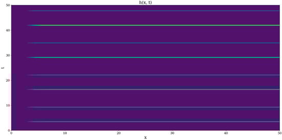
Figure 1. Example plot of h(x,t); ω constant.

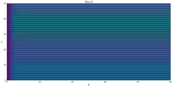
Figure 2. Example plot of h(x,t); ω constant odd integer.

These plots show that oscillatory components can exist in the complex systems at all scales; interestingly, $\mathrm{h}$ manifests ordered predictable peaks whose intensity tends to slightly increase in time, but only if $\mathsf{\omega }$ is an odd integer (Figure 1 and Figure 2). Otherwise, other plotting instances show relatively disordered and unpredictable distributions of these peaks. It can be interpreted that an undulatory-corpuscular duality can be observed through this behavior, with odd integer $\mathsf{\omega }$ representing the damping oscillatory behavior and all other cases producing corpuscular behavior (Figure 1 and Figure 2). We note that in the behavior manifested in Figure 1 and Figure 2, discontinuities are induced by the interactions between the complex system entities (more precisely, through the interaction strength between the complex system entities).

Now, for in-phase coherences of the complex system entities, for example: ${\mathrm{e}}^{\mathrm{is}}=1$ which implies $\mathrm{s}=2\mathsf{\pi }\mathrm{n}, \mathrm{n}\in \mathbb{Z}$, $\mathsf{\psi }$ becomes:

$$\mathsf{\psi }=\sqrt{\rho }\frac{\mathrm{h}\overline{\mathrm{h}}-1}{\mathrm{h}\overline{\mathrm{h}}+1}$$

(39)

The produced plots show instances of the states function manifesting in a sporadic and periodic manner, with varying spatial dimensions (Figure 3 and Figure 4). Given the fact that, at this point, the only control parameter of $\mathsf{\psi }$ is $\mathsf{\omega }$, no other constant will affect the behavior of the function of the state; furthermore, even the choice of this parameter does not seem to fundamentally affect the dynamical regime of $\mathsf{\psi }$, which manifests multifractal states of varying length fluctuating in time (Figure 3 and Figure 4). These fluctuations show the spontaneous and periodical occurrence of multifractal structures in the given multifractal flow. Worth noting, however, is the fact that the areas of the plot that manifest no color at all are in fact not areas where the states function is zero, but are areas where the $\mathsf{\psi }$ calculation yields cases of non-determination, and thus these are regions where it is absolutely impossible for states to exist. Moreover, a completely different fine structure exists at small scales compared to large scales, wherein vanishing states are manifested, and the appearance of these intense negative fluctuations manifests absolutely no periodicity (Figure 3 and Figure 4).

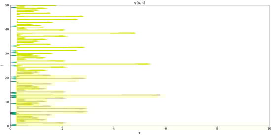
Figure 3. Example plot of ψ(x,t); ω constant.

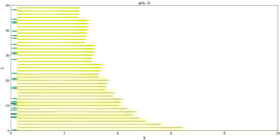
Figure 4. Example plot of ψ(x,t); ω constant odd integer.

In performing the first step of our analysis, the inhomogeneity map of the multifractal non-differentiable mass conduction needs to be performed. By definition, the total inhomogeneity of any parameter in a given volume V of atmospheric fluid is [18]:

$$\mathrm{G}=\frac{1}{2}{\displaystyle \int }⟨{{\mathsf{\vartheta }}^{\prime }}^2⟩\mathrm{dV}$$

(40)

Given a non-strict dependency on spatial conditions, and the non-dimensionality entailed throughout much of the previous analysis, it will suffice to perform $⟨{\left|\overline{{\mathsf{\sigma }}_{\mathrm{F}}}\right|}^{{}^{\prime }2}⟩$. Through a Reynolds decomposition, the following is obtained [18,19]:

$$⟨{\left|\overline{{\mathsf{\sigma }}_{\mathrm{F}}}\right|}^{{}^{\prime }2}⟩=⟨{\left(\left|\overline{{\mathsf{\sigma }}_{\mathrm{F}}}\right|-⟨\left|\overline{{\mathsf{\sigma }}_{\mathrm{F}}}\right|⟩\right)}^2⟩$$

(41)

This can then be iterated across the fractal dimension in a bifurcation map, where we have noted $\mathrm{x}\equiv \mathsf{\theta },\mathrm{t}\equiv \mathsf{\eta }$ (Figure 5, Figure 6, Figure 7, Figure 8, Figure 9, Figure 10, Figure 11 and Figure 12).

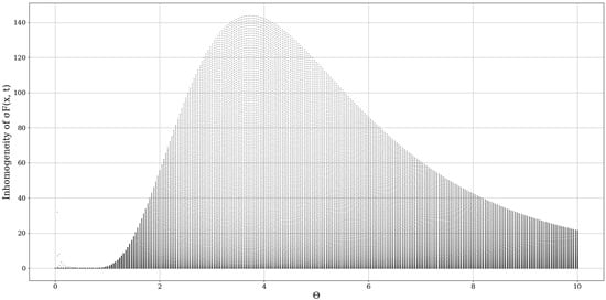
Figure 5. $⟨{\left|\overline{{\mathsf{\sigma }}_{\mathrm{F}}}\right|}^{{}^{\prime }2}⟩$ example plot with θ as control parameter; ξ = 0.5; μ = 1.

Figure 6. $⟨{\left|\overline{{\mathsf{\sigma }}_{\mathrm{F}}}\right|}^{{}^{\prime }2}⟩$ example plot with θ as control parameter; ξ = 3; μ = 1.

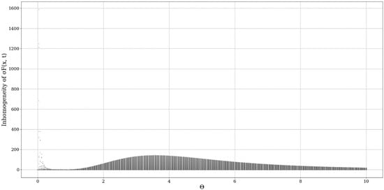
Figure 7. $⟨{\left|\overline{{\mathsf{\sigma }}_{\mathrm{F}}}\right|}^{{}^{\prime }2}⟩$ example plot with θ as control parameter; ξ = 6; μ = 1.

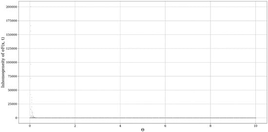
Figure 8. $⟨{\left|\overline{{\mathsf{\sigma }}_{\mathrm{F}}}\right|}^{{}^{\prime }2}⟩$ example plot with θ as control parameter; ξ = 9; μ = 1.

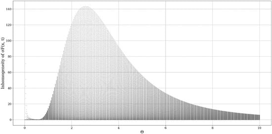
Figure 9. $⟨{\left|\overline{{\mathsf{\sigma }}_{\mathrm{F}}}\right|}^{{}^{\prime }2}⟩$ example plot with θ as control parameter; ξ = 3; μ = 0.5.

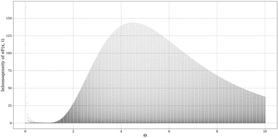
Figure 10. $⟨{\left|\overline{{\mathsf{\sigma }}_{\mathrm{F}}}\right|}^{{}^{\prime }2}⟩$ example plot with θ as control parameter; ξ = 3; μ = 3.

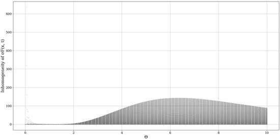
Figure 11. $⟨{\left|\overline{{\mathsf{\sigma }}_{\mathrm{F}}}\right|}^{{}^{\prime }2}⟩$ example plot with θ as control parameter; ξ = 3; μ = 6.

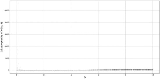
Figure 12. $⟨{\left|\overline{{\mathsf{\sigma }}_{\mathrm{F}}}\right|}^{{}^{\prime }2}⟩$ example plot with θ as control parameter; ξ = 3; μ = 9.

It seems that $\mathsf{\xi }$ plays the role of a spatial limiting factor, dictating the conduction band intensity, and it is to be expected that a constant inversely proportional to the initial value of the differentiable velocity field would play an important role here (Figure 5, Figure 6, Figure 7 and Figure 8).

Modifying the multifractal-nonmultifractal scale transition constant μ appears to have relatively similar effects to the inhomogeneity map; however, it affects not only the intensity but also the relative shape of the conduction bands (Figure 9, Figure 10, Figure 11 and Figure 12). All cases exhibit what are practically two peak-like structures; one of them found at low values of $\mathsf{\theta }$, which shows a very high value variability and unpredictability. Otherwise, the exact value of $\mathsf{\tau }$ does not seem to affect the dynamic regime of the modeled behavior.

4. Results

In any case, it seems that the inhomogeneity analysis points to very dynamic behavior, however, a constant aspect is that indifferent to the values being chosen, one or more inhomogeneity peaks always appear at certain values of $\mathsf{\theta }$, and thus, at certain fractal dimensions. While this peak can apparently be shifted or modified, it almost always exists, pointing to the existence of certain dimensions, at certain atmospheric parameters, that entail high unpredictability and values of conduction. This then means that, if certain conditions are fulfilled, inversions of fractal dimensions might lead to unpredictability and high values of multifractal non-differentiable mass conduction. The exact values of the fractal dimension would not be important here, however, jumps or inversions of the atmospheric fractal dimension would imply special behaviors of atmospheric conduction, which would then either create stability or instability as a function of the fractal dimension.

For parallels to be drawn between theory and experimental data, experimental ceilometer data must be produced. This data shall be used to calculate the initial and final turbulent scales in order for the atmospheric fractal dimension profile to be obtained, and for this, the structure coefficient of the refraction index profile ${\mathrm{C}}_{\mathrm{N}}^{2 }\left(\mathrm{L}\right)$ is obtained by [18,20]:

$${ \mathsf{\sigma }}_{\mathrm{I}}^2\left(\mathrm{L}\right)=1.23{ \mathrm{C}}_{\mathrm{N}}^{2 }\left(\mathrm{L}\right){\mathrm{k}}^{\frac{7}{6}}{\mathrm{L}}^{\frac{11}{6}}$$

(42)

in which we have named ${ \mathsf{\sigma }}_{\mathrm{I}}^2$ the scintillation of a source of light observed from a distance represented by the optical path $\mathrm{L}$. In this case, the source of light itself is the point in the optical path at which ceilometer light is being backscattered. Meanwhile, $\mathrm{I}$ refers to the intensity of the backscattered range-corrected lidar signal at a particular point in the optical path, or the $\mathrm{RCS}$ (range-corrected signal) intensity, which will be used to find ${ \mathsf{\sigma }}_{\mathrm{I}}^2$ [13,14,18,20]. In past studies, it has been deemed and proved sufficient to employ three $\mathrm{RCS}$ profiles in the averaging process. After the ${\mathrm{C}}_{\mathrm{N}}^{2 }$ profile has been determined, it is now possible to calculate the length scales with various approximations. The inner scale profile is linked to scintillation:

$${\mathsf{\sigma }}_{\mathrm{I}}^2\left(\mathrm{L}\right)\cong 0.615{ \mathrm{C}}_{\mathrm{N}}^{2 }\left(\mathrm{L}\right){\mathrm{L}}^3{\mathrm{l}}_{\mathrm{d}}{\left(\mathrm{L}\right)}^{\frac{-7}{3}}$$

(43)

and the outer scale can be connected to the ${ \mathrm{C}}_{\mathrm{N}}^{2 }$ profile:

$${\mathrm{C}}_{\mathrm{N}}^2\left(\mathrm{z}\right)={ \mathrm{L}}_0{\left(\mathrm{z}\right)}^{\frac{4}{3}}{\left(\nabla ⟨\mathrm{n}\left(\mathrm{z}\right)⟩\right)}^2$$

(44)

For atmospheric turbulent eddies in the inertial subrange, the following approximation is possible:

$$\mathrm{n}\left(\mathrm{z}\right)\cong {\mathrm{n}}_0-\sqrt{{\mathrm{C}}_{\mathrm{N}}^2\left(\mathrm{z}\right){\mathrm{z}}^{\frac{2}{3}}}$$

(45)

which can then be used to extract the outer scale profile. This method is well-referenced in our studies and has been already used successfully multiple times.

When introducing the ceilometer data plots, technical details must be presented; the platform used to produce this data is described in the following segment. The platform utilized in this study is a CHM15k ceilometer operating at a $1064 \mathrm{nm}$ wavelength, positioned in Galați, Romania, at the UGAL–REXDAN facility found at the coordinates $45.435125\mathrm{N}$, $28.036792\mathrm{E}$, $65 \mathrm{m}$ ASL, which is a part of the “Dunărea de Jos” University of Galați. The instrument itself has been chosen so as to conform to the standards imposed by the ACTRIS community. From a computational perspective, the necessary calculations are performed through code written and operated in Python 3.6.

These sets of ceilometer data were profiled on the 22nd and 23nd of December 2021, starting right before noon. Many typical features of the atmosphere, including aerosol plumes, clouds and the PBL, along with its variation, can be observed in the $\mathrm{RCS}$ data (Figure 13, Figure 14, Figure 15 and Figure 16). Despite the presence of many cloud-type structures, the lower part of the time series is generally unaffected and can be analyzed. The start of the time series shows a convective mixed layer typical of noon conditions, and in the latter stages of the time series, the stratified structure of the stable boundary layer (SBL) and the residual layer (RL)—the gap between them, which we shall name “the double layer”—is delineated by the region of low $\mathrm{RCS}$ intensity [21,22] (Figure 13, Figure 14, Figure 15 and Figure 16).

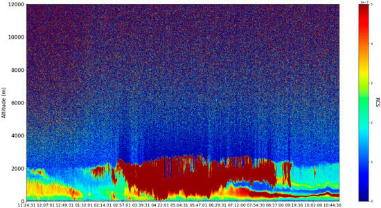
Figure 13. RCS time series, λ = 1064 nm, Galați, Romania, 23 December 2021.

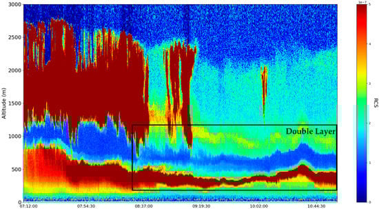
Figure 14. Zoomed-in (region of interest) RCS time series, λ = 1064 nm, Galați, Romania, 23 December 2021.

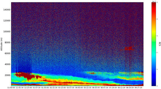
Figure 15. RCS. time series, λ = 1064 nm, Galați, Romania, 22 December 2021.

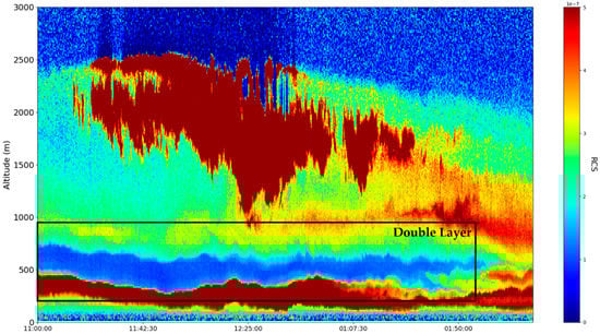
Figure 16. Zoomed-in (region of interest) RCS time series, λ = 1064 nm, Galați, Romania, 22 December 2021.

The ${\mathrm{C}}_{\mathrm{N}}^2$ profile can be commonly used as an indicator of atmospheric turbulence strength; it can be also used to more accurately quantify the PBL altitude, and to identify regions of atmospheric calm or extreme turbulence (Figure 17, Figure 18, Figure 19 and Figure 20) [13,14]. The region of delineation between the SBL and the RL can also be seen, and while the RCS indicated a region of lower intensity and thus of a lower concentration of atmospheric components, ${\mathrm{C}}_{\mathrm{N}}^2$ time series shows higher activities, especially at the limits of the SBL and RL itself (Figure 17, Figure 18, Figure 19 and Figure 20). Higher ${\mathrm{C}}_{\mathrm{N}}^2$ implies higher degrees of turbulence, which implies greater mixing. However, ${\mathrm{C}}_{\mathrm{N}}^2$ reduces abruptly beyond the boundary between the SBL and the RL, which indicates that this increased mixing, which is limited only to the interior of the apparent boundary layer, implies that the atmospheric matter found in the boundary layer is being shifted upwards and downwards into the SBL and the RL. This, then explains why fewer backscatterings of atmospheric matter can be found, and why the RCS intensity is lower in that region (Figure 17, Figure 18, Figure 19 and Figure 20).

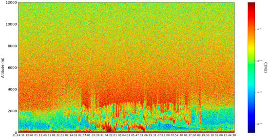
Figure 17. ${\mathrm{C}}_{\mathrm{N}}^2$ time series, λ = 1064 nm, Galați, Romania, 23 December 2021.

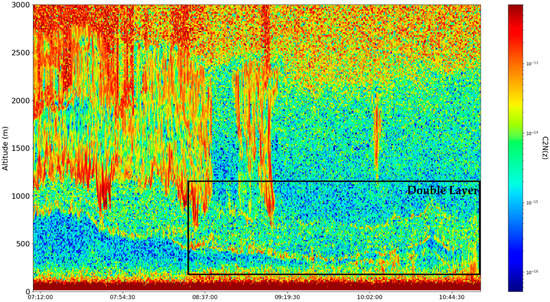
Figure 18. Zoomed-in (region of interest) ${\mathrm{C}}_{\mathrm{N}}^2$ time series, λ = 1064 nm, Galați, Romania, 23 December 2021.

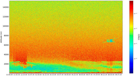
Figure 19. ${\mathrm{C}}_{\mathrm{N}}^2$ time series, λ = 1064 nm, Galați, Romania, 22 December 2021.

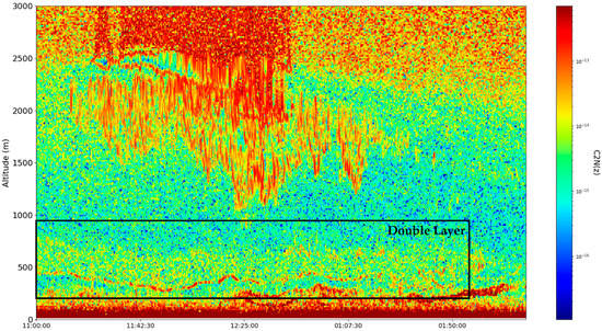
Figure 20. Zoomed-in (region of interest) ${\mathrm{C}}_{\mathrm{N}}^2$ time series, λ = 1064 nm, Galați, Romania, 22 December 2021.

Since the minimal fractal dimension of atmospheric turbulent vortices, in general, is logically $2$ since vortices are by definition at least two-dimensional, and the maximal fractal dimension of atmospheric turbulent vortices is 3, it can be entirely expected for the average of these vortices, as plotted in Figure 21, Figure 22, Figure 23 and Figure 24, to be quite close to $3$ because such dimensions rapidly increase asymptotically towards 3 in the turbulent cascade [14]. In any case, lower fractal dimensions, especially sudden spatial decreases of fractal dimensions, point towards ordering and autostructuring—this is partially confirmed by the fact that the atmospheric cloud structure present in the time series manifests sudden and markedly-lower transitions of fractal dimensions, as expected for relatively orderly atmospheric structures, such as clouds (Figure 21, Figure 22, Figure 23 and Figure 24). This autostructuring then also entails the existence of the boundaries between the SBL and the RL, because, for the boundary to exist, it must be stable—however, this seems to be a type of “dynamic stability”, one marked by higher turbulence and mass transfer from the boundary area to the SBL and the RL. Furthermore, we have previously determined that inversions of fractal dimensions might lead to unpredictability and high values of multifractal non-differentiable mass conduction, and these inversions are exactly what we see at the boundary edges between the SBL and the RL, thus confirming the conduction theory presented in this study.

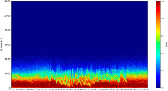
Figure 21. D_f time series, λ = 1064 nm, Galați, Romania, 23 December 2021.

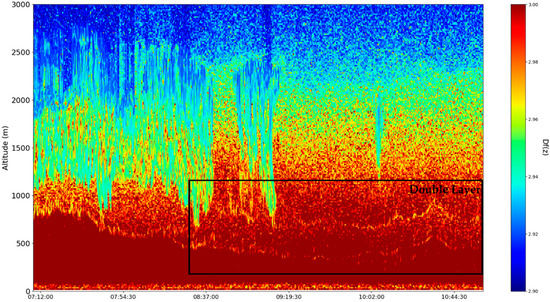
Figure 22. Zoomed-in (region of interest) D_f time series, λ = 1064 nm, Galați, Romania, 23 December 2021.

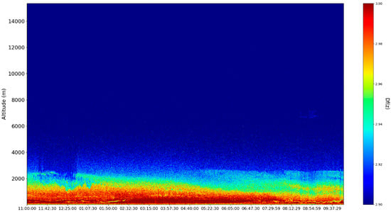
Figure 23. D_f time series, λ = 1064 nm, Galați, Romania, 22 December 2021.

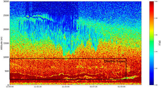
Figure 24. Zoomed-in (region of interest) D_f time series, λ = 1064 nm, Galați, Romania, 22 December 2021.

5. Conclusions

Applying the multifractal theory of motion to atmospheric entities through a hydrodynamic multifractal scenario, a multifractal conservation law that leads to differentiable and non-differentiable velocity fields is found; this then implies, through various nondimensionalizations, the existence of a specific multifractal force field that drives non-differentiable interactions between the atmospheric multifractal entities. Supposing then, that there exists a mass current density-type relation regarding these entities, then multifractal atmospheric mass conduction is found at differentiable, non-differentiable and global resolutions. In order for the exact form of this conduction to be found, a Lobachevsky plane metric is employed to find a component of the state function described by the multifractal conservation law. The inhomogeneity of the non-differentiable conduction is then analyzed regarding the fractal dimension variation, and it is found that there exist certain fractal dimensions where the non-differentiable conduction can present large fluctuations and values.

This then implies that, at fractal dimension inversions, intense non-differentiable conduction phenomena can occur, leading to vertical mass conduction and the formation of certain stable atmospheric features. Finally, ceilometer data is introduced, and this data is used in order to construct various time series profiles, including time series of the atmospheric fractal dimension. Fractal dimension inversions are observed in connection to the SBL and RL boundaries, which then validates that such inversions can lead to phenomena of mass conduction and atmospheric structure stability. There are possible limitations to the employed method, mainly regarding rapid aerosol intrusions—generally speaking, the associated multifractal and ceilometer theory works best only in relatively calm conditions, without the appearance of unexpected cloud or aerosol concentrations. Further studies could include further theoretical and practical validation that employs climatic models, such as ALARO or WRF, and such studies could also utilize larger batches of ceilometer data.

References

- Bar-Yam, Y.; McKay, S.R.; Christian, W. Dynamics of Complex Systems (Studies in Nonlinearity). Comput. Phys. 1998, 12, 335–336. [Google Scholar] [CrossRef] [Green Version]
- Mitchell, M. Complexity: A Guided Tour; Oxford University Press: Oxford, UK, 2009. [Google Scholar]
- Badii, R.; Politi, A. Complexity: Hierarchical Structures and Scaling in Physics; Cambridge University Press: Cambridge, UK, 1999; p. 6. [Google Scholar]
- Flake, G.W. The Computational Beauty of Nature: Computer Explorations of Fractals, Chaos, Complex Systems, and Adaptation; MIT Press: Cambridge, MA, USA, 1998. [Google Scholar]
- Țîmpu, S.; Sfîcă, L.; Dobri, R.V.; Cazacu, M.M.; Nita, A.I.; Birsan, M.V. Tropospheric Dust and Associated Atmospheric Circulations over the Mediterranean Region with Focus on Romania’s Territory. Atmosphere 2020, 11, 349. [Google Scholar] [CrossRef] [Green Version]
- Baleanu, D.; Diethelm, K.; Scalas, E.; Trujillo, J.J. Fractional Calculus: Models and Numerical Methods; World Scientific: Singapore, 2012; Volume 3. [Google Scholar]
- Ortigueira, M.D. Fractional Calculus for Scientists and Engineers; Springer Science & Business Media: Berlin, Germany, 2011; Volume 84. [Google Scholar]
- Nottale, L. Scale Relativity and Fractal Space-Time: A New Approach to Unifying Relativity and Quantum Mechanics; Imperial College Press: London, UK, 2011. [Google Scholar]
- Merches, I.; Agop, M. Differentiability and Fractality in Dynamics of Physical Systems; World Scientific: Singapore, 2015. [Google Scholar]
- Mandelbrot, B.B. The Fractal Geometry of Nature; WH Freeman: San Francisco, CA, USA, 1982. [Google Scholar]
- Jackson, E.A. Perspectives of Nonlinear Dynamics; CUP Archive: Cambridge, UK, 1989; Volume 1. [Google Scholar]
- Cristescu, C.P. Nonlinear Dynamics and Chaos. Theoretical Fundaments and Application; Romanian Academy Publishing House: Bucharest, Romania, 1987. [Google Scholar]
- Roşu, I.A.; Cazacu, M.M.; Ghenadi, A.S.; Bibire, L.; Agop, M. On a multifractal approach of turbulent atmosphere dynamics. Front. Earth Sci. 2020, 8, 216. [Google Scholar] [CrossRef]
- Roșu, I.A.; Cazacu, M.M.; Agop, M. Multifractal Model of Atmospheric Turbulence Applied to Elastic Lidar Data. Atmosphere 2021, 12, 226. [Google Scholar] [CrossRef]
- Mazilu, N.; Agop, M. Skyrmions: A Great Finishing Touch to Classical Newtonian Philosophy; World Philosophy Series; Nova: New York, NY, USA, 2012. [Google Scholar]
- Mazilu, N.; Agop, M.; Merches, I. Scale Transitions as Foundations of Physics; World Scientific: Singapore, 2021. [Google Scholar]
- Xin, Y. Geometry of Harmonic Maps (Vol. 21); Springer Science & Business Media: Heidelberg, Germany, 1996. [Google Scholar]
- Tatarski, V.I. Wave Propagation in a Turbulent Medium; Courier Dover Publications: New York, NY, USA, 2016. [Google Scholar]
- Alfonsi, G. Reynolds-averaged Navier–Stokes equations for turbulence modeling. Appl. Mech. Rev. 2009, 62, 040802. [Google Scholar] [CrossRef]
- Rosu, I.A.; Cazacu, M.M.; Prelipceanu, O.S.; Agop, M. A Turbulence-Oriented Approach to Retrieve Various Atmospheric Parameters Using Advanced Lidar Data Processing Techniques. Atmosphere 2019, 10, 38. [Google Scholar] [CrossRef] [Green Version]
- Busch, N.E. The surface boundary layer. Bound. Layer Meteorol. 1973, 4, 213–240. [Google Scholar] [CrossRef]
- Haeffelin, M.; Angelini, F.; Morille, Y.; Martucci, G.; Frey, S.; Gobbi, G.P.; Lolli, S.; O’Dowd, C.D.; Sauvage, L.; Xueref-Rémy, I.; et al. Evaluation of mixing-height retrievals from automatic profiling lidars and ceilometers in view of future integrated networks in Europe. Bound. Layer Meteorol. 2012, 143, 49–75. [Google Scholar] [CrossRef]
Publisher’s Note: MDPI stays neutral with regard to jurisdictional claims in published maps and institutional affiliations. |
© 2022 by the authors. Licensee MDPI, Basel, Switzerland. This article is an open access article distributed under the terms and conditions of the Creative Commons Attribution (CC BY) license (https://creativecommons.org/licenses/by/4.0/).