Lyapunov Direct Method for Nonlinear Hadamard-Type Fractional Order Systems

Abstract

In this paper, a rigorous Lyapunov direct method (LDM) is proposed to analyze the stability of fractional non-linear systems involving Hadamard or Caputo–Hadamard derivatives. Based on the characteristics of Hadamard-type calculus, several new inequalities are derived for different definitions. By means of the developed inequalities and modified Laplace transform, the sufficient conditions can be derived to guarantee the Hadamard–Mittag–Leffler (HML) stability of the systems. Lastly, two illustrative examples are given to show the effectiveness of our proposed results.

1. Introduction

Over the last two decades, fractional calculus has been shown to be a powerful tool for modeling some non-classical phenomena in nature and society [1,2]. Fractional differential equations can describe materials and processes with memory, inheritance, and non-locality more compatible than the corresponding integer order models [3], such as viscoelastic systems, signal processing, electrochemistry, biology, biophysics, and so on [4,5,6,7,8,9]. In order to characterize the differences between these features, many different types fractional calculus have been proposed, such as Riemann–Liouville, Caputo, and Hadamard [10,11].

A large number of papers and books have studied the typical fractional derivatives (Riemann–Liouville and Caputo) [12,13,14,15,16,17,18], but Hadamard and Caputo–Hadamard derivatives are also worth further study. There are many differences between the Hadamard calculus and typical fractional ones: the kernel function of the former is logarithmic form ${(log\frac{t}{t_0})}^{\alpha -1}$, while that of the latter is power form ${(t-s)}^{\alpha -1}$; the former can be viewed as a generalization of the form ${\left(t\frac{\mathrm{d}}{\mathrm{d}t}\right)}^n$, and the latter can be thought of as a extension of classical derivatives ${\left(\frac{\mathrm{d}}{\mathrm{d}t}\right)}^n$. The solutions of Hadamard-type differential equations can own logarithmic decay ${(log\frac{t}{t_0})}^{-\alpha }$, but typical fractional differential equations have the power-law decay $t^{-\alpha }$ [19]. In addition, the Hadamard-type calculus are widely applied to practical problems in mechanics and engineering, such as crack problems, fracture analysis [20], and igneous rock [21,22].

There is no doubt that stability analysis is a core problem for fractional systems. Many papers have focused on the stability of Riemann–Liouville and Caputo fractional systems, such as Caputo linear systems [23], Caputo non-linear systems [24,25,26], Caputo time-delay systems [27], Riemann–Liouville non-linear systems [28], Riemann–Liouville time-varying delays systems [29], and so on. However, there are few topics on the stability of Hadamard and Caputo–Hadamard fractional systems. It should be note that Li et al. [19] investigated the logarithmic decay of fractional Hadamard and Caputo–Hadamard systems. Ma et al. [30] discussed the finite-time stability of Hadamard-type systems.

It is well known that the LDM provides a handy tool for the stability analysis of fractional non-linear systems. There are two main aspects to illustrate its importance: on the one hand, this technique allows to formalize practical goals; on the other hand, LDM obtain the stability of a wide class of fractional systems without explicitly solving it. The LDM refers to look for a Lyapunov function for a non-linear differential equation. The LDM is only a sufficient condition for proving the stability, which means that the non-linear system may be stable, even if the Lyapunov function is not found. However, it is not easy to construct an appropriate Lyapunov function, due to there being few practical algebraic criteria for fractional systems.

Inspired by the above discussion, this paper studies the LDM of Hadamard-type fractional non-linear systems, aiming to give some simple criteria of stability. Firstly, several new Hadamard-type fractional inequalities are given, which extend the applications of Hadamard calculus. Then, the asymptotic stability of Hadamard and Caputo–Hadamard non-autonomous systems are obtained by LDM. Finally, two examples are given to illustrate the efficiency of the developed theory by the predictor–corrector algorithm.

The layout of the current paper is structured as follows. Section 2 introduces some necessary definitions and lemmas. Section 3 develops several inequalities. Section 4 proves Hadamard-type Lyapunov stability theorems. Section 5 verifies the proposed methods with two examples. Section 6 summarizes the results.

2. Preliminaries

In this part, some necessary definitions and lemmas about stability analysis of Hadamard-type systems are given.

Definition 1

([31]). The Hadamard integral of function $f\left(t\right)$ is defined by

$$\begin{array}{c}\hfill {}_H{\mathrm{D}}_{t_0,t}^{-\alpha }f\left(t\right)=\frac{1}{\Gamma \left(\alpha \right)}{\int }_{t_0}^t{\left(log\frac{t}{s}\right)}^{\alpha -1}f\left(s\right)\frac{ds}{s},\end{array}$$

where $0<t_0<t$ and $\alpha >0$.

Definition 2

([31]). The Hadamard derivative of function $f\left(t\right):(t_0,+\infty )\to \mathbb{R}$ is defined by

$$\begin{array}{c}\hfill {}_H{\mathrm{D}}_{t_0,t}^{\alpha }f\left(t\right)=\frac{1}{\Gamma (n-\alpha )}{\delta }^n{\int }_{t_0}^t{\left(log\frac{t}{s}\right)}^{n-\alpha -1}f\left(s\right)\frac{ds}{s},\end{array}$$

where $t_0>0,\delta =t\frac{d}{dt}$, and $n-1<\alpha <n\in {\mathbb{Z}}^{+}$.

Definition 3

([32]). The Caputo–Hadamard derivative of function $f\left(t\right):(t_0,+\infty )\to \mathbb{R}$ is defined by

$$\begin{array}{c}\hfill {}_{CH}{\mathrm{D}}_{t_0,t}^{\alpha }f\left(t\right)=\frac{1}{\Gamma (n-\alpha )}{\int }_{t_0}^t{\left(log\frac{t}{s}\right)}^{n-\alpha -1}{\left(s\frac{d}{ds}\right)}^{n}f\left(s\right)\frac{ds}{s},\end{array}$$

where $t_0>0$, and $n-1<\alpha <n\in {\mathbb{Z}}^{+}$.

Obviously ${}_{CH}{\mathrm{D}}_{t_0,t}^{\alpha }C=0,\forall C\in \mathbb{R}$.

Lemma 1

([1,32,33]). Let $\alpha ,\beta \in (0,1)$, and $t_0>0$. Then, the following relationships hold:

$$\begin{array}{}\mathrm{(1)}& \left(i\right)\hfill & {}_{CH}{\mathrm{D}}_{t_0,t}^{\alpha }f\left(t\right)={}_H{\mathrm{D}}_{t_0,t}^{\alpha }f\left(t\right)-\frac{f\left(t_0\right)}{\Gamma (1-\alpha )}{(log\frac{t}{t_0})}^{-\alpha };\hfill \mathrm{(2)}& \left(ii\right)\hfill & {}_H{\mathrm{D}}_{t_0,t}^{-\alpha }{(}_H{\mathrm{D}}_{t_0,t}^{-\beta }f\left(t\right))={}_H{\mathrm{D}}_{t_0,t}^{-(\alpha +\beta )}f\left(t\right);\hfill \mathrm{(3)}& \left(iii\right)\hfill & {}_H{\mathrm{D}}_{t_0,t}^{-\alpha }{(}_{CH}{\mathrm{D}}_{t_0,t}^{\alpha }f\left(t\right))=f\left(t\right)-f\left(t_0\right).\hfill \end{array}$$

Lemma 2

([34]). Let ${\pounds }_m$ be the modified Laplace transform. Then, the following relationships hold:

$$\begin{array}{}\mathrm{(4)}& \left(i\right)\hfill & {\pounds }_m{\{}_H{\mathrm{D}}_{t_0^{+}}^{-\alpha }f\left(t\right)\}=s^{-\alpha }{\pounds }_m\left\{f\left(t\right)\right\};\hfill \mathrm{(5)}& \left(ii\right)\hfill & {\pounds }_m{\{}_H{\mathrm{D}}_{t_0,t}^{\alpha }f\left(t\right)\}=s^{\alpha }{\pounds }_m\left\{f\left(t\right)\right\}-\sum _{k=0}^{n-1}{s}^{n-k-1}\left[{\delta }^k{}_H{D}_{t_0,t}^{-(n-\alpha )}f\left(t\right)\right]{|}_{t=t_0};\hfill \mathrm{(6)}& \left(iii\right)\hfill & {\pounds }_m{\{}_{CH}{\mathrm{D}}_{t_0,t}^{\alpha }f\left(t\right)\}=s^{\alpha }{\pounds }_m\left\{f\left(t\right)\right\}-\sum _{k=0}^{n-1}{s}^{\alpha -k-1}{\delta }^{k}f\left(t_0\right),\hfill \end{array}$$

where $n-1<\alpha <n\in {\mathbb{Z}}^{+}$ and $t_0>0$.

Lemma 3

([34]). Let $E_{\alpha ,\beta }\left(z\right)={\sum }_{k=0}^{\infty }\frac{z^k}{\Gamma (\alpha k+\beta )}$ be the Mittag–Leffler function. Then, there holds

$$\begin{array}{c}\hfill {\pounds }_m\left\{{\left(log\frac{t}{t_0}\right)}^{\alpha k+\beta -1}{E}_{\alpha ,\beta }^{\left(k\right)}\left(\pm \eta {\left(log\frac{t}{t_0}\right)}^{\alpha }\right)\right\}=\frac{k!s^{\alpha -\beta }}{{(s^{\alpha }\mp \eta )}^{k+1}},\end{array}$$

where ${Re\left(s\right)>\left|\eta \right|}^{\frac{1}{\alpha }},\alpha >0,\beta >0,z\in \mathbb{C}$, and $E_{\alpha ,\beta }^{\left(k\right)}\left(y\right)=:\frac{d^k}{d{y}^k}{E}_{\alpha ,\beta }\left(y\right)$.

Lemma 4

([34]). Assume ${\pounds }_m\left\{\phi \left(t\right)\right\}=\tilde{\phi }\left(s\right)$ and ${\pounds }_m\left\{\psi \left(t\right)\right\}=\tilde{\psi }\left(s\right)$, then

$$\begin{array}{c}\hfill {\pounds }_m\{\phi \left(t\right)\ast \psi \left(t\right)\}={\pounds }_m\left\{\phi \left(t\right)\right\}{\pounds }_m\left\{\psi \left(t\right)\right\}=\tilde{\phi }\left(s\right)\tilde{\psi }\left(s\right),\end{array}$$

and

$$\begin{array}{c}\hfill {\pounds }_m^{-1}\left\{\tilde{\phi }\left(s\right)\tilde{\psi }\left(s\right)\right\}=\phi \left(t\right)\ast \psi \left(t\right),\end{array}$$

where ${\pounds }_m^{-1}$ is the inverse modified Laplace transform, and the convolution ∗ is defined by

$$\begin{array}{c}\hfill \phi \left(t\right)\ast \psi \left(t\right)={\int }_{t_0}^t\phi \left(t_0\frac{t}{\tau }\right)\psi \left(\tau \right)\frac{d\tau }{\tau }.\end{array}$$

(7)

Lemma 5

([33]). Let $f(t,\phi (t\left)\right)$ be locally Lipschitz continuous in $\phi \left(t\right)$ for any $t>t_0$. Assume $\phi \left(t\right)$ and $\psi \left(t\right)$ are continuous functions satisfying Caputo–Hadamard fractional equations ${}_{CH}{\mathrm{D}}_{t_0,t}^{\alpha }\phi \left(t\right)=f(t,\phi \left(t\right))$ and ${}_{CH}{\mathrm{D}}_{t_0,t}^{\alpha }\psi \left(t\right)\le f(t,\psi \left(t\right))$, $\alpha \in (0,1)$, respectively. If $\psi \left(t_0\right)\le \phi \left(t_0\right)$, then one has $\psi \left(t\right)\le \phi \left(t\right)$.

Lemma 6

([35]). Let $\lambda \left(A\right)$ be the eigenvalues of matrix $A\in {\mathbb{C}}^{n\times n}$. If $0<\alpha <2,\beta \in \mathbb{R},\frac{\pi \alpha }{2}<u<min\{\pi ,\pi \alpha \},u\le arg\left(\lambda \left(A\right)\right)\le \pi$ and $\gamma >0$, then

$$\begin{array}{c}\hfill \parallel E_{\alpha ,\beta }\left(A\right)\parallel \le \frac{\gamma }{1+\parallel A\parallel },\end{array}$$

where $\parallel ·\parallel$ is the $l_2$-norm.

3. Hadamard-Type Fractional Inequalities

In this part, some Hadamard-type fractional inequalities are given, which are very important in the stability analysis.

Theorem 1.

For the continuous function $f(t,\phi (t\left)\right)$, one gets

$$\begin{array}{c}\hfill {\parallel }_H{\mathrm{D}}_{t_0,t}^{-\alpha }f(t,\phi \left(t\right)\parallel \le {}_H{\mathrm{D}}_{t_0,t}^{-\alpha }\parallel f(t,\phi \left(t\right)\parallel ,\end{array}$$

where $\alpha >0$ and $t>t_0>0$.

Proof. 

From the Definition 1, one has

$$\begin{array}{cc}\hfill \parallel {}_H{\mathrm{D}}_{t_0,t}^{-\alpha }f(t,\phi \left(t\right))\parallel & =\parallel \frac{1}{\Gamma \left(\alpha \right)}{\int }_{t_0}^t{\left(log\frac{t}{s}\right)}^{\alpha -1}f(s,\phi \left(s\right))\frac{ds}{s}\parallel \hfill \\ \hfill & \le \frac{1}{\Gamma \left(\alpha \right)}{\int }_{t_0}^t{\left(log\frac{t}{s}\right)}^{\alpha -1}\parallel f(s,\phi \left(s\right))\parallel \frac{ds}{s}\hfill \\ \hfill & ={}_H{\mathrm{D}}_{t_0,t}^{-\alpha }\parallel f(t,\phi \left(t\right))\parallel .\hfill \end{array}$$

□

Theorem 2.

Let $x\left(t\right)\in \mathbb{R},\alpha \in (0,1),X\left(t\right)\in {\mathbb{R}}^n$, and $M\in {\mathbb{R}}^{n\times n}$ be a positive definite matrix. Then, the following inequalities hold:

$$\begin{array}{}\mathrm{(8)}& \left(i\right)\hfill & {}_{CH}{\mathrm{D}}_{t_0,t}^{\alpha }{x}^{2m}\left(t\right)\le 2x^m\left(t\right){}_{CH}{\mathrm{D}}_{t_0,t}^{\alpha }{x}^m\left(t\right);\hfill \mathrm{(9)}& \left(ii\right)\hfill & {}_{CH}{\mathrm{D}}_{t_0,t}^{\alpha }{x}^{\frac{2m}{n}}\left(t\right)\le \frac{2m}{2m-n}x\left(t\right){}_{CH}{\mathrm{D}}_{t_0,t}^{\alpha }{x}^{\frac{2m}{n}-1}\left(t\right);\hfill \mathrm{(10)}& \left(iii\right)\hfill & {}_{CH}{\mathrm{D}}_{t_0,t}^{\alpha }{x}^{\frac{2m}{n}}\left(t\right)\le \frac{2m}{n}{x}^{\frac{2m}{n}-1}\left(t\right){}_{CH}{\mathrm{D}}_{t_0,t}^{\alpha }x\left(t\right);\hfill \mathrm{(11)}& \left(iv\right)\hfill & {}_{CH}{\mathrm{D}}_{t_0,t}^{\alpha }{x}^{2^m}\left(t\right)\le 2^m{x}^{2^m-1}\left(t\right){}_{CH}{\mathrm{D}}_{t_0,t}^{\alpha }x\left(t\right);\hfill \mathrm{(12)}& \left(v\right)\hfill & {}_{CH}{\mathrm{D}}_{t_0,t}^{\alpha }\left(X^{\top }\left(t\right)MX\left(t\right)\right)\le 2X^{\top }\left(t\right)M{}_{CH}{\mathrm{D}}_{t_0,t}^{\alpha }X\left(t\right),\hfill \end{array}$$

where $t>t_0,m\in {\mathbb{N}}^{+},n\in {\mathbb{N}}^{+}$ and $2m\ge n$.

Proof. 

(i) By applying Definition 3, let

$$\begin{array}{cc}\hfill y\left(t\right)=& \Gamma (1-\alpha )({}_{CH}{\mathrm{D}}_{t_0,t}^{\alpha }{x}^{2m}\left(t\right)-2x^m\left(t\right){}_{CH}{\mathrm{D}}_{t_0,t}^{\alpha }{x}^m\left(t\right))\hfill \\ \hfill =& 2m\left[{\int }_{t_0}^t{\left(log\frac{t}{s}\right)}^{-\alpha }{x}^{2m-1}\left(s\right)\frac{dx\left(s\right)}{ds}ds\right.\hfill \\ \hfill & \left.-x^m\left(t\right){\int }_{t_0}^t{\left(log\frac{t}{s}\right)}^{-\alpha }{x}^{m-1}\left(s\right)\frac{dx\left(s\right)}{ds}ds\right]\hfill \\ \hfill =& 2m{\int }_{t_0}^t{\left(log\frac{t}{s}\right)}^{-\alpha }[x^{2m-1}\left(s\right)-x^m\left(t\right)x^{m-1}\left(s\right)]\frac{dx\left(s\right)}{ds}ds\hfill \\ \hfill =& {\int }_{t_0}^t{\left(log\frac{t}{s}\right)}^{-\alpha }\frac{d}{ds}\left[{(x^m\left(s\right)-x^m\left(t\right))}^2\right]ds.\hfill \end{array}$$

(13)

Taking integrate by parts on (13), it follows

$$\begin{array}{cc}\hfill y\left(t\right)=& {\left(log\frac{t}{s}\right)}^{-\alpha }{(x^m\left(s\right)-x^m\left(t\right))}^2{|}_{s=t}-{\left(log\frac{t}{t_0}\right)}^{-\alpha }{(x^m\left(t_0\right)-x^m\left(t\right))}^2\hfill \\ \hfill & -\alpha {\int }_{t_0}^t{\left(log\frac{t}{s}\right)}^{-\alpha -1}{(x^m\left(s\right)-x^m\left(t\right))}^2\frac{ds}{s},\hfill \end{array}$$

(14)

in which

$$\begin{array}{cc}\hfill & {\displaystyle \underset{s\to t}{lim}}{\left(log\frac{t}{s}\right)}^{-\alpha }{(x^m\left(s\right)-x^m\left(t\right))}^2\hfill \\ \hfill =& {\displaystyle \underset{s\to t}{lim}}\frac{{(x^m\left(s\right)-x^m\left(t\right))}^2}{{\left(log\frac{t}{s}\right)}^{\alpha }}\hfill \\ \hfill =& {\displaystyle \underset{s\to t}{lim}}\frac{-s(2m{x}^{2m-1}\left(s\right)-2m{x}^m\left(t\right)x^{m-1}\left(s\right)){\left(log\frac{t}{s}\right)}^{-\alpha +1}\frac{dx\left(s\right)}{ds}}{\alpha }\hfill \\ \hfill =& 0.\hfill \end{array}$$

(15)

According to (14), we get $y\left(t\right)\le 0$. The proof of (8) is completed.

(ii) Similarly, by Definition 3, we derive

$$\begin{array}{cc}\hfill & \Gamma (1-\alpha )({}_{CH}{\mathrm{D}}_{t_0,t}^{\alpha }{x}^{\frac{2m}{n}}\left(t\right)-\frac{2m}{2m-n}x\left(t\right){}_{CH}{\mathrm{D}}_{t_0,t}^{\alpha }{x}^{\frac{2m}{n}-1}\left(t\right))\hfill \\ \hfill =& \frac{2m}{n}{\int }_{t_0}^t{\left(log\frac{t}{s}\right)}^{-\alpha }{x}^{\frac{2m}{n}-1}\left(s\right)\frac{dx\left(s\right)}{ds}ds\hfill \\ \hfill & -\frac{2mx\left(t\right)}{2m-n}{\int }_{t_0}^t{\left(log\frac{t}{s}\right)}^{-\alpha }\left(\frac{2m}{n}-1\right)x^{\frac{2m}{n}-2}\left(s\right)\frac{dx\left(s\right)}{ds}ds\hfill \\ \hfill =& {\int }_{t_0}^t{\left(log\frac{t}{s}\right)}^{-\alpha }\left[\frac{2m}{n}{x}^{\frac{2m}{n}-1}\left(s\right)-\frac{2m}{2m-n}x\left(t\right)\left(\frac{2m}{n}-1\right)x^{\frac{2m}{n}-2}\left(s\right)\right]\frac{dx\left(s\right)}{ds}ds\hfill \\ \hfill =& {\int }_{t_0}^t{\left(log\frac{t}{s}\right)}^{-\alpha }\frac{d}{ds}y\left(s\right)ds.\hfill \end{array}$$

(16)

where $y\left(s\right)=x^{\frac{2m}{n}}\left(s\right)-\frac{2m}{2m-n}x\left(t\right)x^{\frac{2m}{n}-1}\left(s\right)+\left(\frac{2m}{2m-n}-1\right)x^{\frac{2m}{n}}\left(t\right)$.

By means of integrating by parts on (16), one deduces that

$$\begin{array}{cc}\hfill & \Gamma (1-\alpha )({}_{CH}{\mathrm{D}}_{t_0,t}^{\alpha }{x}^{\frac{2m}{n}}\left(t\right)-\frac{2m}{2m-n}x\left(t\right){}_{CH}{\mathrm{D}}_{t_0,t}^{\alpha }{x}^{\frac{2m}{n}-1}\left(t\right))\hfill \\ \hfill =& \frac{y\left(s\right)}{{\left(log\frac{t}{s}\right)}^{\alpha }}{|}_{s=t}-\frac{y\left(t_0\right)}{{\left(log\frac{t}{t_0}\right)}^{\alpha }}-\alpha {\int }_{t_0}^t{\left(log\frac{t}{s}\right)}^{-\alpha -1}y\left(s\right)\frac{ds}{s},\hfill \end{array}$$

(17)

where

$$\begin{array}{cc}\hfill & {\displaystyle \underset{s\to t}{lim}}\frac{y\left(s\right)}{{\left(log\frac{t}{s}\right)}^{\alpha }}\hfill \\ \hfill =& {\displaystyle \underset{s\to t}{lim}}\frac{-s\left[\frac{2m}{n}{x}^{\frac{2m}{n}-1}\left(s\right)\frac{dx\left(s\right)}{ds}-\frac{2m}{n}x\left(t\right)x^{\frac{2m}{n}-2}\left(s\right)\frac{dx\left(s\right)}{ds}\right]{\left(log\frac{t}{s}\right)}^{1-\alpha }}{\alpha }=0.\hfill \end{array}$$

(18)

By means of Young’s inequality [36], one has

$$\begin{array}{cc}\hfill x^{\frac{2m}{n}-1}\left(s\right)x\left(t\right)& \le \mid x^{\frac{2m}{n}-1}\left(s\right)\mid ·\mid x\left(t\right)\mid \le \frac{2m-n}{2m}{x}^{\frac{2m}{n}}\left(s\right)+\frac{n}{2m}{x}^{\frac{2m}{n}}\left(t\right).\hfill \end{array}$$

Moreover,

$$\begin{array}{cc}\hfill y\left(s\right)\ge & x^{\frac{2m}{n}}\left(s\right)-\frac{2m}{2m-n}\left(\frac{2m-n}{2m}{x}^{\frac{2m}{n}}\left(s\right)+\frac{n}{2m}{x}^{\frac{2m}{n}}\left(t\right)\right)+\left(\frac{2m}{2m-n}-1\right)x^{\frac{2m}{n}}\left(t\right)\hfill \\ \hfill =& 0.\hfill \end{array}$$

(19)

Therefore, from Formula (17), it holds that

$$\begin{array}{c}\hfill \Gamma (1-\alpha )({}_{CH}{\mathrm{D}}_{t_0,t}^{\alpha }{x}^{\frac{2m}{n}}\left(t\right)-\frac{2m}{2m-n}x\left(t\right){}_{CH}{\mathrm{D}}_{t_0,t}^{\alpha }{x}^{\frac{2m}{n}-1}\left(t\right))\le 0.\end{array}$$

This concludes the proof of (9).

(iii) Using Definition 3 concludes that

$$\begin{array}{cc}\hfill & \Gamma (1-\alpha )({}_{CH}{\mathrm{D}}_{t_0,t}^{\alpha }{x}^{\frac{2m}{n}}\left(t\right)-\frac{2m}{n}{x}^{\frac{2m}{n}-1}\left(t\right){}_{CH}{\mathrm{D}}_{t_0,t}^{\alpha }x\left(t\right))\hfill \\ \hfill =& \frac{2m}{n}{\int }_{t_0}^t{\left(log\frac{t}{s}\right)}^{-\alpha }{x}^{\frac{2m}{n}-1}\left(s\right)\frac{dx\left(s\right)}{ds}ds\hfill \\ \hfill & -\frac{2m}{n}{x}^{\frac{2m}{n}-1}\left(t\right){\int }_{t_0}^t{\left(log\frac{t}{s}\right)}^{-\alpha }\frac{dx\left(s\right)}{ds}ds\hfill \\ \hfill =& {\int }_{t_0}^t{\left(log\frac{t}{s}\right)}^{-\alpha }\frac{2m}{n}\left[x^{\frac{2m}{n}-1}\left(s\right)-x^{\frac{2m}{n}-1}\left(t\right)\right]\frac{dx\left(s\right)}{ds}ds\hfill \\ \hfill =& {\int }_{t_0}^t{\left(log\frac{t}{s}\right)}^{-\alpha }\frac{d}{ds}y\left(s\right)ds,\hfill \end{array}$$

(20)

where $y\left(s\right)=x^{\frac{2m}{n}}\left(s\right)-\frac{2m}{n}{x}^{\frac{2m}{n}-1}\left(t\right)x\left(s\right)+\left(\frac{2m}{n}-1\right)x^{\frac{2m}{n}}\left(t\right)$.

Integrating by parts on (20), we see that

$$\begin{array}{cc}\hfill & \Gamma (1-\alpha )({}_{CH}{\mathrm{D}}_{t_0,t}^{\alpha }{x}^{\frac{2m}{n}}\left(t\right)-\frac{2m}{n}{x}^{\frac{2m}{n}-1}\left(t\right){}_{CH}{\mathrm{D}}_{t_0,t}^{\alpha }x\left(t\right))\hfill \\ \hfill =& \frac{y\left(s\right)}{{\left(log\frac{t}{s}\right)}^{\alpha }}{|}_{s=t}-\frac{y\left(t_0\right)}{{\left(log\frac{t}{t_0}\right)}^{\alpha }}-\alpha {\int }_{t_0}^{t}y\left(s\right){\left(log\frac{t}{s}\right)}^{-\alpha -1}\frac{ds}{s},\hfill \end{array}$$

(21)

in which

$$\begin{array}{c}\hfill {\displaystyle \underset{s\to t}{lim}}\frac{y\left(s\right)}{{\left(log\frac{t}{s}\right)}^{\alpha }}=0.\end{array}$$

(22)

Employing Young’s inequality [36] implies that

$$\begin{array}{c}\hfill x^{\frac{2m}{n}-1}\left(t\right)x\left(s\right)\le \mid x^{\frac{2m}{n}-1}\left(t\right)\mid ·\mid x\left(s\right)\mid \le \frac{2m-n}{2m}{x}^{\frac{2m}{n}}\left(t\right)+\frac{n}{2m}{x}^{\frac{2m}{n}}\left(s\right).\end{array}$$

Furthermore, there holds

$$\begin{array}{cc}\hfill y\left(s\right)& =x^{\frac{2m}{n}}\left(s\right)-\frac{2m}{n}{x}^{\frac{2m}{n}-1}\left(t\right)x\left(s\right)+\left(\frac{2m}{n}-1\right)x^{\frac{2m}{n}}\left(t\right)\hfill \\ \hfill & \ge x^{\frac{2m}{n}}\left(s\right)-\frac{2m}{n}\left(\frac{2m-n}{2m}{x}^{\frac{2m}{n}}\left(t\right)+\frac{n}{2m}{x}^{\frac{2m}{n}}\left(s\right)\right)+\left(\frac{2m}{n}-1\right)x^{\frac{2m}{n}}\left(t\right)\hfill \\ \hfill & =0.\hfill \end{array}$$

(23)

One, thus, gets $\Gamma (1-\alpha )({}_{CH}{\mathrm{D}}_{t_0,t}^{\alpha }{x}^{\frac{2m}{n}}\left(t\right)-\frac{2m}{n}{x}^{\frac{2m}{n}-1}\left(t\right){}_{CH}{\mathrm{D}}_{t_0,t}^{\alpha }x\left(t\right))\le 0$. This concludes the proof of (10).

(iv) Using Formula (8), we have

$$\begin{array}{cc}\hfill {}_{CH}{\mathrm{D}}_{t_0,t}^{\alpha }{x}^{2^m}\left(t\right)\le & 2x^{2^{m-1}}\left(t\right){}_{CH}{\mathrm{D}}_{t_0,t}^{\alpha }{x}^{2^{m-1}}\left(t\right)\hfill \\ \hfill \le & 2^2{x}^{2^{m-1}+2^{m-2}}\left(t\right){}_{CH}{\mathrm{D}}_{t_0,t}^{\alpha }{x}^{2^{m-2}}\left(t\right)\hfill \\ \hfill & \dots \hfill \\ \hfill \le & 2^m{x}^{2^m-1}\left(t\right){}_{CH}{\mathrm{D}}_{t_0,t}^{\alpha }x\left(t\right).\hfill \end{array}$$

This concludes the proof of (11).

(v) Since M is positive definite, it is obvious that there exists a non-singular matrix H, such that $M=H^{\top }H$. The variable $X\left(t\right)$ in (12) is rewritten as

$$\begin{array}{c}\hfill P\left(t\right)=HX\left(t\right),\end{array}$$

with $P\left(t\right)={[P_1\left(t\right),P_2\left(t\right),\cdots ,P_n\left(t\right)]}^{\top }$. By means of (8), one has

$$\begin{array}{cc}\hfill & {}_{CH}{\mathrm{D}}_{t_0,t}^{\alpha }\left(X^{\top }\left(t\right)MX\left(t\right)\right)-2X^{\top }\left(t\right)M{}_{CH}{\mathrm{D}}_{t_0,t}^{\alpha }X\left(t\right)\hfill \\ \hfill =& {}_{CH}{\mathrm{D}}_{t_0,t}^{\alpha }{P}^{\top }\left(t\right)P\left(t\right)-2P^{\top }\left(t\right){}_{CH}{\mathrm{D}}_{t_0,t}^{\alpha }P\left(t\right)\hfill \\ \hfill =& {\displaystyle \sum _{i=1}^n}[{}_{CH}{\mathrm{D}}_{t_0,t}^{\alpha }{P}_i^2\left(t\right)-2P_i\left(t\right){}_{CH}{\mathrm{D}}_{t_0,t}^{\alpha }{P}_i\left(t\right)]\hfill \\ \hfill \le & 0.\hfill \end{array}$$

We thus prove (12). □

Remark 1.

When $m=1$, the result in (8) can be reduced to

$$\begin{array}{c}\hfill {}_{CH}{\mathrm{D}}_{t_0,t}^{\alpha }{x}^2\left(t\right)\le 2x\left(t\right){}_{CH}{\mathrm{D}}_{t_0,t}^{\alpha }x\left(t\right).\end{array}$$

(24)

Remark 2.

Notably, fractional derivatives in inequalities (8)–(12) are extend from the Caputo case [3,26,37,38,39] to the Caputo–Hadamard case.

Theorem 3.

Let $x\left(t\right)\in \mathbb{R},\alpha \in (0,1),X\left(t\right)\in {\mathbb{R}}^n$ and $M\in {\mathbb{R}}^{n\times n}$ is a positive definite matrix. Then, the following inequalities hold:

$$\begin{array}{}\mathrm{(25)}& \left(i\right)\hfill & {}_H{\mathrm{D}}_{t_0,t}^{\alpha }{x}^{2m}\left(t\right)\le 2x^m\left(t\right){}_H{\mathrm{D}}_{t_0,t}^{\alpha }{x}^m\left(t\right);\hfill \mathrm{(26)}& \left(ii\right)\hfill & {}_H{\mathrm{D}}_{t_0,t}^{\alpha }{x}^{\frac{2m}{n}}\left(t\right)\le \frac{2m}{2m-n}x\left(t\right){}_H{\mathrm{D}}_{t_0,t}^{\alpha }{x}^{\frac{2m}{n}-1}\left(t\right);\hfill \mathrm{(27)}& \left(iii\right)\hfill & {}_H{\mathrm{D}}_{t_0,t}^{\alpha }{x}^{\frac{2m}{n}}\left(t\right)\le \frac{2m}{n}{x}^{\frac{2m}{n}-1}\left(t\right){}_H{\mathrm{D}}_{t_0,t}^{\alpha }x\left(t\right);\hfill \mathrm{(28)}& \left(iv\right)\hfill & {}_H{\mathrm{D}}_{t_0,t}^{\alpha }{x}^{2^m}\left(t\right)\le 2^m{x}^{2^m-1}\left(t\right){}_H{\mathrm{D}}_{t_0,t}^{\alpha }x\left(t\right);\hfill \mathrm{(29)}& \left(v\right)\hfill & {}_H{\mathrm{D}}_{t_0,t}^{\alpha }\left(X^{\top }\left(t\right)MX\left(t\right)\right)\le 2X^{\top }\left(t\right)M{}_H{\mathrm{D}}_{t_0,t}^{\alpha }X\left(t\right),\hfill \end{array}$$

where $t>t_0,m\in {\mathbb{N}}^{+},n\in {\mathbb{N}}^{+}$ and $2m\ge n$.

Proof. 

(i) Based on Definition 2 and (1), it holds that

$$\begin{array}{cc}\hfill & {}_H{\mathrm{D}}_{t_0,t}^{\alpha }{x}^{2m}\left(t\right)-2x^m\left(t\right){}_H{\mathrm{D}}_{t_0,t}^{\alpha }{x}^m\left(t\right)\hfill \\ \hfill =& {}_{CH}{\mathrm{D}}_{t_0,t}^{\alpha }{x}^{2m}\left(t\right)+\frac{x^{2m}\left(t_0\right)}{\Gamma (1-\alpha )}{\left(log\frac{t}{t_0}\right)}^{-\alpha }\hfill \\ \hfill & -2x^m\left(t\right)\left[{}_{CH}{\mathrm{D}}_{t_0,t}^{\alpha }{x}^m\left(t\right)+\frac{x^m\left(t_0\right)}{\Gamma (1-\alpha )}{\left(log\frac{t}{t_0}\right)}^{-\alpha }\right]\hfill \\ \hfill =& {}_{CH}{\mathrm{D}}_{t_0,t}^{\alpha }{x}^{2m}\left(t\right)-2x^m\left(t\right){}_{CH}{\mathrm{D}}_{t_0,t}^{\alpha }{x}^m\left(t\right)\hfill \\ \hfill & +\frac{1}{\Gamma (1-\alpha )}{\left(log\frac{t}{t_0}\right)}^{-\alpha }[x^{2m}\left(t_0\right)-2x^m\left(t\right)x^m\left(t_0\right)]\hfill \\ \hfill \le & {}_{CH}{\mathrm{D}}_{t_0,t}^{\alpha }{x}^{2m}\left(t\right)-2x^m\left(t\right){}_{CH}{\mathrm{D}}_{t_0,t}^{\alpha }{x}^m\left(t\right)\hfill \\ \hfill & +\frac{1}{\Gamma (1-\alpha )}{\left(log\frac{t}{t_0}\right)}^{-\alpha }{(x^m\left(t_0\right)-x^m\left(t\right))}^2.\hfill \end{array}$$

(30)

Using Equality (14), one gets

$$\begin{array}{cc}\hfill & {}_{CH}{\mathrm{D}}_{t_0,t}^{\alpha }{x}^{2m}\left(t\right)-2x^m\left(t\right){}_{CH}{\mathrm{D}}_{t_0,t}^{\alpha }{x}^m\left(t\right)+\frac{1}{\Gamma (1-\alpha )}{\left(log\frac{t}{t_0}\right)}^{-\alpha }{(x^m\left(t_0\right)-x^m\left(t\right))}^2\hfill \\ \hfill =& \frac{1}{\Gamma (1-\alpha )}\left[{\left(log\frac{t}{s}\right)}^{-\alpha }\left[{(x^m\left(s\right)-x^m\left(t\right))}^2\right]{|}_{s=t}-{\left(log\frac{t}{t_0}\right)}^{-\alpha }\left[{(x^m\left(t_0\right)-x^m\left(t\right))}^2\right]\right.\hfill \\ \hfill & \left.-\alpha {\int }_{t_0}^t{\left(log\frac{t}{s}\right)}^{-\alpha -1}{(x^m\left(s\right)-x^m\left(t\right))}^2\frac{ds}{s}+{\left(log\frac{t}{t_0}\right)}^{-\alpha }{(x^m\left(t_0\right)-x^m\left(t\right))}^2\right]\hfill \\ \hfill =& \frac{1}{\Gamma (1-\alpha )}\left(\frac{{(x^m\left(s\right)-x^m\left(t\right))}^2}{{\left(log\frac{t}{s}\right)}^{\alpha }}{|}_{s=t}-\alpha {\int }_{t_0}^t\frac{{(x^m\left(s\right)-x^m\left(t\right))}^2}{{\left(log\frac{t}{s}\right)}^{\alpha +1}}\frac{ds}{s}\right).\hfill \end{array}$$

From (15), we gets

$$\begin{array}{c}\hfill {}_{CH}{\mathrm{D}}_{t_0,t}^{\alpha }{x}^{2m}\left(t\right)-2x^m\left(t\right){}_{CH}{\mathrm{D}}_{t_0,t}^{\alpha }{x}^m\left(t\right)+{(x^m\left(t_0\right)-x^m\left(t\right))}^2\frac{{\left(log\frac{t}{t_0}\right)}^{-\alpha }}{\Gamma (1-\alpha )}\le 0.\end{array}$$

The proof of (25) is complete.

(ii) By Definition 2 and (1), one gets

$$\begin{array}{cc}\hfill & {}_H{\mathrm{D}}_{t_0,t}^{\alpha }{x}^{\frac{2m}{n}}\left(t\right)-\frac{2m}{2m-n}x\left(t\right){}_H{\mathrm{D}}_{t_0,t}^{\alpha }{x}^{\frac{2m}{n}-1}\left(t\right)\hfill \\ \hfill =& {}_{CH}{\mathrm{D}}_{t_0,t}^{\alpha }{x}^{\frac{2m}{n}}\left(t\right)+\frac{x^{\frac{2m}{n}}\left(t_0\right)}{\Gamma (1-\alpha )}{\left(log\frac{t}{t_0}\right)}^{-\alpha }\hfill \\ \hfill & -\frac{2m}{2m-n}x\left(t\right)\left[{}_{CH}{\mathrm{D}}_{t_0,t}^{\alpha }{x}^{\frac{2m}{n}-1}\left(t\right)+\frac{x^{\frac{2m}{n}-1}\left(t_0\right)}{\Gamma (1-\alpha )}{\left(log\frac{t}{t_0}\right)}^{-\alpha }\right]\hfill \\ \hfill =& {}_{CH}{\mathrm{D}}_{t_0,t}^{\alpha }{x}^{\frac{2m}{n}}\left(t\right)-\frac{2m}{2m-n}x\left(t\right){}_{CH}{\mathrm{D}}_{t_0,t}^{\alpha }{x}^{\frac{2m}{n}-1}\left(t\right)\hfill \\ \hfill & +\frac{1}{\Gamma (1-\alpha )}{\left(log\frac{t}{t_0}\right)}^{-\alpha }\left[x^{\frac{2m}{n}}\left(t_0\right)-\frac{2m}{2m-n}x\left(t\right)x^{\frac{2m}{n}-1}\left(t_0\right)\right]\hfill \\ \hfill \le & {}_{CH}{\mathrm{D}}_{t_0,t}^{\alpha }{x}^{\frac{2m}{n}}\left(t\right)-\frac{2m}{2m-n}x\left(t\right){}_{CH}{\mathrm{D}}_{t_0,t}^{\alpha }{x}^{\frac{2m}{n}-1}\left(t\right)+\frac{y\left(t_0\right)}{\Gamma (1-\alpha )}{\left(log\frac{t}{t_0}\right)}^{-\alpha },\hfill \end{array}$$

where $y\left(s\right)=x^{\frac{2m}{n}}\left(s\right)-\frac{2m·x\left(t\right)}{2m-n}{x}^{\frac{2m}{n}-1}\left(s\right)+\left(\frac{2m}{2m-n}-1\right)x^{\frac{2m}{n}}\left(t\right)$.

Recalling Equality (17), one has

$$\begin{array}{cc}\hfill & {}_{CH}{\mathrm{D}}_{t_0,t}^{\alpha }{x}^{\frac{2m}{n}}\left(t\right)-\frac{2m}{2m-n}x\left(t\right){}_{CH}{\mathrm{D}}_{t_0,t}^{\alpha }{x}^{\frac{2m}{n}-1}\left(t\right)+\frac{y\left(t_0\right)}{\Gamma (1-\alpha )}{\left(log\frac{t}{t_0}\right)}^{-\alpha }\hfill \\ \hfill =& \frac{1}{\Gamma (1-\alpha )}\left(\frac{y\left(s\right)}{{\left(log\frac{t}{s}\right)}^{\alpha }}{|}_{s=t}-\alpha {\int }_{t_0}^t\frac{y\left(s\right)}{{\left(log\frac{t}{s}\right)}^{\alpha +1}}\frac{ds}{s}\right).\hfill \end{array}$$

Using (18) and (19), we have

$$\begin{array}{c}\hfill {}_{CH}{\mathrm{D}}_{t_0,t}^{\alpha }{x}^{\frac{2m}{n}}\left(t\right)-\frac{2m}{2m-n}x\left(t\right){}_{CH}{\mathrm{D}}_{t_0,t}^{\alpha }{x}^{\frac{2m}{n}-1}\left(t\right)+\frac{y\left(t_0\right)}{\Gamma (1-\alpha )}{\left(log\frac{t}{t_0}\right)}^{-\alpha }\le 0.\end{array}$$

Thus, the result (26) holds true.

(iii) With the help of Definition 2 and (1), we get

$$\begin{array}{cc}\hfill & {}_H{\mathrm{D}}_{t_0,t}^{\alpha }{x}^{\frac{2m}{n}}\left(t\right)-\frac{2m}{n}{x}^{\frac{2m}{n}-1}\left(t\right){}_H{\mathrm{D}}_{t_0,t}^{\alpha }x\left(t\right)\hfill \\ \hfill =& {}_{CH}{\mathrm{D}}_{t_0,t}^{\alpha }{x}^{\frac{2m}{n}}\left(t\right)+\frac{x^{\frac{2m}{n}}\left(t_0\right)}{\Gamma (1-\alpha )}{\left(log\frac{t}{t_0}\right)}^{-\alpha }\hfill \\ \hfill & -\frac{2m}{n}{x}^{\frac{2m}{n}-1}\left(t\right)\left[{}_{CH}{\mathrm{D}}_{t_0,t}^{\alpha }x\left(t\right)+\frac{x\left(t_0\right)}{\Gamma (1-\alpha )}{\left(log\frac{t}{t_0}\right)}^{-\alpha }\right]\hfill \\ \hfill =& {}_{CH}{\mathrm{D}}_{t_0,t}^{\alpha }{x}^{\frac{2m}{n}}\left(t\right)-\frac{2m}{n}{x}^{\frac{2m}{n}-1}\left(t\right){}_{CH}{\mathrm{D}}_{t_0,t}^{\alpha }x\left(t\right)\hfill \\ \hfill & +\frac{1}{\Gamma (1-\alpha )}{\left(log\frac{t}{t_0}\right)}^{-\alpha }\left[x^{\frac{2m}{n}}\left(t_0\right)-\frac{2m}{n}{x}^{\frac{2m}{n}-1}\left(t\right)x\left(t_0\right)\right]\hfill \\ \hfill \le & {}_{CH}{\mathrm{D}}_{t_0,t}^{\alpha }{x}^{\frac{2m}{n}}\left(t\right)-\frac{2m}{n}{x}^{\frac{2m}{n}-1}\left(t\right){}_{CH}{\mathrm{D}}_{t_0,t}^{\alpha }x\left(t\right)+\frac{1}{\Gamma (1-\alpha )}{\left(log\frac{t}{t_0}\right)}^{-\alpha }y\left(t_0\right),\hfill \end{array}$$

where $y\left(s\right)=x^{\frac{2m}{n}}\left(s\right)-\frac{2m}{n}x\left(s\right)x^{\frac{2m}{n}-1}\left(t\right)+\left(\frac{2m}{n}-1\right)x^{\frac{2m}{n}}\left(t\right)$.

It follows from (21) that

$$\begin{array}{cc}\hfill & {}_{CH}{\mathrm{D}}_{t_0,t}^{\alpha }{x}^{\frac{2m}{n}}\left(t\right)-\frac{2m}{n}x\left(t\right){}_{CH}{\mathrm{D}}_{t_0,t}^{\alpha }{x}^{\frac{2m}{n}-1}\left(t\right)+\frac{y\left(t_0\right)}{\Gamma (1-\alpha )}{\left(log\frac{t}{t_0}\right)}^{-\alpha }\hfill \\ \hfill =& \frac{1}{\Gamma (1-\alpha )}\left(\frac{y\left(s\right)}{{\left(log\frac{t}{s}\right)}^{\alpha }}{|}_{s=t}-\alpha {\int }_{t_0}^t\frac{y\left(s\right)}{{\left(log\frac{t}{s}\right)}^{\alpha +1}}\frac{ds}{s}\right).\hfill \end{array}$$

By means of (22) and (23), we gets

$$\begin{array}{c}\hfill {}_{CH}{\mathrm{D}}_{t_0,t}^{\alpha }{x}^{\frac{2m}{n}}\left(t\right)-\frac{2m}{n}x\left(t\right){}_{CH}{\mathrm{D}}_{t_0,t}^{\alpha }{x}^{\frac{2m}{n}-1}\left(t\right)+\frac{1}{\Gamma (1-\alpha )}{\left(log\frac{t}{t_0}\right)}^{-\alpha }y\left(t_0\right)\le 0.\end{array}$$

The proof of (27) is complete.

(iv) and (v) Adopting the similar method of (11) and (12), Formulas (28) and (29) are obtained successfully. □

Remark 3.

Setting $m=1$, then Formula (25) arrives at

$$\begin{array}{c}\hfill {}_H{\mathrm{D}}_{t_0,t}^{\alpha }{x}^2\left(t\right)\le 2x\left(t\right){}_H{\mathrm{D}}_{t_0,t}^{\alpha }x\left(t\right).\end{array}$$

Remark 4.

The results of Theorem 3 also hold for the Riemann–Liouville fractional derivative, which have not been discussed until now.

Remark 5.

The Theorems 2 and 3 bridge the gap from Hadamard and Caputo–Hadamard fractional derivatives of Lyapunov functions to non-linear systems. Using the newly established inequalities, the stability problem of Hadamard-type system can be well solved by LDM. Moreover, two Theorems 2 and 3 almost have the same form, which illustrates the uniformity of the two definitions.

Theorem 4.

Let $x\left(t\right)\ge 0$ be an absolutely continuous function and satisfy the inequality

$$\begin{array}{c}\hfill {}_{CH}{\mathrm{D}}_{t_0,t}^{\alpha }x\left(t\right)\le c_{1}x\left(t\right)+c_2\left(t\right),0<\alpha \le 1,\end{array}$$

where $0<t_0<t,c_1\in {\mathbb{R}}^{+}$, and $c_2\left(t\right)\ge 0$ is an integrable function. Then,

$$\begin{array}{c}\hfill x\left(t\right)\le x\left(t_0\right)E_{\alpha }\left(c_1{\left(log\frac{t}{t_0}\right)}^{\alpha }\right)+\Gamma \left(\alpha \right)E_{\alpha ,\alpha }\left(c_1{\left(log\frac{t}{t_0}\right)}^{\alpha }\right){}_H{D}_{t_0,t}^{-\alpha }{c}_2\left(t\right),\end{array}$$

where $E_{\alpha }\left(z\right)=E_{\alpha ,1}\left(z\right)$.

Proof. 

Let ${}_{CH}{\mathrm{D}}_{t_0,t}^{\alpha }x\left(t\right)-c_{1}x\left(t\right)=g\left(t\right)$, using modified Laplace transform, one has

$$\begin{array}{c}\hfill x\left(s\right)=\frac{s^{\alpha -1}x\left(t_0\right)+g\left(s\right)}{s^{\alpha }-c_1},\end{array}$$

Using Lemma 3 and (7) gives

$$\begin{array}{cc}\hfill x\left(t\right)& =x\left(t_0\right)E_{\alpha }\left(c_1{\left(log\frac{t}{t_0}\right)}^{\alpha }\right)+g\left(s\right)\ast \left[{\left(log\frac{t}{t_0}\right)}^{\alpha -1}{E}_{\alpha ,\alpha }\left(c_1{\left(log\frac{t}{t_0}\right)}^{\alpha }\right)\right]\hfill \\ \hfill & =x\left(t_0\right)E_{\alpha }\left(c_1{\left(log\frac{t}{t_0}\right)}^{\alpha }\right)+{\int }_{t_0}^t{\left(log\frac{t}{\tau }\right)}^{\alpha -1}g\left(\tau \right)E_{\alpha ,\alpha }\left(c_1{\left(log\frac{t}{\tau }\right)}^{\alpha }\right)\frac{d\tau }{\tau }.\hfill \end{array}$$

With the aid of the inequality $g\left(t\right)\le c_2\left(t\right)$, one obtains

$$\begin{array}{cc}\hfill x\left(t\right)& \le x\left(t_0\right)E_{\alpha }\left(c_1{\left(log\frac{t}{t_0}\right)}^{\alpha }\right)+{\int }_{t_0}^t{\left(log\frac{t}{\tau }\right)}^{\alpha -1}{c}_2\left(\tau \right)E_{\alpha ,\alpha }\left(c_1{\left(log\frac{t}{\tau }\right)}^{\alpha }\right)\frac{d\tau }{\tau }\hfill \\ \hfill & \le x\left(t_0\right)E_{\alpha }\left(c_1{\left(log\frac{t}{t_0}\right)}^{\alpha }\right)+\Gamma \left(\alpha \right)E_{\alpha ,\alpha }\left(c_1{\left(log\frac{t}{t_0}\right)}^{\alpha }\right){}_H{D}_{t_0,t}^{-\alpha }{c}_2\left(t\right).\hfill \end{array}$$

This ends the proof. □

Theorem 5.

Let $x\left(t\right)$ be an absolutely continuous non-negative function and satisfy the inequality

$$\begin{array}{c}\hfill {}_H{\mathrm{D}}_{t_0,t}^{\alpha }x\left(t\right)\le c_{3}x\left(t\right)+c_4\left(t\right),0<\alpha \le 1,\end{array}$$

where $0<t_0<t\le T,c_3>0$, and $c_4\left(t\right)\ge 0$ is an integrable function. Then,

$$\begin{array}{c}\hfill x\left(t\right)\le E_{\alpha ,\alpha }\left(c_3{\left(log\frac{t}{t_0}\right)}^{\alpha }\right)\left(\frac{x\left(t_0\right)}{\Gamma (2-\alpha )}+\Gamma \left(\alpha \right){}_H{\mathrm{D}}_{t_0,t}^{-\alpha }{c}_4\left(t\right)\right).\end{array}$$

Proof. 

Defining a function $g\left(t\right)={}_H{\mathrm{D}}_{t_0,t}^{\alpha }x\left(t\right)-c_{3}x\left(t\right)$, taking modified Laplace transform, it follows

$$\begin{array}{c}\hfill x\left(s\right)=\frac{{}_H{\mathrm{D}}_{t_0,t}^{\alpha -1}x\left(t_0\right)+g\left(s\right)}{s^{\alpha }-c_3}.\end{array}$$

By applying Lemma 3 and Definition 7, the following equation follows:

$$\begin{array}{cc}\hfill x\left(t\right)=& {}_H{\mathrm{D}}_{t_0,t}^{\alpha -1}x\left(t_0\right)·{\left(log\frac{t}{t_0}\right)}^{\alpha -1}{E}_{\alpha ,\alpha }\left(c_3{\left(log\frac{t}{t_0}\right)}^{\alpha }\right)\hfill \\ \hfill & +g\left(s\right)\ast \left[{\left(log\frac{t}{t_0}\right)}^{\alpha -1}{E}_{\alpha ,\alpha }\left(c_3{\left(log\frac{t}{t_0}\right)}^{\alpha }\right)\right]\hfill \\ \hfill =& {}_H{\mathrm{D}}_{t_0,t}^{\alpha -1}x\left(t_0\right)·{\left(log\frac{t}{t_0}\right)}^{\alpha -1}{E}_{\alpha ,\alpha }\left(c_3{\left(log\frac{t}{t_0}\right)}^{\alpha }\right)\hfill \\ \hfill & +{\int }_{t_0}^t{\left(log\frac{t}{\tau }\right)}^{\alpha -1}g\left(\tau \right)E_{\alpha ,\alpha }\left(c_3{\left(log\frac{t}{\tau }\right)}^{\alpha }\right)\frac{d\tau }{\tau }.\hfill \end{array}$$

Using the inequality $g\left(t\right)\le c_4\left(t\right)$, one obtains

$$\begin{array}{cc}\hfill x\left(t\right)\le & {}_H{\mathrm{D}}_{t_0,t}^{\alpha -1}x\left(t_0\right)·{\left(log\frac{t}{t_0}\right)}^{\alpha -1}{E}_{\alpha ,\alpha }\left(c_3{\left(log\frac{t}{t_0}\right)}^{\alpha }\right)\hfill \\ \hfill & +{\int }_{t_0}^t{\left(log\frac{t}{\tau }\right)}^{\alpha -1}{c}_4\left(\tau \right)E_{\alpha ,\alpha }\left(c_3{\left(log\frac{t}{\tau }\right)}^{\alpha }\right)\frac{d\tau }{\tau }\hfill \\ \hfill \le & E_{\alpha ,\alpha }\left(c_3{\left(log\frac{t}{t_0}\right)}^{\alpha }\right)\left({}_H{\mathrm{D}}_{t_0,t}^{\alpha -1}x\left(t_0\right)·{\left(log\frac{t}{t_0}\right)}^{\alpha -1}+\Gamma \left(\alpha \right){}_H{\mathrm{D}}_{t_0,t}^{-\alpha }{c}_4\left(t\right)\right)\hfill \\ \hfill \le & E_{\alpha ,\alpha }\left(c_3{\left(log\frac{t}{t_0}\right)}^{\alpha }\right)\left(\frac{x\left(t_0\right)}{\Gamma (2-\alpha )}+\Gamma \left(\alpha \right){}_H{\mathrm{D}}_{t_0,t}^{-\alpha }{c}_4\left(t\right)\right).\hfill \end{array}$$

These complete the proof. □

Theorem 6.

If $x\left(t\right)\ge 0$ is a continuous function, then

$$\begin{array}{c}\hfill {}_{CH}{\mathrm{D}}_{t_0,t}^{\alpha }\left(x\left(t\right)-x^{\ast }-x^{\ast }log\frac{x\left(t\right)}{x^{\ast }}\right)\le \frac{x\left(t\right)-x^{\ast }}{x\left(t\right)}{}_{CH}{\mathrm{D}}_{t_0,t}^{\alpha }x\left(t\right),\end{array}$$

(31)

where $0<t_0<t,x^{\ast }\in {\mathbb{R}}^{+}$ and $\alpha \in (0,1)$.

Proof. 

By the linearity property of Caputo–Hadamard derivative, (31) becomes

$$\begin{array}{c}\hfill {}_{CH}{\mathrm{D}}_{t_0,t}^{\alpha }x\left(t\right)-{}_{CH}{\mathrm{D}}_{t_0,t}^{\alpha }{x}^{\ast }-x^{\ast }{}_{CH}{\mathrm{D}}_{t_0,t}^{\alpha }\left(log\frac{x\left(t\right)}{x^{\ast }}\right)\le \frac{x\left(t\right)-x^{\ast }}{x\left(t\right)}{}_{CH}{\mathrm{D}}_{t_0,t}^{\alpha }x\left(t\right).\end{array}$$

By using ${}_{CH}{\mathrm{D}}_{t_0,t}^{\alpha }{x}^{\ast }=0$ and multiplying $x\left(t\right)$, we have

$$\begin{array}{c}\hfill x\left(t\right){}_{CH}{\mathrm{D}}_{t_0,t}^{\alpha }x\left(t\right)-x^{\ast }x\left(t\right){}_{CH}{\mathrm{D}}_{t_0,t}^{\alpha }\left(log\frac{x\left(t\right)}{x^{\ast }}\right)\le (x\left(t\right)-x^{\ast }){}_{CH}{\mathrm{D}}_{t_0,t}^{\alpha }x\left(t\right).\end{array}$$

(32)

Rewriting the inequality (32), we get

$$\begin{array}{c}\hfill {}_{CH}{\mathrm{D}}_{t_0,t}^{\alpha }x\left(t\right)-x\left(t\right){}_{CH}{\mathrm{D}}_{t_0,t}^{\alpha }\left(logx\left(t\right)-log{x}^{\ast }\right)\le 0.\end{array}$$

(33)

Using Definition 3, inequality (33) can be read as

$$\begin{array}{c}\hfill \frac{1}{\Gamma (1-\alpha )}{\int }_{t_0}^t{\left(log\frac{t}{s}\right)}^{-\alpha }\frac{x\left(s\right)-x\left(t\right)}{x\left(s\right)}\frac{dx\left(s\right)}{ds}ds\le 0.\end{array}$$

(34)

Setting the auxiliary variable $w\left(s\right)=\frac{x\left(s\right)-x\left(t\right)}{x\left(t\right)}$, we know that $\frac{dw\left(s\right)}{ds}=\frac{1}{x\left(t\right)}\frac{dx\left(s\right)}{ds}$.

Inequality (34) is expressed as

$$\begin{array}{c}\hfill \frac{x\left(t\right)}{\Gamma (1-\alpha )}{\int }_{t_0}^t{\left(log\frac{t}{s}\right)}^{-\alpha }\left(1-\frac{1}{w\left(s\right)+1}\right)\frac{dw\left(s\right)}{ds}ds\le 0.\end{array}$$

(35)

By means of integrate by parts, setting: $v\left(s\right)={(log\frac{t}{s})}^{-\alpha },du=(1-\frac{1}{w\left(s\right)+1})\frac{dw\left(s\right)}{ds}ds,u\left(s\right)=w\left(s\right)-log\left(w\right(s)+1)$, one deduces that

$$\begin{array}{cc}\hfill & {\int }_{t_0}^t{\left(log\frac{t}{s}\right)}^{-\alpha }\left(1-\frac{1}{w\left(s\right)+1}\right)\frac{dw\left(s\right)}{ds}ds\hfill \\ \hfill =& \frac{w\left(s\right)-log\left(w\right(s)+1)}{{\left(log\frac{t}{s}\right)}^{\alpha }}{|}_{s=t}-\frac{w\left(t_0\right)-log(w\left(t_0\right)+1)}{{\left(log\frac{t}{t_0}\right)}^{\alpha }}\hfill \\ \hfill & -\alpha {\int }_{t_0}^t\frac{w\left(s\right)-log\left(w\right(s)+1)}{{\left(log\frac{t}{s}\right)}^{\alpha +1}}\frac{ds}{s}.\hfill \end{array}$$

(36)

In the first term of (36), there has an indetermination at $s=t$. The corresponding limit can be given as follows,

$$\begin{array}{c}\hfill {\displaystyle \underset{s\to t}{lim}}\frac{w\left(s\right)-log\left(w\right(s)+1)}{{\left(log\frac{t}{s}\right)}^{\alpha }}={\displaystyle \underset{s\to t}{lim}}\frac{x\left(s\right)-x\left(t\right)-x\left(t\right)log\frac{x\left(s\right)}{x\left(t\right)}}{x\left(t\right){\left(log\frac{t}{s}\right)}^{\alpha }}.\end{array}$$

(37)

By virtue of L’Hopital’s rule, (37) yields that

$$\begin{array}{cc}\hfill & {\displaystyle \underset{s\to t}{lim}}\frac{x\left(s\right)-x\left(t\right)-x\left(t\right)log\frac{x\left(s\right)}{x\left(t\right)}}{x\left(t\right){\left(log\frac{t}{s}\right)}^{\alpha }}={\displaystyle \underset{s\to t}{lim}}\frac{-s(1-\frac{1}{x\left(s\right)})\frac{dx\left(s\right)}{ds}}{\alpha x\left(t\right){(log\frac{t}{s})}^{\alpha -1}}\hfill \\ \hfill =& {\displaystyle \underset{s\to t}{lim}}\frac{-s{\left(log\frac{t}{s}\right)}^{1-\alpha }(1-\frac{1}{x\left(s\right)})\frac{dx\left(s\right)}{ds}}{\alpha x\left(t\right)}=0.\hfill \end{array}$$

In view of $w\left(s\right)>-1$ and $w\left(s\right)-ln\left(w\right(s)+1)\ge 0$, (36) is read as

$$\begin{array}{c}\hfill -\frac{(w\left(t_0\right)-ln(w\left(t_0\right)+1))}{{\left(log\frac{t}{t_0}\right)}^{\alpha }}-\alpha {\int }_{t_0}^t\frac{w\left(s\right)-ln\left(w\right(s)+1)}{{\left(log\frac{t}{s}\right)}^{\alpha +1}s}ds\le 0.\end{array}$$

It is obvious that the inequality (31) is true. □

4. Stability of Hadamard-Type Systems

In this part, asymptotic stability theorems of Hadamard-type systems are obtained.

Consider the following two Hadamard-type systems:

$$\left\{\begin{array}{c}{}_{CH}{\mathrm{D}}_{t_0,t}^{\alpha }x\left(t\right)=f(t,x\left(t\right)),\hfill \\ x\left(t_0\right)=x_0,\hfill \end{array}\right.$$

(38)

and

$$\left\{\begin{array}{c}{}_H{\mathrm{D}}_{t_0,t}^{\alpha }x\left(t\right)=f(t,x\left(t\right)),\hfill \\ {}_H{\mathrm{D}}_{t_0,t}^{\alpha }{x\left(t\right)|}_{t=t_0}=x_0,\hfill \end{array}\right.$$

(39)

where $0<t_0<t,\alpha \in (0,1),f(t,x\left(t\right)):(t_0,\infty )\times \Omega \to {\mathbb{R}}^n$ is piecewise continuous in t and locally Lipschitz in x, and domain $\Omega \subseteq {\mathbb{R}}^n$ contains the origin $x=0$.

For convenience, we always suppose that the equilibrium $x_e$ is the origin [19], that is $x_e=0$.

Definition 4

([40]). The solution of (38) or (39) is called HML stable if

$$\begin{array}{c}\hfill \parallel x\left(t\right)\parallel \le {\left[h\left(t_0,x_0\right)·E_{\alpha }\left(-\eta {\left(log\frac{t}{t_0}\right)}^{\alpha }\right)\right]}^b,\end{array}$$

(40)

where $t_0>0$, $\alpha \in (0,1),\eta \ge 0,b>0,h(t_0,0)=0,h(t,x\left(t\right))\ge 0$, and $h(t,x(t\left)\right)$ is locally Lipschitz on $x\left(t\right)$.

Theorem 7.

If $x_e=0$ is an equilibrium of system (38), $f(t,x)$ is a Lipschitz function of x (with constant $\eta >0$), then

$$\begin{array}{c}\hfill \Vert x\left(t\right)\Vert \le \Vert x_0\Vert E_{\alpha }\left(\eta {\left(log\frac{t}{t_0}\right)}^{\alpha }\right).\end{array}$$

(41)

In particular, when $\alpha =1$, then $\parallel x\left(t\right)\parallel \le \Vert x_0\Vert {\left(\frac{t}{t_0}\right)}^{\eta }$.

Proof. 

By taking Hadamard fractional integral ${}_H{\mathrm{D}}_{t_0,t}^{-\alpha }$ for (38), together with (3), Theorem 1 and the Lipschitz condition, one has

$$\begin{array}{cc}\hfill & \parallel x\left(t\right)\parallel -\parallel x_0\parallel \le \Vert x\left(t\right)-x_0\Vert =\parallel {}_H{\mathrm{D}}_{t_0,t}^{-\alpha }{}_{CH}{\mathrm{D}}_{t_0,t}^{\alpha }x\left(t\right)\parallel \hfill \\ \hfill \le & {}_H{\mathrm{D}}_{t_0,t}^{-\alpha }\Vert f(t,x\left(t\right))\Vert \le \eta {}_H{\mathrm{D}}_{t_0,t}^{-\alpha }\parallel x\left(t\right)\parallel .\hfill \end{array}$$

There exists a function $G\left(t\right)\ge 0$ satisfying

$$\begin{array}{c}\hfill \parallel x\left(t\right)\parallel -\parallel x_0\parallel =\eta {}_H{\mathrm{D}}_{t_0,t}^{-\alpha }\parallel x\left(t\right)\parallel -G\left(t\right).\end{array}$$

(42)

Taking the modified Laplace transform for (42) yields

$$\begin{array}{c}\hfill \parallel x\left(s\right)\parallel -\parallel x_0\parallel s^{-1}=\eta s^{-\alpha }\parallel x\left(s\right)\parallel -G\left(s\right),\end{array}$$

(43)

where $\parallel x\left(s\right)\parallel ={\pounds }_m\left\{\parallel x\left(t\right)\parallel \right\}$. Equation (43) implies that

$$\begin{array}{c}\hfill \parallel x\left(s\right)\parallel =\frac{s^{-1}\parallel x_0\parallel }{1-\eta s^{-\alpha }}-\frac{G\left(s\right)}{1-\eta s^{-\alpha }}.\end{array}$$

(44)

Using the inverse modified Laplace transform to (44), one derives that

$$\begin{array}{c}\hfill \Vert x\left(t\right)\Vert =\Vert x_0\Vert E_{\alpha }\left(\eta {\left(log\frac{t}{t_0}\right)}^{\alpha }\right)-G\left(t\right)\ast {\left(log\frac{t}{t_0}\right)}^{-1}{E}_{\alpha ,0}\left(\eta {\left(log\frac{t}{t_0}\right)}^{\alpha }\right),\end{array}$$

where ∗ denotes the modified convolution operator.

Applying ${\left(log\frac{t}{t_0}\right)}^{-1}{E}_{\alpha ,0}\left(\eta {(log\frac{t}{t_0})}^{\alpha }\right)\ge 0$, one arrives at

$$\begin{array}{c}\hfill \Vert x\left(t\right)\Vert \le \Vert x_0\Vert E_{\alpha }\left(\eta {\left(log\frac{t}{t_0}\right)}^{\alpha }\right).\end{array}$$

All of these establish inequality (41). □

Theorem 8.

Let $x_e=0$ be an equilibrium point of (38) and $x_e\in \Omega \subset {\mathbb{R}}^n$. If $W(t,x\left(t\right)):(t_0,\infty )\times \Omega \to \mathbb{R}$ is a continuously differentiable function and locally Lipschitz in the variable x, and satisfies

$$\begin{array}{cc}& {\beta }_1{\parallel x\left(t\right)\parallel }^a\le W(t,x\left(t\right))\le {\beta }_2{\parallel x\left(t\right)\parallel }^{ab},\end{array}$$

(45)

$$\begin{array}{cc}& {}_{CH}{\mathrm{D}}_{t_0,t}^{\alpha }W(t,x\left(t\right))\le -{\beta }_3{\parallel x\left(t\right)\parallel }^{ab},\end{array}$$

(46)

where $0<t_0<t,x\left(t\right)\in \Omega$, $\alpha \in (0,1)$, and ${\beta }_1,{\beta }_2,{\beta }_3,a,b\in {\mathbb{R}}^{+}$, then $x_e=0$ is HML stable.

Proof. 

By applying (45) and (46), it follows

$${}_{CH}{\mathrm{D}}_{t_0,t}^{\alpha }W(t,x\left(t\right))\le -\frac{{\beta }_3}{{\beta }_2}W(t,x\left(t\right)).$$

There exits a function $G\left(t\right)\ge 0$, such that

$$\begin{array}{c}\hfill {}_{CH}{\mathrm{D}}_{t_0,t}^{\alpha }W(t,x\left(t\right))+G\left(t\right)=-\frac{{\beta }_3}{{\beta }_2}W(t,x\left(t\right)).\end{array}$$

(47)

By taking the modified Laplace transform for (47), one has

$$\begin{array}{c}\hfill s^{\alpha }W\left(s\right)-W(t_0,x_0)s^{\alpha -1}+G\left(s\right)=-\frac{{\beta }_3}{{\beta }_2}W\left(s\right),\end{array}$$

(48)

where $W(t_0,x_0)\ge 0$ and $W\left(s\right)={\pounds }_m\left(W(t,x(t\left)\right)\right)$. Formula (48) can be updated as

$$\begin{array}{c}\hfill W\left(s\right)=\frac{W(t_0,x_0)s^{\alpha -1}-G\left(s\right)}{s^{\alpha }+\frac{{\beta }_3}{{\beta }_2}}.\end{array}$$

(49)

According to the inverse modified Laplace transform, (49) becomes

$$\begin{array}{c}\hfill W\left(t\right)=W(t_0,x_0)E_{\alpha }\left(-\frac{{\beta }_3}{{\beta }_2}{\left(log\frac{t}{t_0}\right)}^{\alpha }\right)-G\left(t\right)\ast {\left(log\frac{t}{t_0}\right)}^{\alpha -1}{E}_{\alpha ,\alpha }\left(-\frac{{\beta }_3}{{\beta }_2}{\left(log\frac{t}{t_0}\right)}^{\alpha }\right).\end{array}$$

In view of ${\left(log\frac{t}{t_0}\right)}^{\alpha -1}\ge 0$ and $E_{\alpha ,\alpha }\left(-\frac{{\beta }_3}{{\beta }_2}{\left(log\frac{t}{t_0}\right)}^{\alpha }\right)\ge 0$, one obtains

$$\begin{array}{c}\hfill W(t,x\left(t\right))\le W(t_0,x_0)E_{\alpha }\left(-\frac{{\beta }_3}{{\beta }_2}{\left(log\frac{t}{t_0}\right)}^{\alpha }\right).\end{array}$$

(50)

Substituting (50) into (45) yields that

$$\begin{array}{c}\hfill \parallel x\left(t\right)\parallel \le {\left[\frac{W(t_0,x_0)}{{\beta }_1}{E}_{\alpha }\left(-\frac{{\beta }_3}{{\beta }_2}{\left(log\frac{t}{t_0}\right)}^{\alpha }\right)\right]}^{\frac{1}{a}}.\end{array}$$

Let $h(t_0,x_0)=\frac{W(t_0,x_0)}{{\beta }_1}\ge 0$, then one has

$$\begin{array}{c}\hfill \parallel x\left(t\right)\parallel \le {\left[h(t_0,x_0)E_{\alpha }\left(-\frac{{\beta }_3}{{\beta }_2}{\left(log\frac{t}{t_0}\right)}^{\alpha }\right)\right]}^{\frac{1}{a}}.\end{array}$$

In addition, $W(t,x)$ is locally Lipschitz in variable x and $W(t_0,x_0)=0$ if $x_0=0$, we can derive that $h(t_0,x_0)$ is also locally Lipschitz and $h(t_0,0)=0$. By Definition 4, the equilibrium point $x_e=0$ of (38) is Hadamard–Mittag–Leffer stable. □

Theorem 9.

If all the assumptions in Theorem 8 are hold except replacing Caputo–Hadamard derivative ${}_{CH}{D}_{t_0,t}$ by Hadamard derivative ${}_H{D}_{t_0,t}$, then we can get ${lim}_{t\to \infty }x\left(t\right)=0$.

Proof. 

By (1) and $W(t,x)\ge 0$, we arrive at

$$\begin{array}{c}\hfill {}_{CH}{\mathrm{D}}_{t_0,t}W(t,x\left(t\right))\le {}_H{\mathrm{D}}_{t_0,t}W(t,x\left(t\right))\le -{\beta }_3{\parallel x\left(t\right)\parallel }^{ab}.\end{array}$$

Using similar technique as Theorem 8 was proved, one obtains ${lim}_{t\to \infty }x\left(t\right)=0$. □

Theorem 10.

For the Caputo–Hadamard system (38), $f(t,x(t\left)\right)$ is a Lipschitz function of $x\left(t\right)$ (with constant $\eta >0$). Suppose there exists a Lyapunov function $W(t,x(t\left)\right)$ satisfies

$$\begin{array}{c}\hfill {\beta }_1{\parallel x\left(t\right)\parallel }^a\le W(t,x\left(t\right))\le {\beta }_2\parallel x\left(t\right)\parallel ,\end{array}$$

(51)

$$\begin{array}{c}\hfill \frac{dW(t,x(t\left)\right)}{dt}\le -{\beta }_3\frac{\parallel x\left(t\right)\parallel }{t},\end{array}$$

(52)

where ${\beta }_1,{\beta }_2,{\beta }_3,a\in {\mathbb{R}}^{+}$. Then

$$\begin{array}{c}\hfill \parallel x\left(t\right)\parallel \le {\left[\frac{W(t_0,x_0)}{{\beta }_1}{E}_{1-\alpha }\left(-\frac{{\beta }_3}{{\beta }_2\eta }{\left(log\frac{t}{t_0}\right)}^{1-\alpha }\right)\right]}^{\frac{1}{a}}.\end{array}$$

(53)

Proof. 

Exploiting (51) and (52), then we obtain

$$\begin{array}{cc}\hfill & {}_{CH}{\mathrm{D}}_{t_0,t}^{1-\alpha }W(t,x\left(t\right))={}_H{\mathrm{D}}_{t_0,t}^{-\alpha }\left(t\dot{W}(t,x\left(t\right))\right)\hfill \\ \hfill \le & -{\beta }_3{}_H{\mathrm{D}}_{t_0,t}^{-\alpha }\left|\right|x\left|\right|\le -{\beta }_3{\eta }^{-1}{}_H{\mathrm{D}}_{t_0,t}^{-\alpha }\left|\right|f(t,x)\left|\right|\hfill \\ \hfill \le & -{\beta }_3{\eta }^{-1}\mid \mid {}_H{D}_{t_0,t}^{-\alpha }f(t,x)\mid \mid =-{\beta }_3{\eta }^{-1}\mid \mid x\mid \mid .\hfill \end{array}$$

(54)

Thus, according to (51) and (54), then follow the same as proof of Theorem 8. □

Theorem 11.

Consider the following Caputo–Hadamard non-linear systems:

$$\begin{array}{c}\hfill {}_{CH}{\mathrm{D}}_{t_0,t}^{\alpha }x\left(t\right)=Ax\left(t\right)+f\left(x\left(t\right)\right),\end{array}$$

(55)

where $0<t_0<t,\alpha \in (0,2),A\in {\mathbb{R}}^{n\times n},f:\Omega \to {\mathbb{R}}^n$. Under the following two conditions:

$$\begin{array}{}\mathrm{(57)}& \left(i\right)\hfill & |arg\left({\lambda }_i\left(A\right)\right)|>\frac{\alpha \pi }{2};\hfill \mathrm{(57)}& \left(ii\right)\hfill & {\displaystyle \underset{\parallel x\left(t\right)\parallel \to 0}{lim}}\frac{\parallel f\left(x\right(t\left)\right)\parallel }{\parallel x\left(t\right)\parallel }=0,\hfill \end{array}$$

where ${\lambda }_i\left(A\right),i=1,2,\cdots ,n$ are the eigenvalues of matrix A, $x_e=0$ of system (55) is locally asymptotically stable.

Proof. 

The proof will be done in two cases.

(i) The case $\alpha \in (0,1]$, taking modified Laplace transform on (55) gives

$$\begin{array}{c}\hfill X\left(s\right)={(s^{\alpha }I-A)}^{-1}(s^{\alpha -1}{x}_0+F\left(s\right)),\end{array}$$

(58)

where $I\in {\mathbb{R}}^{n\times n}$ is an identity matrix, and $F\left(s\right)={\pounds }_m\left\{f\left(x\left(t\right)\right)\right\}$. Then, taking inverse modified Laplace transform on (58) yields

$$\begin{array}{c}\hfill x\left(t\right)=E_{\alpha }\left(A{\left(log\frac{t}{t_0}\right)}^{\alpha }\right)x_0+{\int }_{t_0}^t{\left(log\frac{t}{\tau }\right)}^{\alpha -1}{E}_{\alpha ,\alpha }\left(A{\left(log\frac{t}{\tau }\right)}^{\alpha }\right)f\left(x\left(\tau \right)\right)\frac{d\tau }{\tau }.\end{array}$$

(59)

In addition, from (56), there exist $c_5>0$ and $\delta >0$, such that

$$\begin{array}{c}\hfill \parallel f\left(x\left(t\right)\right)\parallel \le \frac{\alpha \parallel A\parallel }{2c_5}\parallel x\left(t\right)\parallel ,\mathrm{as}\parallel x\left(t\right)\parallel <\delta .\end{array}$$

(60)

With the help of (60) and Lemma 6, (59) becomes

$$\begin{array}{c}\hfill \parallel x\left(t\right)\parallel \le \frac{\gamma \parallel x_0\parallel }{1+\parallel A\parallel {\left(log\frac{t}{t_0}\right)}^{\alpha }}+\frac{\alpha \parallel A\parallel }{2}{\int }_{t_0}^t\frac{{\left(log\frac{t}{\tau }\right)}^{\alpha -1}\parallel x\left(\tau \right)\parallel }{(1+\parallel A\parallel {\left(log\frac{t}{\tau }\right)}^{\alpha })\tau }d\tau ,\end{array}$$

where $\gamma >0$. By virtue of Gronwall–Bellman Lemma [41], one obtains

$$\begin{array}{cc}\hfill \parallel x\left(t\right)\parallel \le & \frac{\gamma \parallel x_0\parallel }{1+\parallel A\parallel {\left(log\frac{t}{t_0}\right)}^{\alpha }}+\frac{\alpha \gamma }{2}{\int }_{t_0}^t\frac{\parallel x_0\parallel \parallel A\parallel {\left(log\frac{t}{\tau }\right)}^{\alpha -1}}{[1+\parallel A\parallel {\left(log\frac{\tau }{t_0}\right)}^{\alpha }\left]\right(1+\parallel A\parallel {\left(log\frac{t}{\tau }\right)}^{\alpha })\tau }\hfill \\ \hfill & \times exp\left({\int }_{\tau }^t\frac{\alpha {\left(log\frac{t}{s}\right)}^{\alpha -1}·\parallel A\parallel }{2(1+\parallel A\parallel {\left(log\frac{t}{s}\right)}^{\alpha })s}ds\right)d\tau \hfill \\ \hfill =& \frac{\gamma \parallel x_0\parallel }{1+\parallel A\parallel {\left(log\frac{t}{t_0}\right)}^{\alpha }}+\frac{\alpha \gamma }{2}{\int }_{t_0}^t\frac{{\left(log\frac{t}{\tau }\right)}^{\alpha -1}\parallel A\parallel \parallel x_0\parallel }{\left(1+\parallel A\parallel {\left(log\frac{\tau }{t_0}\right)}^{\alpha }\right){\left(1+\parallel A\parallel {\left(log\frac{t}{\tau }\right)}^{\alpha }\right)}^{0.5}}\frac{d\tau }{\tau }\hfill \\ \hfill \le & \frac{\gamma \parallel x_0\parallel }{1+\parallel A\parallel {\left(log\frac{t}{t_0}\right)}^{\alpha }}+\frac{\alpha \gamma }{2}{\int }_{t_0}^t\frac{{\left(log\frac{t}{\tau }\right)}^{\alpha -1}\parallel A\parallel \parallel x_0\parallel }{{\left(1+\parallel A\parallel {\left(log\frac{\tau }{t_0}\right)}^{\alpha }\right)}^{0.8}{\left(1+\parallel A\parallel {\left(log\frac{t}{\tau }\right)}^{\alpha }\right)}^{0.5}}\frac{d\tau }{\tau }\hfill \\ \hfill \le & \frac{\gamma \parallel x_0\parallel }{1+\parallel A\parallel {\left(log\frac{t}{t_0}\right)}^{\alpha }}+\frac{\alpha \gamma \parallel x_0\parallel }{{2\parallel A\parallel }^{0.3}}{\int }_{t_0}^t{\left(log\frac{\tau }{t_0}\right)}^{-0.8\alpha }{\left(log\frac{t}{\tau }\right)}^{0.5\alpha -1}\frac{d\tau }{\tau }\hfill \\ \hfill =& \frac{\gamma \parallel x_0\parallel }{1+\parallel A\parallel {\left(log\frac{t}{t_0}\right)}^{\alpha }}+\frac{\alpha \gamma \parallel x_0\parallel }{{2\parallel A\parallel }^{0.3}}{\int }_{t_0}^t{\left(log\frac{\tau }{t_0}\right)}^{-0.8\alpha }{\left(log\frac{t}{t_0}-log\frac{\tau }{t_0}\right)}^{0.5\alpha -1}\frac{d\tau }{\tau }\hfill \\ \hfill =& \frac{\gamma \parallel x_0\parallel }{1+\parallel A\parallel {\left(log\frac{t}{t_0}\right)}^{\alpha }}+\frac{\alpha \gamma \parallel x_0\parallel }{{2\parallel A\parallel }^{0.3}}{\int }_0^{log\frac{t}{t_0}}{s}^{-0.8\alpha }{\left(log\frac{t}{t_0}-s\right)}^{0.5\alpha -1}ds(s=log\frac{\tau }{t_0})\hfill \\ \hfill =& \frac{\gamma \parallel x_0\parallel }{1+\parallel A\parallel {\left(log\frac{t}{t_0}\right)}^{\alpha }}+\frac{\alpha \gamma \parallel x_0\parallel }{{2\parallel A\parallel }^{0.3}}\frac{\Gamma (1-0.8\alpha )\Gamma \left(0.5\alpha \right)}{\Gamma (1-0.3\alpha ){\left(log\frac{t}{t_0}\right)}^{0.3\alpha }}\to 0,\mathrm{as}t\to \infty .\hfill \end{array}$$

Therefore, $x_e=0$ of system (55) is asymptotically stable.

(ii) For the case $\alpha \in (1,2)$, let the initial condition be $x^{\left(k\right)}\left(t_0\right)=x_k,k=0,1$. Applying modified Laplace transform to (55) yields

$$\begin{array}{c}\hfill X\left(s\right)={(s^{\alpha }I-A)}^{-1}(s^{\alpha -1}{x}_0+t_0{s}^{\alpha -2}{x}_1+F\left(s\right)),\end{array}$$

(61)

where $F\left(s\right)={\pounds }_m\left\{f\left(x\left(t\right)\right)\right\}$. Then, taking inverse modified Laplace transform on (61) leads to

$$\begin{array}{cc}\hfill x\left(t\right)& =x_0{E}_{\alpha }\left(A{\left(log\frac{t}{t_0}\right)}^{\alpha }\right)+x_1{t}_0\left(log\frac{t}{t_0}\right)E_{\alpha ,2}\left(A{\left(log\frac{t}{t_0}\right)}^{\alpha }\right)\hfill \\ \hfill & +{\int }_{t_0}^t{\left(log\frac{t}{\tau }\right)}^{\alpha -1}f\left(x\left(\tau \right)\right)E_{\alpha ,\alpha }\left(A{\left(log\frac{t}{\tau }\right)}^{\alpha }\right)\frac{d\tau }{\tau }.\hfill \end{array}$$

(62)

From (57), there exist $c_6>0$ and $\delta >0$, such that

$$\begin{array}{c}\hfill \parallel f\left(x\left(t\right)\right)\parallel \le \frac{(\alpha -1)\parallel A\parallel }{2c_6}\parallel x\left(t\right)\parallel ,\mathrm{as}\parallel x\left(t\right)\parallel <\delta .\end{array}$$

(63)

Applying (63) and Lemma 6 to (62), one has

$$\begin{array}{cc}\hfill \parallel x\left(t\right)\parallel \le & \frac{\gamma \parallel x_0\parallel }{1+\parallel A\parallel {\left(log\frac{t}{t_0}\right)}^{\alpha }}+\frac{c_5{t}_0\parallel x_1\parallel (log\frac{t}{t_0})}{1+\parallel A\parallel {\left(log\frac{t}{t_0}\right)}^{\alpha }}\hfill \\ \hfill & +\frac{(\alpha -1)\parallel A\parallel }{2}{\int }_{t_0}^t{\left(log\frac{t}{\tau }\right)}^{\alpha -1}\frac{\parallel x\left(\tau \right)\parallel }{1+\parallel A\parallel {\left(log\frac{t}{\tau }\right)}^{\alpha }}\frac{d\tau }{\tau }\hfill \\ \hfill \le & \frac{\gamma \parallel x_0\parallel }{(1+\parallel A\parallel {\left(log\frac{t}{t_0}\right)}^{\alpha }{)}^{0.5}}+\frac{c_5{t}_0\parallel x_1\parallel (log\frac{t}{t_0})}{1+\parallel A\parallel {\left(log\frac{t}{t_0}\right)}^{\alpha }}\hfill \\ \hfill & +\frac{(\alpha -1)\parallel A\parallel }{2}{\int }_{t_0}^t{\left(log\frac{t}{\tau }\right)}^{\alpha -1}\frac{\parallel x\left(\tau \right)\parallel }{1+\parallel A\parallel {\left(log\frac{t}{\tau }\right)}^{\alpha }}\frac{d\tau }{\tau },\hfill \end{array}$$

where $\gamma >0$. Using Gronwall–Bellman Lemma [41] gives

$$\begin{array}{cc}\hfill \parallel x\left(t\right)\parallel \le & \frac{\gamma \parallel x_0\parallel }{(1+\parallel A\parallel {\left(log\frac{t}{t_0}\right)}^{\alpha }{)}^{0.5}}+\frac{c_5{t}_0\parallel x_1\parallel (log\frac{t}{t_0})}{1+\parallel A\parallel {\left(log\frac{t}{t_0}\right)}^{\alpha }}\hfill \\ \hfill & +{\int }_{t_0}^t\left(\frac{\gamma \parallel x_0\parallel }{(1+\parallel A\parallel {\left(log\frac{\tau }{t_0}\right)}^{\alpha }{)}^{0.5}}+\frac{c_5{t}_0\parallel x_1\parallel (log\frac{\tau }{t_0})}{1+\parallel A\parallel {\left(log\frac{\tau }{t_0}\right)}^{\alpha }}\right)\frac{(\alpha -1)\parallel {\left(log\frac{t}{\tau }\right)}^{\alpha -1}\parallel ·\parallel A\parallel }{2(1+\parallel A\parallel {\left(log\frac{t}{\tau }\right)}^{\alpha })}\hfill \\ \hfill & \times exp\left({\int }_{\tau }^t\frac{(\alpha -1)\parallel {\left(log\frac{t}{s}\right)}^{\alpha -1}\parallel ·\parallel A\parallel }{2(1+\parallel A\parallel {\left(log\frac{t}{s}\right)}^{\alpha })s}ds\right)\frac{d\tau }{\tau }\hfill \\ \hfill =& \frac{\gamma \parallel x_0\parallel }{(1+\parallel A\parallel {\left(log\frac{t}{t_0}\right)}^{\alpha }{)}^{0.5}}+\frac{c_5{t}_0\parallel x_1\parallel (log\frac{t}{t_0})}{1+\parallel A\parallel {\left(log\frac{t}{t_0}\right)}^{\alpha }}\hfill \\ \hfill & +{\int }_{t_0}^t\left(\frac{\gamma \parallel x_0\parallel }{(1+\parallel A\parallel {\left(log\frac{\tau }{t_0}\right)}^{\alpha }{)}^{0.5}}+\frac{c_5{t}_0\parallel x_1\parallel (log\frac{\tau }{t_0})}{1+\parallel A\parallel {\left(log\frac{\tau }{t_0}\right)}^{\alpha }}\right)\frac{(\alpha -1)\parallel A\parallel {\left(log\frac{t}{\tau }\right)}^{\alpha -1}}{2{\left(1+\parallel A\parallel {\left(log\frac{t}{\tau }\right)}^{\alpha }\right)}^{1-\frac{\alpha -1}{2\alpha }}}\frac{d\tau }{\tau }\hfill \\ \hfill \le & \frac{\gamma \parallel x_0\parallel }{(1+\parallel A\parallel {\left(log\frac{t}{t_0}\right)}^{\alpha }{)}^{0.5}}+\frac{c_5{t}_0\parallel x_1\parallel (log\frac{t}{t_0})}{1+\parallel A\parallel {\left(log\frac{t}{t_0}\right)}^{\alpha }}\hfill \\ \hfill & +\frac{\gamma (\alpha -1)\parallel x_0\parallel }{{2\parallel A\parallel }^{\frac{0.5}{\alpha }-0.5}}{\int }_{t_0}^t\frac{{\left(log\frac{t}{\tau }\right)}^{0.5(\alpha -1)-1}}{(1+\parallel A\parallel {\left(log\frac{\tau }{t_0}\right)}^{\alpha }{)}^{0.5}}\frac{d\tau }{\tau }\hfill \\ \hfill & +\frac{c_5{t}_0\parallel x_1\parallel (\alpha -1)}{{2\parallel A\parallel }^{\frac{0.5}{\alpha }-0.5}}{\int }_{t_0}^t\frac{(log\frac{\tau }{t_0}){\left(log\frac{t}{\tau }\right)}^{0.5(\alpha -1)-1}}{1+\parallel A\parallel {\left(log\frac{\tau }{t_0}\right)}^{\alpha }}\frac{d\tau }{\tau }\hfill \\ \hfill \le & \frac{\gamma \parallel x_0\parallel }{(1+\parallel A\parallel {\left(log\frac{t}{t_0}\right)}^{\alpha }{)}^{0.5}}+\frac{c_5{t}_0\parallel x_1\parallel (log\frac{t}{t_0})}{1+\parallel A\parallel {\left(log\frac{t}{t_0}\right)}^{\alpha }}\hfill \\ \hfill & +\frac{\gamma (\alpha -1)\parallel x_0\parallel }{{2\parallel A\parallel }^{\frac{0.5}{\alpha }}}{\int }_{t_0}^t{\left(log\frac{\tau }{t_0}\right)}^{-0.5\alpha }{\left(log\frac{t}{\tau }\right)}^{0.5(\alpha -1)-1}\frac{d\tau }{\tau }\hfill \\ \hfill & +\frac{c_5{t}_0(\alpha -1)\parallel x_1\parallel }{{2\parallel A\parallel }^{\frac{0.5}{\alpha }+0.5}}{\int }_{t_0}^t{\left(log\frac{\tau }{t_0}\right)}^{1-\alpha }{\left(log\frac{t}{\tau }\right)}^{0.5(\alpha -1)-1}\frac{d\tau }{\tau }\hfill \\ \hfill =& \frac{\gamma \parallel x_0\parallel }{(1+\parallel A\parallel {\left(log\frac{t}{t_0}\right)}^{\alpha }{)}^{0.5}}+\frac{c_5{t}_0\parallel x_1\parallel (log\frac{t}{t_0})}{1+\parallel A\parallel {\left(log\frac{t}{t_0}\right)}^{\alpha }}\hfill \\ \hfill & +\frac{(\alpha -1)\gamma \parallel x_0\parallel }{{2\parallel A\parallel }^{\frac{0.5}{\alpha }}}·\frac{\Gamma (1-0.5\alpha )\Gamma (0.5\alpha -0.5)}{\Gamma \left(0.5\right){\left(log\frac{t}{t_0}\right)}^{0.5}}\hfill \\ \hfill & +\frac{(\alpha -1)c_5{t}_0\parallel x_1\parallel }{{2\parallel A\parallel }^{\frac{0.5}{\alpha }+0.5}}·\frac{\Gamma (2-\alpha )\Gamma (0.5\alpha -0.5)}{\Gamma (1.5-0.5\alpha ){\left(log\frac{t}{t_0}\right)}^{0.5(\alpha -1)}}\to 0,\mathrm{as}t\to \infty .\hfill \end{array}$$

Therefore, $x_e=0$ of (55) is locally asymptotically stable. □

Definition 5

([42]). If a continuous function $\beta :[0,t)\to [0,+\infty )$ is strictly increasing and $\beta \left(0\right)=0$, then β is said to belong to class-$\mathrm{K}$.

Theorem 12.

For system (38), if there exists a Lyapunov function $W(t,x\left(t\right)):(t_0,\infty )\times \Omega \to \mathbb{R}$, such that

$$\begin{array}{c}\hfill {\beta }_1(\parallel x\left(t\right)\parallel )\le W(t,x\left(t\right))\le {\beta }_2(\parallel x\left(t\right)\parallel ),\end{array}$$

(64)

$$\begin{array}{c}\hfill {}_{CH}{\mathrm{D}}_{t_0,t}^{\alpha }W(t,x\left(t\right))\le -{\beta }_3(\parallel x(t\parallel ),\end{array}$$

(65)

where $t_0>0,\alpha \in (0,1)$, and ${\beta }_1,{\beta }_2,{\beta }_3$ are class-$\mathrm{K}$ functions. Then, $x_e=0$ of system (38) is uniformly asymptotically stable.

Proof. 

By the function ${\beta }_3\ge 0$ in (65), we have

$$\begin{array}{c}\hfill {}_{CH}{\mathrm{D}}_{t_0,t}^{\alpha }W(t,x\left(t\right))\le 0,\end{array}$$

(66)

which implies $W(t,x\left(t\right))\le W(t_0,x_0)$. For $\epsilon >0$, let $\delta :={\beta }_2^{-1}\left({\beta }_1\left(\epsilon \right)\right)>0$. If $\parallel x_0\parallel <\delta$, together with (64), we get

$$\begin{array}{cc}\hfill & {\beta }_1(\parallel x\left(t\right)\parallel )\le W(t,x\left(t\right))\le W(t_0,x_0)\hfill \\ \hfill \le & {\beta }_2(\parallel x_0\parallel )\le {\beta }_2\left(\delta \right)={\beta }_2\left({\beta }_2^{-1}\left({\beta }_1\left(\epsilon \right)\right)\right)\hfill \\ \hfill =& {\beta }_1\left(\epsilon \right),\hfill \end{array}$$

which implies $\parallel x\left(t\right)\parallel <\epsilon$. It suffices to get that $x_e=0$ of system (38) is uniform Lyapunov stable.

In what follows, the attractiveness of (38) at $x_e=0$ will be proved, that is ${lim}_{t\to \infty }x\left(t\right)=0$. From (64), one derives $\parallel x\left(t\right)\parallel \le {\beta }_1^{-1}\left(W(t,x\left(t\right))\right)$. Therefore, if ${lim}_{t\to \infty }W(t,x\left(t\right))=0$ holds, the uniformly asymptotic stability of system (38) can be reached.

By using (64) and (65), we then obtain

$$\begin{array}{c}\hfill {}_{CH}{\mathrm{D}}_{t_0,t}^{\alpha }W(t,x\left(t\right))\le -{\beta }_3({\beta }_2^{-1}\left(W(t,x\left(t\right))\right).\end{array}$$

(67)

From the footnote in page 153 of [43], there exists a locally Lipschitz continuous and class-$\mathrm{K}$ function $\beta$ which satisfies ${\beta }_3\left({\beta }_2^{-1}\left(r\right)\right)\ge \beta \left(r\right)$. Next, using the (67), we derive

$${}_{CH}{\mathrm{D}}_{t_0,t}^{\alpha }W(t,x\left(t\right))\le -\beta \left(W(t,x\left(t\right))\right).$$

Let $y\left(t\right)$ be a solution of the following Caputo–Hadamard system:

$$\begin{array}{c}\hfill {}_{CH}{\mathrm{D}}_{t_0,t}^{\alpha }y\left(t\right)=-\beta \left(y\left(t\right)\right).\end{array}$$

(68)

where $y\left(t\right)\ge 0$ and $y\left(t_0\right)=W(t_0,x_0)>0$. With the help of Lemma 5, we have $W(t,x(t\left)\right)\le y\left(t\right)$, $\forall t>t_0$. In the subsequent discussion, we will prove ${lim}_{t\to +\infty }y\left(t\right)=0$.

By reductio ad absurdum, if there exists an constant $\epsilon >0$ such that $y\left(t\right)\ge \epsilon$, $\forall t>t_0$.

By means of (3) and (68), one gets

$$\begin{array}{c}\hfill y\left(t_0\right)-y\left(t\right)={}_H{\mathrm{D}}_{t_0,t}^{-\alpha }\beta \left(y\left(t\right)\right)\ge {}_H{\mathrm{D}}_{t_0,t}^{-\alpha }\beta \left(\epsilon \right)=\frac{{log}^{\alpha }\left(\frac{t}{t_0}\right)}{\Gamma (\alpha +1)}\beta \left(\epsilon \right).\end{array}$$

(69)

Due to ${lim}_{t\to +\infty }\frac{{log}^{\alpha }\left(\frac{t}{t_0}\right)}{\Gamma (\alpha +1)}=+\infty$, it contradicts with the assumption. Therefore, we have

$$\begin{array}{c}\hfill {\displaystyle \underset{t\to +\infty }{lim\; inf}}y\left(t\right)=0.\end{array}$$

(70)

Recalling from (68), one derives

$$\begin{array}{c}\hfill \frac{1}{\Gamma (1-\alpha )}{\int }_{t_0}^t{(log\frac{t}{\tau })}^{-\alpha }\frac{dy\left(\tau \right)}{d\tau }d\tau =-\beta \left(y\left(t\right)\right),\end{array}$$

(71)

where $t>t_0$. From $y\left(t\right)\ge 0$ and $y\left(t_0\right)>0$, there exists an instant $t_1>t_0$, such that $\frac{dy\left(t\right)}{dt}<0$, $\forall t\in (t_0,t_1]$. Suppose that there exists an instant $t_2\ge t_1$ satisfying $\frac{dy\left(t\right)}{dt}<0$, $\forall t\in [t_1,t_2]$. By the monotonicity of $y\left(t\right)$, it is evident that $y\left(t_2\right)\ge y\left(t_1\right)$. So one can immediately get

$$\begin{array}{c}\hfill \left[{}_{CH}{\mathrm{D}}_{t_0,t}^{\alpha }y\left(t\right)\right]{{|}_{t=t_2}-\left[{}_{CH}{\mathrm{D}}_{t_0,t}^{\alpha }y\left(t\right)\right]|}_{t=t_1}=-\beta \left(y\left(t_2\right)\right)+\beta \left(y\left(t_1\right)\right)\le 0.\end{array}$$

(72)

Using Definition 3 yield that

$$\begin{array}{cc}\hfill & {[}_{CH}{\mathrm{D}}_{t_0,t}^{\alpha }y\left(t\right)]{{|}_{t=t_2}-{[}_{CH}{\mathrm{D}}_{t_0,t}^{\alpha }y\left(t\right)]|}_{t=t_1}\hfill \\ \hfill =& \frac{1}{\Gamma (1-\alpha )}\left({\int }_{t_0}^{t_2}{(log\frac{t_2}{\tau })}^{-\alpha }\frac{dy\left(\tau \right)}{d\tau }d\tau -{\int }_{t_0}^{t_1}{(log\frac{t_1}{\tau })}^{-\alpha }\frac{dy\left(\tau \right)}{d\tau }d\tau \right)\hfill \\ \hfill =& \frac{1}{\Gamma (1-\alpha )}\left({\int }_{t_0}^{t_1}[{(log\frac{t_2}{\tau })}^{-\alpha }-{(log\frac{t_1}{\tau })}^{-\alpha }]\frac{dy\left(\tau \right)}{d\tau }d\tau +{\int }_{t_1}^{t_2}{(log\frac{t_2}{\tau })}^{-\alpha }\frac{dy\left(\tau \right)}{d\tau }d\tau \right)\hfill \\ \hfill >& 0,\hfill \end{array}$$

(73)

which is paradox with (72). That is to say, $t_2$ does not exist. Therefore, $y\left(t\right)$ is monotonically decreasing. By $y\left(t\right)$ has lower bound and (70), we finally get ${lim}_{t\to +\infty }y\left(t\right)=0$.

According to the previous discussion, the theorem follows. □

Theorem 13.

Let $x_e=0$ be an equilibrium of the Caputo–Hadamard system (38). If function $W(t,x\left(t\right)):(t_0,\infty )\times \Omega \to \mathbb{R}$ is continuously differentiable and locally Lipschitz in the variable x, and satisfies

$$\begin{array}{cc}\hfill & {\beta }_1{\parallel x\left(t\right)\parallel }^a\le W(t,x\left(t\right))\le {\beta }_2{}_{CH}{\mathrm{D}}_{t_0,t}^{{\alpha }_2}{\parallel x\left(t\right)\parallel }^{ab},\hfill \end{array}$$

(74)

$$\begin{array}{cc}\hfill & {}_{CH}{\mathrm{D}}_{t_0,t}^{{\alpha }_1}W(t,x\left(t\right))\le -{\beta }_3{\parallel x\left(t\right)\parallel }^{ab},\hfill \end{array}$$

(75)

where ${\alpha }_1,{\alpha }_2\in (0,1)$, and ${\beta }_1,{\beta }_2,{\beta }_3,a,b\in {\mathbb{R}}^{+}$, then the equilibrium $x_e=0$ is HML stable.

Proof. 

Combining (74) and (75), there exists $G\left(t\right)\ge 0$ satisfying

$$\begin{array}{c}\hfill {}_{CH}{\mathrm{D}}_{t_0,t}^{{\alpha }_1}W(t,x\left(t\right))+G\left(t\right)+\frac{{\beta }_3}{{\beta }_2}{}_H{\mathrm{D}}_{0,t}^{-{\alpha }_2}W(t,x\left(t\right))+{\beta }_3{\parallel x_0\parallel }^{ab}=0.\end{array}$$

Applying modified Laplace transform, we can compute that

$$\begin{array}{c}\hfill W\left(s\right)=\frac{W(t_0,x_0)s^{{\alpha }_1+{\alpha }_2-1}-s^{{\alpha }_2}·G\left(s\right)-{\beta }_3{\parallel x_0\parallel }^{ab}{s}^{{\alpha }_2-1}}{s^{{\alpha }_1+{\alpha }_2}+\frac{{\beta }_3}{{\beta }_2}}.\end{array}$$

Using inverse modified Laplace transform, we get

$$\begin{array}{cc}\hfill W(t,x(t\left)\right)=& W(t_0,x_0)E_{{\alpha }_1+{\alpha }_2}\left(-\frac{{\beta }_3}{{\beta }_2}{\left(log\frac{t}{t_0}\right)}^{{\alpha }_1+{\alpha }_2}\right)\hfill \\ \hfill & -{\left(log\frac{t}{t_0}\right)}^{{\alpha }_1-1}·E_{{\alpha }_1+{\alpha }_2,{\alpha }_1}\left(-\frac{{\beta }_3}{{\beta }_2}{\left(log\frac{t}{t_0}\right)}^{{\alpha }_1+{\alpha }_2}\right)\ast G\left(t\right)\hfill \\ \hfill & -{\beta }_3{\parallel x_0\parallel }^{ab}{\left(log\frac{t}{t_0}\right)}^{{\alpha }_1}·E_{{\alpha }_1+{\alpha }_2,{\alpha }_1+1}\left(-\frac{{\beta }_3}{{\beta }_2}{\left(log\frac{t}{t_0}\right)}^{{\alpha }_1+{\alpha }_2}\right)·\hfill \end{array}$$

This, together with (74), implies that

$$\begin{array}{c}\hfill \parallel x\left(t\right)\parallel \le {\left[\frac{W(t,x(t\left)\right)}{{\beta }_1}\right]}^{\frac{1}{a}}\le {\left[\frac{W(t_0,x_0)}{{\beta }_1}{E}_{{\alpha }_1+{\alpha }_2}\left(-\frac{{\beta }_3}{{\beta }_2}{\left(log\frac{t}{t_0}\right)}^{{\alpha }_1+{\alpha }_2}\right)\right]}^{\frac{1}{a}}.\end{array}$$

Therefore, it is easily seen that $x_e=0$ is HML stable. □

Theorem 14.

If all the assumptions in Theorem 13 are hold except replacing ${}_{CH}{\mathrm{D}}_{t_0,t}$ by ${}_H{\mathrm{D}}_{t_0,t}$, then the equilibrium $x_e=0$ is HML stable.

Proof. 

Similarly, there exists a function $G\left(t\right)\ge 0$, such that

$$\begin{array}{c}\hfill {}_H{\mathrm{D}}_{t_0,t}^{{\alpha }_1}W(t,x\left(t\right))+G\left(t\right)+\frac{{\beta }_3}{{\beta }_2}{}_H{\mathrm{D}}_{t_0,t}^{-{\alpha }_2}W(t,x\left(t\right))=0.\end{array}$$

Applying modified Laplace transform, one computes

$$\begin{array}{c}\hfill W\left(s\right)=\frac{{}_H{\mathrm{D}}_{t_0,t}^{{\alpha }_1-1}W(t_0,x_0)s^{{\alpha }_2}-s^{{\alpha }_2}G\left(s\right)}{s^{{\alpha }_1+{\alpha }_2}+\frac{{\beta }_3}{{\beta }_2}}.\end{array}$$

Using inverse modified Laplace transform, one obtains

$$\begin{array}{cc}\hfill W(t,x(t\left)\right)=& {}_H{\mathrm{D}}_{t_0,t}^{{\alpha }_1-1}W(t_0,x_0){\left(log\frac{t}{t_0}\right)}^{{\alpha }_1-1}{E}_{{\alpha }_1+{\alpha }_2,{\alpha }_1}\left(-\frac{{\beta }_3}{{\beta }_2}{\left(log\frac{t}{t_0}\right)}^{{\alpha }_1+{\alpha }_2}\right)\hfill \\ \hfill & -{\left(log\frac{t}{t_0}\right)}^{{\alpha }_1-1}{E}_{{\alpha }_1+{\alpha }_2,{\alpha }_1}\left(-\frac{{\beta }_3}{{\beta }_2}{\left(log\frac{t}{t_0}\right)}^{{\alpha }_1+{\alpha }_2}\right)\ast G\left(t\right)\hfill \\ \hfill =& \frac{W(t_0,x_0)}{\Gamma (2-{\alpha }_1)}{E}_{{\alpha }_1+{\alpha }_2,{\alpha }_1}\left(-\frac{{\beta }_3}{{\beta }_2}{\left(log\frac{t}{t_0}\right)}^{{\alpha }_1+{\alpha }_2}\right)\hfill \\ & -{\left(log\frac{t}{t_0}\right)}^{{\alpha }_1-1}{E}_{{\alpha }_1+{\alpha }_2,{\alpha }_1}\left(-\frac{{\beta }_3}{{\beta }_2}{\left(log\frac{t}{t_0}\right)}^{{\alpha }_1+{\alpha }_2}\right)\ast G\left(t\right)\hfill \\ \hfill \le & \frac{W(t_0,x_0)}{\Gamma (2-{\alpha }_1)}{E}_{{\alpha }_1+{\alpha }_2,{\alpha }_1}\left(-\frac{{\beta }_3}{{\beta }_2}{\left(log\frac{t}{t_0}\right)}^{{\alpha }_1+{\alpha }_2}\right).\hfill \end{array}$$

Then, we can write

$$\begin{array}{c}\hfill \parallel x\left(t\right)\parallel \le {\left[\frac{W(t,x(t\left)\right)}{{\beta }_1}\right]}^{\frac{1}{a}}\le {\left[\frac{W(t_0,x_0)}{{\beta }_1\Gamma (2-{\alpha }_1)}{E}_{{\alpha }_1+{\alpha }_2,{\alpha }_1}\left(-\frac{{\beta }_3}{{\beta }_2}{\left(log\frac{t}{t_0}\right)}^{{\alpha }_1+{\alpha }_2}\right)\right]}^{\frac{1}{a}}\end{array}$$

Therefore, $x_e=0$ of the Hadamard system (38) is asymptotic stable. □

Remark 6.

Due to the complexity of Leibniz rule and chain rule for Hadamard-type fractional derivative, it is not easy to construct the Lyapunov function and compute its Hadamard-type fractional derivative. We establish a class of inequalities about $x^{2m}\left(t\right),x^{\frac{2m}{n}}\left(t\right),x^{2^m}\left(t\right),X^{\top }\left(t\right)MX\left(t\right),x\left(t\right)-x^{\ast }-x^{\ast }log\frac{x\left(t\right)}{x^{\ast }}$, which make it possible to avoid the use of complicated Hadamard and Caputo–Hadamard fractional Leibniz rule. It undoubtedly opens up a new gate to study the stability and leads a new direction.

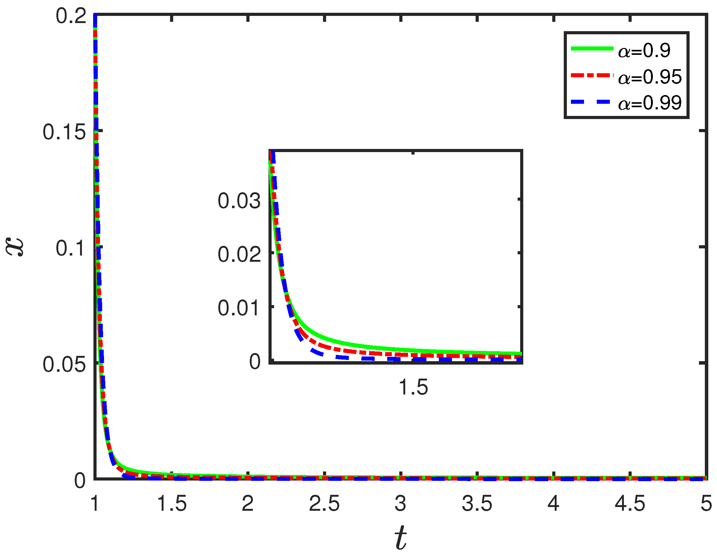
5. Numerical Examples

Now, we provide two examples to show the usefulness of the LDM for Hadamard-type systems. The predictor–corrector algorithm in [44] is employed for the numerical simulation.

Example 1.

Consider the following Caputo–Hadamard system:

$$\begin{array}{c}\hfill {}_{CH}{\mathrm{D}}_{1,t}^{\alpha }x\left(t\right)=-30x\left(t\right)-x^3\left(t\right),\end{array}$$

(76)

where $x\left(t\right)\in \mathbb{R}$.

The Lyapunov function is chosen as $W(t,x\left(t\right))=\frac{1}{2}{x}^2\left(t\right)$. Then,

$$\begin{array}{c}\hfill {}_{CH}{\mathrm{D}}_{t_0,t}^{\alpha }W(t,x)\le x{}_{CH}{\mathrm{D}}_{t_0,t}^{\alpha }x=x(-30x-x^3)\le -30{\parallel x\parallel }_2^2.\end{array}$$

(77)

As can be seen from (77) and Theorem 8, $x_e=0$ of the system (76) is HML stable. The corresponding curves in Figure 1 illuminate the stability clearly.

Example 2.

Consider the following Caputo–Hadamard system:

$$\begin{array}{c}\hfill \left\{\begin{array}{c}{}_{CH}{\mathrm{D}}_{1,t}^{\alpha }{x}_1=-2x_1-x_{2}sin\left(t\right)+3x_{3}cos\left(t\right),\hfill \\ {}_{CH}{\mathrm{D}}_{1,t}^{\alpha }{x}_2=x_{1}sin\left(t\right)-4x_2-2x_3,\hfill \\ {}_{CH}{\mathrm{D}}_{1,t}^{\alpha }{x}_3=-3x_{1}cos\left(t\right)+2x_2-5x_3,\hfill \end{array}\right.\end{array}$$

(78)

where $\alpha =0.98$.

Choosing the Lyapunov function

$$\begin{array}{c}\hfill W(x_1,x_2,x_3)=\frac{1}{2}{x}_1^2\left(t\right)+\frac{1}{2}{x}_2^2\left(t\right)+\frac{1}{2}{x}_3^2\left(t\right).\end{array}$$

Now, applying Remark 1, it can be found that

$$\begin{array}{cc}\hfill {}_{CH}{\mathrm{D}}_{t_0,t}^{\alpha }W(x_1,x_2,x_3)& =\frac{1}{2}{}_{CH}{\mathrm{D}}_{t_0,t}^{\alpha }{x}_1^2+\frac{1}{2}{}_{CH}{\mathrm{D}}_{t_0,t}^{\alpha }{x}_2^2+\frac{1}{2}{}_{CH}{\mathrm{D}}_{t_0,t}^{\alpha }{x}_3^2\hfill \\ \hfill & \le x_1{}_{CH}{\mathrm{D}}_{t_0,t}^{\alpha }{x}_1+x_2{}_{CH}{\mathrm{D}}_{t_0,t}^{\alpha }{x}_2+x_3{}_{CH}{\mathrm{D}}_{t_0,t}^{\alpha }{x}_3\hfill \\ \hfill & =x_1(-2x_1-x_{2}sin\left(t\right)+3x_{3}cos\left(t\right))+x_2(x_{1}sin\left(t\right)-4x_2-2x_3)\hfill \\ \hfill & +x_3(-3x_{1}cos\left(t\right)+2x_2-5x_3)\hfill \\ \hfill & =-2x_1^2-4x_2^2-5x_3^2\hfill \\ \hfill & \le -2x_1^2-2x_2^2-2x_3^2\hfill \\ \hfill & =-{2\parallel x\left(t\right)\parallel }_2^2.\hfill \end{array}$$

According to Theorem 8, $x_e=0$ of the system (78) is HML stable. Figure 2 just illustrate this result.

6. Conclusions

A class of Lyapunov theorems has been developed for non-linear Hadamard-type fractional systems. Additionally, several useful Hadamard-type fractional inequalities are investigated. Based on these inequalities, it is very easy to design a appropriate Lyapunov function and calculate their Hadamard-type fractional derivative. According to the modified Laplace transform and the properties of Hadamard fractional calculus, the asymptotic stability theories of Hadamard-type systems are discussed, which enriched the knowledge of fractional calculus. Using these results, LDM can be applied to analyze the HML stability of Hadamard-type systems. At last, two examples are given to check the results of the systems by using the developed theory. In the future, we may focus on the following meaningful topics:

• Extend the fractional order $\alpha$ of Hadamard-type system (38) and (39) from $(0,1)$ to $(1,2)$;
• Develop the asymptotic stability on incommensurate systems, switching systems, and time-delay systems;
• Choose appropriate Lyapunov functions for Hadamard-type system from a certain set.

References

1. Kilbas, A.A.; Srivastava, H.M.; Trujillo, J.J. Theory and aAplications of Fractional Differential Equations; Elsevier: Amsterdam, The Netherlands, 2006. [Google Scholar]
2. Rahimy, M. Applications of fractional differential equation. Appl. Math. Sci. 2010, 4, 2453–2461. [Google Scholar]
3. Dai, H.; Chen, W.S. New power law inequalities for fractional derivative and stability analysis of fractional order systems. Nonlinear Dyn. 2017, 87, 1531–1542. [Google Scholar] [CrossRef]
4. Sabatier, J.; Agrawal, O.P.; Machado, J.A.T. Advances in Fractional Calculus; Springer: Berlin/Heidelberg, Germany, 2007. [Google Scholar]
5. Uchaikin, V.V. Fractional Derivatives for Physicists and Engineers; Springer: Berlin/Heidelberg, Germany, 2013. [Google Scholar]
6. Li, Z.M.; Ma, W.; Ma, N.R. Partial topology identification of tempered fractional-order complex networks via synchronization method. Math. Methods Appl. Sci. 2021. [Google Scholar] [CrossRef]
7. Hu, T.C.; Li, L.L.; Wu, Y.Q.; Sun, W.G. Consensus dynamics in noisy trees with given parameters. Mod. Phys. Lett. B. 2022, 36, 2150608. [Google Scholar] [CrossRef]
8. İlhan, E. Analysis of the spread of Hookworm infection with Caputo-Fabrizio fractional derivative. Turkish J. Sci. 2022, 7, 43–52. [Google Scholar]
9. Ma, W.Y.; Li, Z.M.; Ma, N.R. Synchronization of discrete fractional-order complex networks with and without unknown topology. Chaos 2022, 32, 013112. [Google Scholar] [CrossRef] [PubMed]
10. Podlubny, I. Fractional Differential Equations; Academic Press: Cambridge, MA, USA, 1999. [Google Scholar]
11. Li, C.P.; Deng, W.H. Remarks on fractional derivatives. Appl. Math. Comput. 2007, 187, 777–784. [Google Scholar] [CrossRef]
12. Anatoly, A.K. Hadamard-type fractional calculus. J. Korean. Math. Sos. 2001, 38, 1191–1204. [Google Scholar]
13. Gong, Q.Z.; Qian, D.L.; Li, C.P.; Guo, P. On the Hadamard Type Fractional Differential System, Fractional Dynamics and Control; Springer: New York, NY, USA, 2012. [Google Scholar]
14. Katugampola, U.N. A new approach to generalized fractional derivatives. Bull. Math. Anal. Appl. 2014, 6, 1–15. [Google Scholar]
15. İlknur, K.; Akcetin, E.; Yaprakdal, P. Numerical approximation for the spread of SIQR model with Caputo fractional order derivative. Turk. J. Sci. 2020, 5, 124–139. [Google Scholar]
16. Akdemir, A.O.; Butt, S.I.; Nadeem, M.; Ragusa, M.A. New general variants of Chebyshev type inequalities via generalized fractional integral operators. Mathematics 2021, 9, 122. [Google Scholar] [CrossRef]
17. Ma, N.R.; Ma, W.Y.; Li, Z.M. Multi-Model Selection and Analysis for COVID-19. Fractal Fract. 2021, 6, 120. [Google Scholar] [CrossRef]
18. Brandibur, O.; Kaslik, E. Stability Analysis for a Fractional-Order Coupled FitzHugh–Nagumo-Type Neuronal Model. Fractal Fract. 2022, 6, 257. [Google Scholar] [CrossRef]
19. Li, C.P.; Li, Z.Q. Stability and logarithmic decay of the solution to Hadamard-type fractional differential equation. J. Nonlinear Sci. 2021, 31, 1–60. [Google Scholar] [CrossRef]
20. Ahmad, B.; Alsaedi, A.; Ntouyas, S.K.; Tariboon, J. Hadamard-Type Fractional Differential Equations; Springer: Berlin/Heidelberg, Germany, 2017. [Google Scholar]
21. Garra, R.; Mainardi, F.; Spada, G. A generalization of the Lomnitz logarithmic creep law via Hadamard fractional calculus. Chaos Solitons Fractals 2017, 102, 333–338. [Google Scholar] [CrossRef] [Green Version]
22. Ma, L. On the kinetics of Hadamard-type fractional defferential systems. Fractals 2020, 23, 553–570. [Google Scholar]
23. Brandibur, O.; Kaslik, E. Stability properties of a two-dimensional system involving one Caputo derivative and applications to the investigation of a fractional-order Morris–Lecar neuronal model. Nonlinear Dyn. 2017, 90, 2371–2386. [Google Scholar] [CrossRef] [Green Version]
24. Li, Y.; Chen, Y.Q.; Podlubny, I. Stability of fractional-order nonlinear dynamic systems: Lyapunov direct method and generalized Mittag-Leffler stability. Comput. Math. Appl. 2010, 59, 1810–1821. [Google Scholar] [CrossRef] [Green Version]
25. Liu, S.; Li, X.Y.; Jiang, W.; Zhou, X.F. Mittag-Leffler stability of nonlinear fractional neutral singular systems. Commun. Nonlinear Sci. Numer. Simul. 2012, 17, 3961–3966. [Google Scholar] [CrossRef]
26. Duarte-Mermoud, M.A.; Aguila-Camacho, N.; Gallegos, J.A. Using general quadratic Lyapunov functions to prove Lyapunov uniform stability for fractional order systems. Commun. Nonlinear Sci. Numer. Simul. 2015, 22, 650–659. [Google Scholar] [CrossRef]
27. Deng, W.H.; Li, C.P.; Lü, J.H. Stability analysis of linear fractional differential system with multiple time delays. Nonlinear Dyn. 2007, 48, 409–416. [Google Scholar] [CrossRef]
28. Liu, S.; Wu, X.; Zhou, X.F. Asymptotical stability of Riemann-Liouville fractional nonlinear systems. Nonlinear Dyn. 2016, 86, 65–71. [Google Scholar] [CrossRef]
29. Liu, S.; Wu, X.; Zhou, X.F. Asymptotical stability of Riemann-Liouville fractional singular systems with multiple time-varying delays. Appl. Math. Lett. 2017, 65, 32–39. [Google Scholar] [CrossRef]
30. Ma, L.; Wu, B. Finite-time stability of Hadamard fractional differential equations in weighted Banach spaces. Nonlinear Dyn. 2022, 107, 3749–3766. [Google Scholar] [CrossRef]
31. Hadamard, J. Essai sur l’étude des Fonctions, Données par Leur Développement de Taylor; Gauthier-Villars: France, French, 1892. [Google Scholar]
32. Jarad, F.; Baleanu, D.; Abdeljawad, A. Caputo-type modification of the Hadamard fractional derivatives. Adv. Differ. Equ. 2012, 2012, 142. [Google Scholar] [CrossRef] [Green Version]
33. Ma, L. Comparison theorems for Caputo-Hadamard fractional differential equations. Fractals 2019, 27, 1950036. [Google Scholar] [CrossRef]
34. Li, C.; Li, Z.; Wang, Z. Mathematical analysis and the local discontinuous Galerkin method for Caputo-Hadamard fractional partial differential equation. J. Sci. Comput. 2020, 85, 41. [Google Scholar] [CrossRef]
35. Wen, X.J.; Wu, Z.M.; Lu, J.G. Stability analysis of a class of nonlinear fractional-order systems. IEEE Trans. Circuits Syst. II Express Briefs. 2008, 55, 1178–1182. [Google Scholar] [CrossRef]
36. Chen, G.S. A generalized Young inequality and some new results on fractal space. Automatica 2012, 1, 56–59. [Google Scholar]
37. Aguila-Camacho, N.; Duarte-Mermoud, M.A.; Gallegos, J.A. Lyapunov functions for fractional order systems. Commun. Nonlinear Sci. Numer. Simul. 2014, 19, 2951–2957. [Google Scholar] [CrossRef]
38. Ding, D.S.; Qi, D.L.; Wang, Q. Non-linear Mittag–Leffler stabilisation of commensurate fractional-order non-linear systems. IET Control Theory Appl. 2015, 9, 681–690. [Google Scholar] [CrossRef]
39. Fernandez-Anaya, G.; Nava-Antonio, G.; Jamous-Galante, J.; Muñoz-Vega, R.; Hernández-Martínez, E. Lyapunov functions for a class of nonlinear systems using Caputo derivative. Commun. Nonlinear Sci. Numer. Simul. 2017, 43, 91–99. [Google Scholar] [CrossRef]
40. Wang, G.T.; Pei, K.; Chen, Y.Q. Stability analysis of nonlinear Hadamard fractional differential system. J. Franklin. Inst. 2019, 356, 6538–6546. [Google Scholar] [CrossRef]
41. Corduneanu, C. Principles of Differential and Integral Equations; American Mathematical Soc.: Providence, RI, USA, 2008. [Google Scholar]
42. Li, Y.; Chen, Y.Q.; Podlubny, I. Mittag-Leffler stability of fractional order nonlinear dynamic systems. Automatica 2009, 45, 1965–1969. [Google Scholar] [CrossRef]
43. Khalil, H.K.; Grizzle, J.W. Nonlinear Systems; Prentice Hall: Hoboken, NJ, USA, 2002. [Google Scholar]
44. Gohar, M.; Li, C.P.; Yin, C.T. On Caputo-Hadamard fractional differential equations. Int. J. Comput. Math. 2020, 97, 1459–1483. [Google Scholar] [CrossRef]
Figure 1. The evolution of system (76) with x ( 1 ) = 0.2 .
Fractalfract 06 00405 g001
Figure 2. The evolution of system (76). (a) x ( 1 ) = ( 1.2 , 1 , 1.5 ) T ; (b) x ( 1 ) = ( 1.2 , 1 , 1.5 ) T .
Fractalfract 06 00405 g002
Publisher’s Note: MDPI stays neutral with regard to jurisdictional claims in published maps and institutional affiliations.