Abstract
Vortex rope is a common phenomenon in the draft tube of hydraulic turbines. It may cause strong pressure pulsation, noise, and strong vibration of the unit especially when it is helical. Therefore, the study of vortex rope is of great significance. In order to study the helical vortex rope, the embedded large eddy simulation (ELES) method in the hybrid methods is used based on the vortex rope generator case. The Liutex method can show the three-dimensional shape of the vortex rope well. In order to quantitatively describe the helical vortex rope, the three-dimensional structure is divided into multiple two-dimensional sections, and then the shape of vortex rope on each section is processed to extract the perimeter and area of the vortex. Combined with the change trend of vortex number and section area, the helical vortex rope is divided into four zones. Then, the fractal dimension on each zone and section can be obtained, and it can be used to quantitatively analyze the change trend of the vortex rope in time and space. The fractal analysis method can be applied to the analysis of the vortex rope in the draft tube to help judge the flow pattern shape and the stability of the unit operating conditions.
1. Introduction
Vortex rope often occurs in the draft tube of hydro-turbines far away from the best operating efficiency, leading to various kinds of instabilities (e.g., large pressure fluctuation [1,2], significant noise, prominent vibrations [3], cavitation erosion [4], and material fatigue). The eccentric helical vortex rope frequency is generally about 1/4 to 1/3 of the rotating frequency of the runner [5]. To prevent structural vibration and increase the operation hours under off-design conditions, it is very important to understand the helical vortex rope structure in the draft tube fully. However, the accurate visualization with quantitative description of the detailed characteristics of vortex structure is a challenging task.
Several attempts were made to capture the vortices’ structures in the hydro-turbines. In order to study the effect of the flow rate on the vortex in the draft tube, Minakov et al. [6] used pressure iso-surface and Q criterion to visualize the vortices in the draft tube. Their results indicated that the guide vane opening has a significant effect on the distribution of vortices. Liu et al. [7] proposed the new Omega method (new Ω method), which is not sensitive to the threshold selection and can successfully capture both strong and weak vortices simultaneously. However, the Ω method has some limitations, such as the introduction of the uncertain parameter epsilon ε [8]. The Liutex method provides the systematic and mathematical definition of local rigid body rotation of fluid, and the related method is defined as the third-generation vortex identification method [9]. Tran et al. [10] applied Liutex method to identify the vortex rope of turbine-99’s off conditions and validated the reliability of identification for vortex rope.
The quantitative description of the vortex rope by its edge line requires the image processing of its two-dimensional section. The image segmentation can be divided into some non-overlapping sub-regions with their own characteristics, and each region is a continuous set of pixels, where the characteristics can be the color, shape, gray scale, and texture of the image. Image segmentation represents the image as a set of physically meaningful connected regions according to the prior knowledge of target and background. That is, the target and background in the image are marked and positioned, and then the target is separated from the background [11]. By using this method, the characteristics of vortices on a two-dimensional section can be extracted and the spatial distribution of vortices can be described quantitatively.
The fractal dimension of the vortex can be calculated by using the characteristics of the vortex extracted from image processing. The fractal dimension, D, has been used to study different properties of clouds. More than three decades ago, Lovejoy [12] reported D = 1.35 ± 0.05 for cloud and rain areas. Motivated by the seminal work of Lovejoy [12], Batista [13], Sánchez et al. [14], Luo and Liu [15], Von Savigny et al. [16], and Brinkhoff et al. [17] used the fractal analysis for clouds. The vortex rope in the two-dimensional section is very similar to the satellite captured clouds, where we can apply the fractal analysis to vortex rope. The above studies are all for cyclone motion in meteorology, the fractal dimension can predict the motion of cyclones, rarely in the application of vortex ropes in turbine draft tube. In this study, we analyze the relationship between the change of morphology and fractal dimension during the development of vortex rope, which can be used to analyze and predict the development of vortex rope.
In this study, the vortex rope generator is taken as an example. The turbulence model used in this paper is the embedded large eddy simulation (ELES) in the hybrid methods. All domains are first defined as the SST k-ω model, and then the draft tube domain is designated as wall-modeled LES (WMLES). The CFD results are compared with prior scholars’ experiment [18,19], and the three-dimensional structure of the helical vortex rope is identified and visualized by Liutex method. The Liutex method shows the three-dimensional structure of the vortex rope, and then the geometric parameters required to obtain the fractal corresponding to the Liutex contour-line of the vortex rope in two-dimensional sections. The characteristics of the vortex rope in two-dimensional sections are extracted by image segmentation technology, then the fractal dimension of the vortex rope is calculated, and the distribution and variation of the helical vortex rope in time and space are quantitatively described. According to the fractal analysis method proposed in this study, it can be applied to the analysis of the vortex rope in the hydraulic turbine draft tube to help determine the shape of the flow pattern and operational stability.
2. Research Subject
The size of the vortex rope generator is the same as the experimental model of Bosioc and Susan Resiga [18,19]. As shown in Figure 1, it consists of an inlet pipe, 13 fixed guide vanes, a runner with 10 blades, and a draft tube. The device is specially used to reproduce the vortex rope in the draft tube of a Francis turbine under part load, and its parameters are listed in Table 1. The flow rate is kept at 30 L s−1, the rotating speed of the runner is 920 r min−1. The inlet and outlet diameters are 0.15 m. The throat of draft tube is located below the runner nozzle with a radius of 0.05 m. The cross-section area of the draft tube increases gradually from the throat and remains constant until the exit. The distance from the runner nozzle to the draft tube outlet is 0.324 m. W2 on the right of Figure 1 is the measurement line of experiment applying laser Doppler velocimetry (LDV).
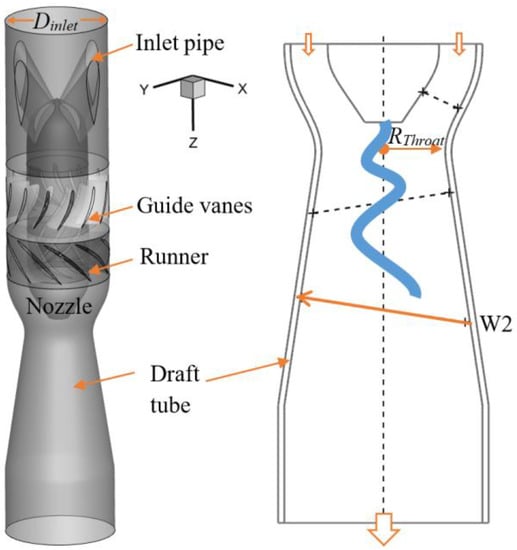
Figure 1.
Schematic of the swirl generator and position of velocity measured using laser Doppler velocimetry (LDV).

Table 1.
Parameters of the swirl generator.
3. Mathematical Methods
3.1. Turbulence Model
The CFD Vision 2030 Study [20] published by NASA indicates that the RANS-LES hybrid method will be widely used in the future. The Global RANS/LES hybrid method, represented by the detached eddy simulation (DES_ [21] has made great progress since it was proposed in 1997. By modifying the traditional turbulence model, the detached eddy simulation can automatically divide the RANS zone and LES zone according to the turbulence length scale and different spacing rate of the grid. The wall is modeled by RANS to reduce the amount of calculation. The main flow region is transformed from RANS model equation to the sub-lattices model, which significantly reduces the turbulence viscosity and plays a similar effect to LES implicit filtering. An inherent defect of the RANS/LES hybrid method is that the interface between RANS and LES is not controllable. Moreover, the interface does not modify the interaction information between the two zones. In particular, the large turbulence viscosity in the RANS zone directly enters the LES zone, severely inhibiting the analytical ability of the LES zone to turbulence and delaying the development of turbulence, namely the gray region problem [22]. An intuitive solution is to add appropriate turbulence pulsation at the interface, so that the flow from the RANS zone into the LES zone is transformed from a modular quantity to an analytical quantity, and the length of gray region is greatly shortened. In view of this, the embedded LES (ELES) method [23] came into being. Different from the global hybrid method, the embedded hybrid method needs to embed the LES zone into the RANS zone of the whole field in advance, and the interface between the RANS and LES zone is as perpendicular to the flow direction as possible to ensure the consistency of the flow direction and the information transfer direction from RANS to LES. In this way, additional turbulence information can be introduced at the interface more reasonably and conveniently to promote the further downstream development of turbulence in LES zone. This method is especially suitable for some local fine flow simulations with relatively simple geometry. The research object of this study is the helical vortex rope in the draft tube. It takes time and effort to apply LES to the overall domain, and the daft tube is a component downstream of the device, so it is suitable to apply the embedded hybrid method. Compared with LES, the ELES method can greatly shorten the computation period and alleviate the gray region problem in the Global RANS/LES hybrid method while ensuring the accuracy. Therefore, the ELES method is used to conduct the numerical simulation of the vortex rope generator in this study. The draft tube is set as the LES zone, and the other upstream domains set as the RANS zone. SST k-ω model suitable for fluid machinery is selected in the whole field, and wall-modeled LES (WMLES) is used in the LES zone. The WMLES model avoids the requirement of wall grid y+ = 1 in LES, which can further save the calculation time.
3.2. Fractal Dimension
For a geometric figure, dimension is an important characteristic quantity. Objects in Euclidean geometry are described in integer dimension, also known as topological dimension, and are represented by Dt. The Koch curve is either infinite or zero if measured on traditional integer dimensions (such as one and two dimension). This indicates that the Koch curve is not a regular geometric object and may have dimension between one and two. Only by measuring it with the scale of non-integer dimension can it accurately reflect its irregularity and complexity. The dimension of such non-integer value is called fractal dimension. Generally, the fractal dimension of a fractal curve is between one and two, and the larger the fractal dimension is, the more complex the curve is and the more it tends to fill the whole plane [24].
There are a multitude of methods to calculate fractal dimension in fractal geometry, some of which are classical, such as self-similarity dimension and box-counting dimension. To meet the needs of research, many other algorithms have evolved from the classical algorithm, such as area-perimeter method, root mean square method, and structural function method. In the study of a vortex, a single or group of irregular island patterns are often encountered, which are called fractal islands. The vortex rope has its edge line close to the regular shape of a circle or ellipse. These features are suitable for the area-perimeter method to calculate the fractal dimension of the vortex, so this study uses the area-perimeter method to calculate the fractal dimension of the vortex. There are two ways to determine fractal dimension according to the area-perimeter relationship of fractal island:
- Based on the perimeter, the filling degree of the perimeter of the fractal island in the plane is measured to determine the fractal dimension of the perimeter;
- Based on the area, the filling degree of the fractal island itself in the plane is used to measure the integral dimension of the surface.
These two methods can be used to determine the average fractal dimension (Da) of islands. However, the perimeter fractal dimension of slender island measured by this method will be high, and so will the area fractal dimension be calculated for nearly circular islands. The research object of this study is the two-dimensional graph of the vortex rope in the draft tube, whose shape is almost circular or elliptical. The boundary fractal dimension is used to describe the evolution process of vortex rope in time and space quantitatively.
The determination of perimeter fractal dimension is based on the relationship between the perimeter and the area of the fractal island, and its mathematical expression is as follows:
where P is the perimeter length of the outer edge line of a circle or ellipse, A is the area, D is the fractal dimension of the outer edge line, and k is the scale constant. Measure the perimeter and area of each island separately, and for a single island, its perimeter fractal dimension is:
For the vortices images, the average of vortex fractal dimensions (Da) can be determined by the slope obtained from the logarithmic plot of area and perimeter. Dm represents the main vortex fractal dimension, the main vortex is the biggest vortex on the 2D sections.
Compared with integer dimensions, fractal dimensions can more accurately reflect the occupation of space by objects. The fractal dimension describes the dynamic change of geometric figures, while it describes the correlation of the whole system behavior formed by small and fragmentary local features in natural phenomena. The fractal dimension can be used to describe the correlations between small vortices and large vortices, and to discuss the relationship between the structures of various scale vortices.
4. Computational Fluid Dynamics Simulation
4.1. Boundary Conditions and Modeling Setups
Commercial solver ANSYS Fluent is used for present studies. Velocity inlet and pressure outlet are set in the simulation. No slip velocity conditions are used at the walls. The speed of runner n is set as 920 r min−1. The temperature field is considered with the initial value of 300 K. The ELES model is used to account for turbulence effects. The process of setting ELES in ANSYS Fluent is as follows: first, set the all domain as SST k-ω turbulence model, then specify the turbulence model in the draft tube domain as WMLES which belongs to LES method, and then set the interface between RANS domain and LES domain. In the simulation, the time step is 1/360 revolution (i.e., 1 degree rotation at a single time step). A total of 10,800 time steps is calculated. The steady state solution is obtained after 1800 time-steps, and we start data sampling for time statistics after 3600 time-steps.
Basic Equations
Filtering the continuity and momentum equations, one obtains
where is the stress tensor, and is the subgrid-scale stress.
The subgrid-scale (SGS) stresses resulting from the filtering operation are unknown and require modeling. The subgrid-scale turbulence models in Ansys Fluent employ the Boussinesq hypothesis [25] as in the RANS models, computing subgrid-scale turbulent stresses from
where μt is the subgrid-scale turbulent viscosity. As for incompressible flows, the term involving τkk can simply be neglected [26]. is the rate-of-strain tensor for the resolved scale.
The Algebraic WMLES formulation was proposed in the works of Shur et al. [27]. It combines a mixing length model with a modified Smagorinsky model [28] and with the wall-damping function of Piomelli [29].
In the Shur et al. model [27], the eddy viscosity is calculated with the use of a hybrid length scale:
where dw is the wall distance, S is the strain rate, κ = 0.4187 and CSmag = 0.2 are constants, and y+ is the normal to the wall inner scaling.
The LES model is based on a modified grid scale to account for the grid anisotropies in wall-modeled flows:
Here, hmax is the maximum edge length for a rectilinear hexahedral cell. hwn is the wall-normal grid spacing, and Cw = 0.15 is a constant.
Temperature transport equation:
Equation (8) is, from left to right, the transient term representing the net increase rate of controlling body temperature, the convective term representing temperature with fluid flow rate, the diffusion term representing the net diffusion rate of controlling body due to diffusion, and the source term representing other effects, which is zero herein.
4.2. Verification of Mesh Resolution and Mesh Convergence
In the CFD simulation, the flow domains need to be discretized. Grid size is of great importance for the accuracy of numerical results. The coarse grid cannot get enough turbulent information while a much too refined grid requires unaffordable computational cost. It is necessary to make a good compromise between accuracy and computational cost.
In order to obtain the enough detailed information of vortex rope, it is necessary to evaluate the LES region’s grid quality. Celick [30] developed a method to extrapolate and analyze the LES region’s grid quality by turbulent kinetic energy k. The LES Index of Quality (LES_IQ), indicating the percentage of directly resolved turbulent kinetic energy kres in LES, can be employed to evaluate the quality of grid. Pope [31] suggests that the 80% of the energy should be resolved everywhere for LES. If the LES_IQ is greater than 80%, we consider it a good LES. This study uses this method to estimate the sensitivity of the grid resolution quality. The grid detail is show in Table 2. Figure 2 shows a detailed view of the section mesh on the X-Z section in the swirl generator. Each domain adopts hexahedral structure grids.
Table 2.
Grid details.
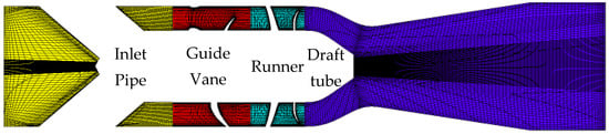
Figure 2.
Mesh details on X-Z section.
The LES_IQ can be calculated with Equation (9) for the fine grid and Equation (10) for the coarse grid.
Fine grid index:
Coarse grid index:
where and represents the resolved turbulent kinetic energy of fine grid and coarse grid, urmse, vrmse, and wrmse are velocity components’ Root Mean Squared Error. The order of accuracy of the numerical scheme p is 2 and α = (ΔxΔyΔz)c/(ΔxΔyΔz)f1/3 = 1.35 is grid refinement parameter, in which Δx, Δy, and Δz are the grid cell lengths in the three directions.
kres = 1/2(urmse2 + vrmse2 + wrmse2)
Figure 3 shows the turbulent kinetic energy and LES_IQ resolved by two sets of grids on line W2 and the turbulent kinetic energy of fine mesh is significantly higher than coarse mesh. The LES_IQ of the fine mesh is greater than 90%, while the coarse mesh is low to 65%. It is obvious that the solution accuracy of the fine mesh is much higher than the coarse mesh. The fine mesh is more abundant for the flow field details. Therefore, all subsequent analyses use the CFD results of the fine mesh.
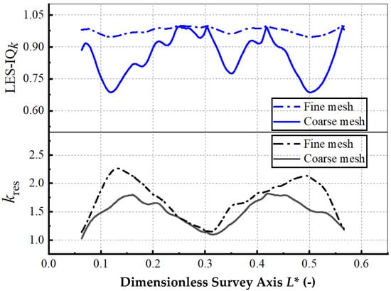
Figure 3.
Turbulent kinetic energy and LES_IQ of two sets of grids on W2. (L* = LW2/Rthroat, where LW2 is the length of Line W2.)
4.3. Comparison between Experiment and Numerical Simulation
Figure 4 shows the comparison between ELES method simulation and LDV experiment. The axial velocity of ELES in the middle region is greater than that of the experiment result in LDV. The reason is that there is a reverse flow near the center due to the gas phase in the vortex rope. However, pure water medium is used in the simulation, and the axial velocity direction of the fluid always points to the outlet. The tangential velocity of ELES is basically consistent with the experimental results. The results of comparison show that the simulation results can be used for further analysis.
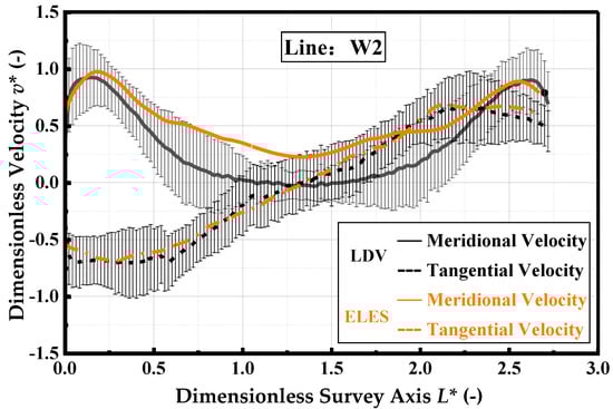
Figure 4.
The velocity comparison between simulation and experiment. (v* = v/vthroat, where v is axial velocity or tangential velocity).
4.4. Comparison of Vortex Rope Morphology in Different Vortex Recognition Method
The Q criterion [32] and new Ω method [7] in the second-generation method, and Liutex method in the third-generation method are selected to compare the shape of vortex rope in the draft tube. Figure 5 shows that the vortex structures displayed by the three vortex identification methods are roughly the same. There are some wall-attached vortices identified by Q criterion in the throat, and it is difficult to remove through threshold selection. When the Ω method is under construction, different ε is selected in the denominator, and the vortex structure shows different results when Ω = 0.52. It relies on experience to debug the value of ε, and belongs to the second-generation vortex identification method, so the shear term cannot be removed [9,10]. From Figure 4, the vortex structure displayed by the Liutex method is clearer than that of the Ω method because the shear term in the vorticity is removed by the Liutex method, which makes the displayed vortex cleaner and less polluted by shear. l* is Liutex magnitude. Therefore, in this study, the Liutex method is used to display vortex rope morphology in the draft tube and further analysis.
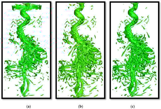
Figure 5.
The morphology of vortex rope identified by three vortex identification methods at a certain moment. (a) Q = 200,000 s−1; (b) Ω = 0.52; (c) l* = 500 s−1.
5. Analysis of Time-Space Fractal Dimension of Vortex Rope
5.1. Analysis Method of Coarse Granulation
The graph in Figure 6a is the output graph of one section of the draft tube, and such multi-contour-lines graph can be regarded as the description of ‘fine-grained’. Considering that the focus of this study is the fractal structure of vortex or vortex block contour line, the analysis method of coarse-grained is used instead of fine-grained. That is, when the graph is output, the details of contour distribution inside the vortex are ignored, and only the contour line of the vortex (described by MLTX = 50) is given. Considering that the focus of the analysis in the paper is the fractal structure of vortex contour lines, the analysis method of coarse-grained is used instead of fine-grained. In other words, when outputting the graphs, only the vortex contour lines are given without considering the details of the vortex internal contour distribution. This coarse-grained description can make the focus prominent and the graphical display clear and intuitive. The dimensionless relative Liutex magnitude MLTX given by , ω is angular velocity of runner. The coarse-grained variation corresponding to Figure 6a is shown in Figure 6b. Here, we trace how the shape of the contour lines shown in Figure 6b evolve over time and space, without considering other various issues that are not directly related to fractals, such as the central strength of the vortex rope or how the asymmetric structure changes over time. The contour line of MLTX = 50 represents the edge line of the vortex rope. This coarse-grained description can highlight the key points and make the graphic displayed clearer and more intuitive.
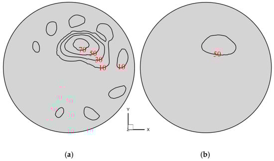
Figure 6.
Relative Liutex magnitude MLTX on one section of the draft tube. (a) Fine-grained description; (b) Coarse-grained description. (The numbers represent relative Liutex magnitude).
5.2. Contour Line Evolution
5.2.1. Spatial Evolution of Vortex Tube Contour Lines
The distance from the runner nozzle to the outlet is 0.324 m. In order to observe the morphological changes of the vortex rope in the process of spiraling downstream, the runner nozzle to the outlet of the draft tube is divided into 33 sections with an interval of 10 mm, as shown in Figure 7. MLTX = 50 is used to show the three-dimensional structure of the vortex rope. The vortex rope is more concentrated when it is close to the draft tube and presents different forms as the vortex rope spins downstream. In order to facilitate observation, the vortex rope on the two-dimensional section was coarsely grained. After the processing, the vortex rope on the two-dimensional section was generally in the shape of a single island. As the vortex rope extended downstream, it began to break and became an archipelago in section. After the cross-sectional area of the draft tube stopped increasing, the vortex rope began to gather again and the number of islands decreased significantly.
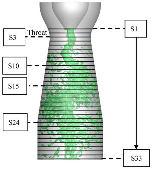
Figure 7.
Schematic diagram of different sections of vortex rope in draft tube.
Figure 8 is a schematic diagram of the image processing process on a 2D section of one draft tube section resulting from numerical simulation at a certain moment. The specific operation is as follows: the output section vortex graph is binarized (the gray value of the points on the image is 0 or 255), that is, the whole image presents an obvious black and white effect. Brinkhoff et al. [19] extensively analyzed the influence of holes in images for the first time, and concluded that in most cases, clouds containing holes meant an increase in fractal dimension. Remove holes by morphological image processing (open operation and close operation: open operation can remove isolated small points, and the overall position and shape is unaltered; the close operation can fill in small lakes (i.e., small holes) and close small cracks), while the position and shape remain unchanged. Finally, each vortex on the section is marked, and then the parameters such as circumference and area of each vortex are calculated to prepare for the calculation of fractal dimension in the next step.
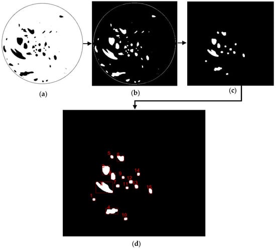
Figure 8.
Schematic diagram of image processing process on a 2D section of draft tube. (a) Original image; (b) binarization processing; (c) morphological operation (open operation and closed operation); (d) mark vortex.
The number of vortices on each section can also be obtained by marking. Figure 9 shows the number of vortices on each section for an instance. At the section near the runner nozzle, the vortex rope is a complete spiral vortex rope. From S10, the number of vortices begins to increase until it reaches a peak at S15. The vortex rope oscillates more violently than its gathering ability, making it unable to maintain its shape and breaking up on a large scale between S15 and S24. After S24, as the section area does not increase any more, the vortex rope begins to gather again. However, the energy of the vortex rope at this time has been greatly dissipated, so the straight vortex rope re-formed near the outlet is small and accompanied by a slice of secondary vortices.
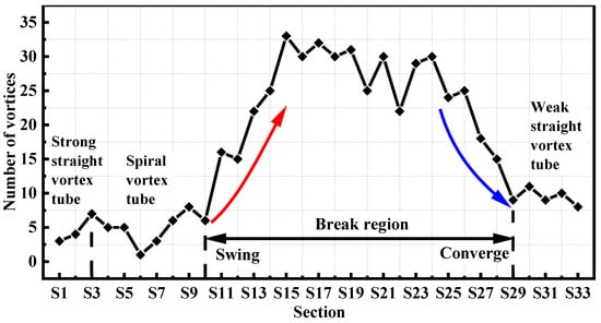
Figure 9.
The number of vortices in each section.
Figure 10 shows the distribution of vortex ropes in each section after treatment. The section close to the runner nozzle shows that there are several secondary vortices stretched by the wall around the main vortex. Before the S3 section of the throat, the vortex rope is always in the center position. After passing through the throat, the secondary vortices near the vortex rope decrease and begin to rotate eccentrically downstream. From S4 to S10, it is a spiral vortex rope. After S10, the vortex rope begins to break, and the degree of breakage reaches the peak at S15. In the section of S15–S24, the breakage is always at a high level. There is no obvious main vortex on the sections between S10 and S27, but a vortex cluster composed of broken vortices rotates around the central axis. At the beginning of S24 section, the number of vortices begins to decrease as the cross-section area of the draft tube no longer increases. The main vortex rope reappeared in the center of S29 cross section, and the broken vortices gradually decrease. As the section here is far from the energy source of the vortex rope (vortex at the impeller outlet), the energy transferred to the straight pipe section can only form the thin straight vortex rope downstream as shown in Figure 7. According to the shape and number of vortices, the draft tube is divided into four regions: strong straight vortex rope zone (S1–S3), spiral vortex rope zone (S4–S10), broken vortex rope zone (S10–S29), and weak straight vortex rope zone (S29–S33).
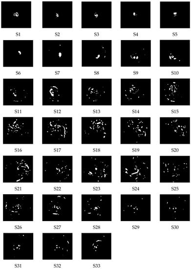
Figure 10.
Vortex distribution on each section after morphological operation.
The vortex rope has obvious eccentricity and precession in the process of downstream development, and with the increase of the cross-section area, the eccentricity becomes stronger and stronger until the cross-section area stops increasing and converges again into a straight vortex rope. The strength of the straight vortex rope is obviously weakened compared with that of the spiral vortex rope initially located at the runner nozzle. The flow loses energy when flowing through the expanding section. When the vortex rope is in the expanding tube, there also exists an obvious energy loss. The helical action on the plane will tear the vortex rope, and with the downward spiral, this trend becomes more obvious. The vortex rope is torn from a nearly circular shape into a crescent shape and further into fragments. Figure 10 shows that the large-scale vortex in the fracture zone is stretched into a crescent shape. The small vortex is easily affected by shear force, and its shape becomes more and more round. The shear action of fluid causes the large-scale vortex to break and the small-scale vortex to get round.
Table 3 shows the perimeter fractal dimension of vortex rope on each section calculated according to Equation (2). The main vortex refers to vortices whose area is significantly larger than other vortices on the same section. Combined with Figure 11, the Da of all sections except S1 is less than or equal to main vortex fractal dimension (Dm). The Dm of each section in the strong straight vortex rope zone ranges from 1.38 to 1.5, and Dm ranges from 1.25 to 1.56. The Da of each section in the spiral vortex rope zone ranges from 1.31 to 1.39, and Da ranges from 1.10 to 1.24. The Dm of each section in the broken vortex rope zone is between 1.33 and 1.46, and the Da is between 1.13 and 1.27. The Dm of each section in the weak straight vortex rope zone ranged from 1.35 to 1.47, and the Da ranged from 1.09 to 1.35.
Table 3.
Main vortex fractal dimension (Dm) or average fractal dimension (Da) of vortex rope on each section.
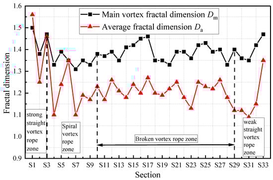
Figure 11.
Fractal dimensions of vortex rope on each section.
As the vortex rope rotates downstream, its degree of eccentricity increases obviously, the number of secondary vortices also gradually increases, and the overall Da decreases gradually. According to the statistical results, on the same section, the dimension of the main vortex is the smallest, and Da is smaller than Dm. To some extent, fractal dimension can be used to represent the size and shape of vortex.
Figure 12 shows the fractal dimension relation of all vortices’ circumferences and areas on the sections of the draft tube, expressed in logarithmic coordinates. The logarithmic relation of all samples is fitted by the following linear relation:
where C0 is 0.2836 and C1 is 0.6099. The Da of the vortex rope is 1.2066. Figure 12 shows Da of the four zones. Linear fitting of logarithmic relationship is performed in the form of Equation (6), and the values of C1 and C0 are obtained as shown in Table 4. Figure 13 shows Da of each zone. According to the calculation, the Da of the strong straight vortex rope zone is 1.4454, that of the spiral vortex rope zone is 1.1698, that of the broken vortex rope zone is 1.2180, and that of the weak straight vortex rope zone is 1.1916.
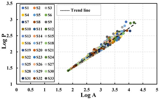
Figure 12.
Fractal dimension relation of all vortices’ circumferences and areas on the sections of the draft tube.
Table 4.
Dimensions of peripherals of vortices in different zones.
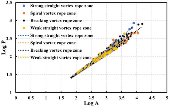
Figure 13.
Fractal dimension relation of vortex circumferences and areas in four zones of draft tube.
5.2.2. Temporal Evolution of Vortex Tube Contour Lines
In the previous section, the spatial evolution process of the vortex rope at a certain moment was discussed and the vortex rope was quantified by fractal dimensions. However, there is a large randomness in a single moment, so it is necessary to observe the shape of the vortex rope at different moments and record the dimension changes of the cross-section and partition.
The impeller rotation of 1/8 revolution was taken as the time interval to observe the changes of vortex rope morphology in the draft tube and compare the changes of vortex rope at eight continuous moments.
Figure 14 shows the shape changes of vortex rope. The vortex rope still maintains four zones at different moments. Special sections of the strong straight vortex rope zone near the runner nozzle, the spiral vortex rope zone where the vortex rope starts to spiral, the broken vortex rope zone and the weak straight vortex rope zone, namely sections S3, S9, S19, and S29, were taken to observe the dimensional changes of the four sections at different moments. Figure 15 shows the changes of shape at different moments on the four special sections. At most of the moments, the shape of the vortex rope is similar. The vortex rope rotates about the central axis on S3. The vortex rope is crescentic on S9, and it is seriously eccentric with several secondary vortices. In the section of S19, the vortices still rotate around the central axis after being completely broken. In the section of S29, there is always a vortex at the center and some secondary vortices revolve around it. This shows that the morphology of vortex rope basically does not change over time.
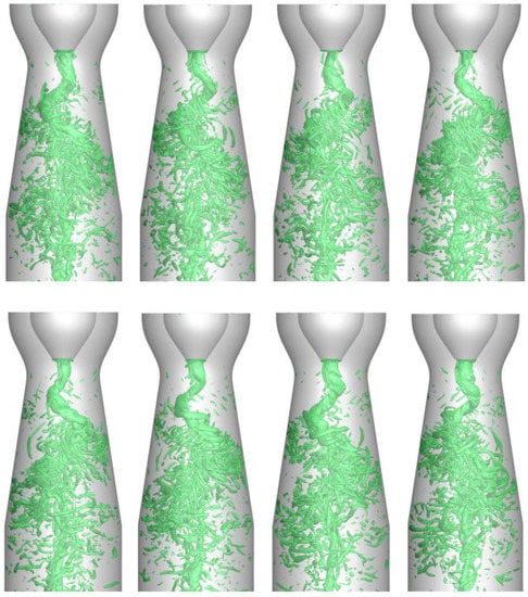
Figure 14.
Shape of vortex rope at eight continuous moments.
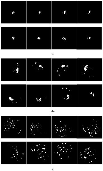
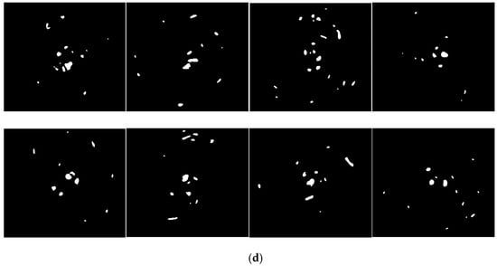
Figure 15.
Vortex shape on four special sections at eight moments. (a) Vortex shape on S3 at eight moments; (b) Vortex shape on S9 at eight moments; (c) Vortex shape on S19 at eight moments; (d) Vortex shape on S29 at eight moments.
Figure 16 is the comparison of Da at eight moments on four special sections. The results show that Da in different zones has a certain size law, but it also changes with time. Figure 16a shows the Da of vortex on four special sections at eight continuous moments. The Da of S3 is the largest and the Da of S29 is the smallest. From the Figure 16b listed, it can be seen that the Da of S9 representing the spiral vortex rope zone changes greatly over time compared with the other three zones. The spiral vortex rope zone is vulnerable to the impact of axial flow, resulting in the instability of the spiral vortex rope zone, the boundary between the spiral vortex rope zone and the broken vortex rope zone is not obvious, resulting in a large change in Da. Figure 16c shows that the Da of four zones decreases gradually as the vortex rope spiral downstream. The vortex rope upstream of S9 maintains its own morphology and the vortex rope downstream of S9 breaks up. The vortex rope at the S9 section is at the position of the strongest oscillation and may maintain its own morphology at different moments or may have broken up, resulting in a large range of variation in the fractal dimension of the S9 section at different moments. By judging the pulsation amplitude of the fractal dimension, we can determine where the vortex rope starts to break up. The fractal dimensions are relatively stable in other sections and do not fluctuate much.
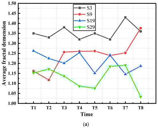
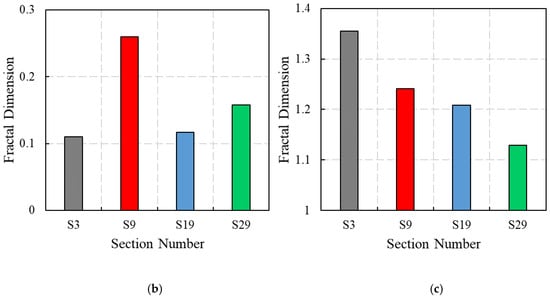
Figure 16.
Comparison of Da at eight moments on four special sections. (a) Da at eight continuous different moments on four special sections; (b) Maximum-minimum difference of Da; (c) Average value of Da.
6. Conclusions
Based on computational fluid dynamics and ELES method, this study accurately simulates the helical vortex rope and studies its fractal characteristics. The conclusions are as follows:
- For the helical vortex rope, which is a typical vortex dominated flow, different vortex identification methods have different effects. In this study, the Liutex method was selected to identify the vortex structure of the helical vortex rope and display the three-dimensional shape of vortex rope. The helical vortex rope was divided into different sections. Through binarization and morphological operation, the vortices at different positions can be quantified. This method can be extended to the vortex flow of hydraulic machinery to deeply analyze the characteristics and evolution of vortices.
- Based on the analysis of different sections, the number and fractal dimension of vortices were obtained. Combined with the change trend of vortex number and section area, the distribution area of the helical vortex rope was divided into four zones, namely strong straight vortex zone, spiral vortex zone, broken vortex rope zone, and weak straight vortex zone. The Da of each section and zone is counted by the least square method, and the fractal characteristics of vortex rope in space are quantitatively analyzed, which has a good effect on the analysis of the formation, fragmentation, and reunion of vortex rope. It was found that in the process of spiraling downstream, the shape of the vortex rope develops from a strong straight vortex rope near the runner nozzle to a weak straight vortex rope at the outlet, the Da decreases gradually, and the vortex rope in the middle is always spiraling downward whether it is broken or not.
- Because the results at a single time are random, the variation trend of fractal dimension of each section and zone with time was analyzed. The results show that Da in different zones has a certain size law, but it also changes with time. According to the difference between the average value and the maximum minimum difference of Da at eight times of the runner rotation, it can be found that the average of Da in the strong straight vortex rope zone is the largest and the maximum minimum difference of Da is the smallest. The maximum minimum difference in the spiral vortex rope zone is the largest. The average and maximum minimum difference of Da at the broken vortex rope zone are relatively small. The average value of Da at weak straight vortex zone is the smallest, and the maximum minimum difference of Da is relatively large.
The forms of vortex ropes that often appear in the operation of hydro turbine or marine turbine are mainly divided into two categories: straight vortex rope and helical vortex rope. According to the fractal analysis method proposed in this study, it can be applied to the analysis of the vortex rope flow in the draft tube of hydraulic turbines to help judge the flow pattern shape and the operation stability.
Author Contributions
Conceptualization, R.T. and P.L.; writing—original draft preparation, P.L. and S.Y.; writing—review and editing, P.L. and R.T.; supervision, R.X. and D.Z. All authors have read and agreed to the published version of the manuscript.
Funding
This research was funded by the Open Research Fund Program of State Key Laboratory of Hydroscience and Engineering (No. sklhse-2022-E-01) and National Natural Science Foundation of China (No. 52079142 and 51836010).
Institutional Review Board Statement
Not applicable.
Informed Consent Statement
Not applicable.
Data Availability Statement
Data available on request from the corresponding author.
Conflicts of Interest
The authors declare no conflict of interest.
References
- Chen, T.; Zhang, Y.; Li, S. Instability of large-scale prototype Francis turbines of three gorges power station at part load. Proc. Inst. Mech. Eng. Part A J. Power Energy 2016, 230, 619–632. [Google Scholar] [CrossRef]
- Zhang, Y.; Chen, T.; Li, J.; Yu, J. Experimental study of load variations on pressure fluctuations in a prototype reversible pump turbine in generating mode. ASME J. Fluids Eng. 2017, 139, 074501. [Google Scholar] [CrossRef]
- Xu, H.Q.; Wang, F.J.; Meng, L.; Liao, C.; Liu, Z.; Wang, W.; He, L. Discussion about the mechanism of self-excited arcuate cyclotron of Francis turbine shaft. Larg. Electr. Mach. Hydraul. Turbine 2022, 2, 55–62. [Google Scholar]
- Zhang, Y.; Zhang, Y.; Qian, Z.; Ji, B.; Wu, Y. A review of microscopic interactions between cavitation bubbles and particles in silt-laden flow. Renew. Sustain. Energy Rev. 2016, 56, 303–318. [Google Scholar] [CrossRef]
- Rheingans, W.J. Power swings in hydroelectric power plants. Trans. ASME 1940, 62, 171–184. [Google Scholar]
- Minakov, A.V.; Platonov, D.V.; Dekterev, A.A.; Sentyabov, A.V.; Zakharov, A.V. The analysis of unsteady flow structure and low frequency pressure pulsations in the high-head Francis turbines. Int. J. Heat Fluid Flow 2015, 53, 183–194. [Google Scholar] [CrossRef]
- Liu, C.; Wang, Y.; Yang, Y.; Duan, Z. New omega vortex identification method. Sci. China Phys. Mech. Astron. 2016, 59, 1–9. [Google Scholar] [CrossRef]
- Dong, X.R.; Wang, Y.Q.; Chen, X.; Dong, Y.; Zhang, Y.N.; Liu, C. Determination of epsilon for omega vortex identification method. J. Hydrodyn. 2018, 30, 541–548. [Google Scholar] [CrossRef]
- Liu, J.; Liu, C. Modified normalized Rortex/vortex identification method. Phys. Fluids 2019, 31, 061704. [Google Scholar] [CrossRef]
- Tran, C.T.; Long, X.-P.; Ji, B.; Liu, C. Prediction of the precessing vortex core in the Francis-99 draft tube under off-design conditions by using Liutex/Rortex method. J. Hydrodyn. 2020, 32, 623–628. [Google Scholar] [CrossRef]
- Shi, J.B.; Malik, J. Normalized cuts and image segmentation. IEEE Trans. Pattern Anal. Mach. Intell. 2000, 22, 888–905. [Google Scholar] [CrossRef]
- Lovejoy, S. Area-perimeter relation for rain and cloud areas. Science 1982, 216, 185–187. [Google Scholar] [CrossRef] [PubMed]
- Batista-Tomás, A.R.; Díaz, O.; Batista-Leyva, A.J.; Altshuler, E. Classification and dynamics of tropical clouds by their fractal dimension. Q. J. R. Meteorol. Soc. 2016, 142, 983–988. [Google Scholar] [CrossRef]
- Sánchez, N.; Alfaro, E.J.; Pérez, E. The fractal dimension of projected clouds. Astrophys. J. 2005, 625, 849–856. [Google Scholar] [CrossRef]
- Luo, Z.; Wang, Y.; Ma, G.; Yu, H.; Wang, X.; Sao, L.; Li, D. Possible causes of the variation in fractal dimension of the perimeter during the tropical cyclone Dan motion. Sci. China Earth Sci. 2014, 57, 1383–1392. [Google Scholar] [CrossRef]
- Savigny, C.V.; Brinkhoff, L.A.; Bailey, S.M.; Randall, C.E.; Russell, J.M. First determination of the fractal perimeter dimension of noctilucent clouds. Geophys. Res. Lett. 2011, 38, L02806. [Google Scholar] [CrossRef]
- Brinkhoff, L.A.; Savigny, C.V.; Randall, C.E.; Burrows, J.P. The fractal perimeter dimension of noctilucent clouds: Sensitivity analysis of the area–perimeter method and results on the seasonal and hemispheric dependence of the fractal dimension. J. Atmos. Sol.-Terr. Phys. 2015, 127, 66–72. [Google Scholar] [CrossRef]
- Susan-Resiga, R.; Muntean, S.; Tanasa, C.; Bosioc, A.I. Hydrodynamic design and analysis of a swirling flow generator. In Proceedings of the 4th German–Romanian Workshop on Turbomachinery Hydrodynamics (GRoWTH), Stuttgart, Germany, 12–15 June 2008. [Google Scholar]
- Bosioc, A.; Susan-Resiga, R.; Muntean, S. 2D LDV Measurements of swirling slow in a simplified draft tube. In Proceedings of the Conference on Modelling Fluid Flow CMFF, Budapest, Hungary, 9–12 September 2009. [Google Scholar]
- Slotnick, J.; Khodadoust, A.; Alonso, J.; Darmofal, D.; Gropp, W.; Lurie, E.; Mavriplis, D.J. CFD Vision 2030 Study: A Path to Revolutionary Computational Aerosciences; NASA/CR2014-218178R; NASA: Hampton, VA, USA, 2014.
- Strelets, M. Detached eddy simulations of massively separated flows. In Proceedings of the 39th Aerospace Sciences Meeting and Exhibit, Reno, NV, USA, 8–11 January 2011. [Google Scholar]
- Wilcox, D.C. Turbulence Modeling for CFD, 3rd ed.; DCW Industries Inc.: La Cañada, CA, USA, 2006. [Google Scholar]
- Davidson, L.; Peng, S. Embedded large-eddy simulation using the partially averaged navier-stokes model. AIAA J. 2013, 51, 1066–1079. [Google Scholar] [CrossRef]
- Mandelbrot Benoit, B. The fractal geometry of nature. Am. J. Phys. 1998, 51, 468. [Google Scholar] [CrossRef]
- Erlebacher, G.; Hussaini, M.Y.; Speziale, C.G.; Zang, T.A. Toward the large-eddy simulation of compressible turbulent flows. J. Fluid Mech. 1992, 238, 155–185. [Google Scholar] [CrossRef]
- Shur, M.L.; Spalart, P.R.; Strelets, M.K.; Travin, A.K. A hybrid RANS-LES approach with delayed-DES and wall-modelled LES capabilities. Int. J. Heat Fluid Flow 2008, 29, 1638–1649. [Google Scholar] [CrossRef]
- Hinze, O. Turbulence; McGraw-Hill Publishing, Co.: New York, NY, USA, 1975. [Google Scholar]
- Smagorinsky, J. General circulation experiments with the primitive equations. I. The basic experiment. Mon. Weather. Rev. 1963, 91, 99–164. [Google Scholar] [CrossRef]
- Piomelli, U.; Moin, P.; Ferziger, J.H. Model consistency in large-eddy simulation of turbulent channel flow. Phys. Fluids 1988, 31, 1884–1894. [Google Scholar] [CrossRef]
- Celik, I.B.; Cehreli, Z.N.; Yavuz, I. Index of resolution quality for large eddy simulations. J. Fluids Eng. 2005, 127, 949–958. [Google Scholar] [CrossRef]
- Pope, S.B. Turbulent Flows; Cambridge University Press: Cambridge, UK, 2000; Volume 12, p. 806. [Google Scholar]
- Da Silva, C.B.; Pereira, J.C.F. Invariants of the velocity-gradient, rate-of-strain, and rate-of-rotation tensors across the turbulent/nonturbulent interface in jets. Phys. Fluids 2008, 20, 055101. [Google Scholar] [CrossRef] [Green Version]
Publisher’s Note: MDPI stays neutral with regard to jurisdictional claims in published maps and institutional affiliations. |
© 2022 by the authors. Licensee MDPI, Basel, Switzerland. This article is an open access article distributed under the terms and conditions of the Creative Commons Attribution (CC BY) license (https://creativecommons.org/licenses/by/4.0/).