Numerical Investigation on Effective Elastic Modulus of Multifractal Porous Materials

Abstract

The design of a novel material necessitates a fundamental understanding of its structure–property relation. Inorganic porous materials (media) such as natural soil and rock, and artificial ceramic and cement, exhibit multifractal characteristics in view of their structural heterogeneity. This paper presents a numerical investigation of the effective elastic modulus of multifractal porous materials. Two types of deterministic and stochastic cascading algorithms are employed to synthesize the multifractal fields, and then a mathematical formula is proposed to perform the conversion from the intensity of a multifractal field to the local elastic modulus of a multifractal porous material. Furthermore, a finite element method is used to achieve the homogenization of the local elastic modulus. Special attention is paid to the dependence of the effective elastic modulus on the structural heterogeneity of multifractal porous materials.

1. Introduction

An essential part of material research is developing a fundamental understanding of the structure–property relation [1]. It is believed that such a basic relation could provide theoretical guidance for the design of novel materials from structure modification to property optimization [2,3]. In practice, inorganic materials (media) such as natural soil and rock and artificial ceramic and cement have very complex internal structures, i.e., irregular fractures and pores are dispersed within a solid matrix. For such porous materials, the structure–property relation depends not only on the solid matrix, but also on the pore network [4].

A variety of experimental techniques have been applied to investigate the structural features of porous materials, including gas adsorption, mercury intrusion porosimetry (MIP), small-angle neutron scattering (SANS), scanning electron microscopy (SEM), X-ray-computed tomography (XCT), and nuclear magnetic resonance (NMR) tests. Each has its own advantages and drawbacks, as documented in detail [5,6,7,8,9,10,11,12]. Meanwhile, some advanced theories have been proposed to describe the structural heterogeneity from a mathematical viewpoint, such as fractal self-similarity and multifractal statistics [13]. Using these, the structural heterogeneity may be defined as the quality or diversity of certain characteristics. More specifically, porous materials (media) are represented by the level of dissimilarity of pore-space, the pore and throat size distribution, the tortuousness of their connections and their spatial distribution. Fractals refer to broken or fractured geometric patterns with a shared feature called self-similarity. That can be understood by the analogy of zooming into a digital image to uncover its finer structure; if this is done on a fractal, no new details appear, i.e., nothing changes and the same pattern repeats over and over. Fractal self-similarity shows great advantages related to its concise mathematics, i.e., a universal power law relationship accounts for the scale-dependent structure. Nevertheless, the reality is more complex, since one often finds that most objects and phenomena tend to deviate from a perfect fractal. In comparison to fractals, the term multifractal describes objects or phenomena consisting of multiple fractals that depend on the scale or region of interest. As a matter of fact, the multifractal statistic has proven itself as a valuable tool for describing complex systems with chaotic and nonlinear dynamics, and therefore highly irregular structural features. Instead of the single fractal dimension discussed in the fractal theory, a group of multifractal parameters, such as the Rényi dimension, the Hölder exponent and the multifractal spectrum, provide some good options for a quantitative measurement of the structural heterogeneity within multifractal theory.

The application of multifractal statistics to inorganic porous materials, including soil, rock, ceramic and cement, has undergone fast developments and contributed useful results over the years. For instance, San José Martínez et al. investigated the representative elementary area (REA) of soil space, i.e., the minimum area of a soil block section that was required to represent the features of interest, in terms of the entropy dimension of the pore network [14]. Soto–Gómez et al. used the multifractal spectrum to characterize the scaling properties of the pore network in soil as the statistical descriptors of its topology, and even to correlate the macroscopic physical properties, such as the transport and retention of substances through it [15]. Guan et al. compared the multifractal parameters among shales, through which the multifractal statistic was demonstrated as a promising tool for the quantitative evaluation of the internal complexity of heterogeneous rocks [16]. Duan et al. compared the multifractal characteristics of deeply buried carbonate rocks, and introduced two multifractal parameters as the indicators of pore structure types via case studies [17]. Stach et al. carried out the multifractal statistic analysis of stereometric files obtained from a confocal microscope and achieved high efficiency in detecting the locations of pores on an alumina ceramic coating surface [18]. Dănilă et al. implemented the multifractal statistic to achieve the reliable separation of replicas from genuine ceramics belonging to the Cucuteni–Tripolye culture, as the relative rarity of genuine examples has led to a flood of fake (replica) archeological artefacts in the marketplace [19]. Valentini et al. used the multifractal spectrum extracted from digital images of cement paste as a structural probe to determine the tendency of calcium silicate hydrate gel to form clusters [20]. Gao et al. adopted the width of the singularity spectrum as the index to quantify the structural heterogeneity, and further investigated its effect on the elastic modulus of ordinary Portland cement paste [11,21].

In practice, several methods can be used for the analysis of the multifractal statistic, which can be divided into two classes, i.e., box-counting methods and others based on wavelets. For the first class, the space of interest needs be meshed with a certain number of identical boxes, and a normalized measure is computed for each box [22,23]. The second class is based on the wavelet transform, and there is here no need to mesh the space of interest [24,25]. In contrast to the abundance of analysis tools, only a few works have proposed actual algorithms for the generation or synthesis of the multifractal statistic, particularly in controllable scaling exponents. To date, as inspired by canonical binomial cascades, multiplicative cascades have always played a central role in generating multifractals [26,27]. For instance, Perfect et al. described the synthesis of a multifractal Sierpinski carpet based on multipliers composed of average mass fractions calculated from the truncated two-parameter binomial distribution [28]. Cheng proposed a five-parameter binomial multiplicative cascade, which permitted the synthesis of an asymmetrical multifractal [29]. These attempts all relied on a deterministic algorithm, i.e., the same multipliers were used through the cascading process. Besides this, some stochastic algorithms have been put forward by means of the incorporation of random multipliers during the cascading process. For instance, Barral and Mandelbrot introduced the multifractal products of cylindrical pulses, i.e., the compound Poisson cascades, and recognized their rigorous multifractal characteristics [30]. By prescribing the correlation function of the increments of a random walk, Muzy and Bacry developed the multifractal random walk algorithm [31]. Chainais formulated compound Poisson cascades as well as infinitely divisible cascading noise, motion and random walk in a general framework, and provided strong results regarding convergence and scaling behavior [32,33].

As one of the fundamental parameters controlling mechanical properties, the elastic modulus has been broadly studied in terms of the porosity–modulus relation in porous materials. Much earlier, Hashin and Shtrikman proposed the widely used upper and lower bounds for the effective elastic moduli of a macroscopically homogeneous and isotropic composite material of an arbitrary phase geometry [34]. Such formulae were able to provide a good estimate for the effective moduli, assuming the ratios between the different phase moduli were not too large, i.e., the bounds derived were sufficiently close. Budiansky and O’connell calculated the elastic moduli of bodies containing randomly distributed flat cracks based on a self-consistent method, wherein general concepts were outlined for arbitrary cracks and explicit derivations were given for elliptic cracks [35]. Zhao et al. considered porous materials with spherical pores of given distributions, and derived the five independent elastic constants for each arrangement by means of Mori–Tanaka’s mean field theory in conjunction with the Eshelby’s solution [36]. Gong et al. applied a stepped equivalent substitution approach to extend the Mori–Tanaka model to predicting the elastic behavior of porous materials, whereby the effects of pore size, pore number and sample size were taken into account [37]. Manoylov et al. examined the details of several models used for the prediction of elastic characteristics of natural and synthetic porous materials, and then introduced an extended Vavakin–Salganik model for those composed of isolated spherical pores with various statistical distributions [38]. Making use of finite element modeling, Chen et al. calculated the elastic modulus of porous ceramic films fabricated by constrained sintering, wherein the microstructure was reconstructed from focused ion beam/scanning electron microscope (FIB/SEM) tomography [39]. It was concluded that porosity was the key variable that controlled the elastic modulus of the partially sintered ceramic films, while other features of the microstructure, such as the pore size, had only a minor influence. Some other relevant work can be found in Grigorenko et al. [40], Abbas and Zenkour [41], Abbas [42] and Dyyak et al. [43]. Note that most previous attempts have been concentrated on the dependence of the elastic modulus on the overall porosity, pore shape and pore size distribution. Nevertheless, the usage of such parameters, i.e., the overall porosity, pore shape and pore size distribution, might be insufficient or inappropriate for describing the complexity of a realistic pore network, particularly for multifractal porous materials. Balankin proposed the concept of multifractal elasticity for the prediction of the mechanical behaviors of multifractal materials, and derived a closed system of constitutive equations on the basis of two phenomenological laws of reversible deformations of multifractal structures [44]. Thereafter, to the best of our knowledge, progress related to a general investigation of the elastic characteristics for multifractal porous materials remains sparse.

This paper presents a numerical investigation of the effective elastic modulus of multifractal porous materials, with special attention paid to the effect of structural heterogeneity. To that end, two types of deterministic and stochastic algorithms are employed to synthesize multifractal fields. A mathematical formula is proposed to account for the conversion from the intensity of a multifractal field to the local elastic modulus of a multifractal porous material, and a finite element method is implemented to compute the effective elastic modulus. The remainder of this paper is organized as follows: Section 2 presents a brief description of multifractal porous materials; Section 3 introduces two types of cascading algorithms, including the two-parameter binomial multiplicative cascade and the compound Poisson cascades; Section 4 describes the conversion from the intensity of a multifractal field to the local porosity and elastic modulus of a multifractal porous material; Section 5 focuses on the finite element method to achieve the homogenization of the elastic modulus; Section 6 gives the results and discussion.

2. Multifractal Porous Materials

The statistical properties of the structural heterogeneity of multifractal porous materials are often characterized by parameters such as the Rényi dimension, the Hölder exponent, and the multifractal spectrum. Depending on the experimental technique adopted, the specific multifractal parameters considered might differ in practice. For this,

Table 1. Previous works examining the multifractal characteristics of inorganic porous materials.

Authors	Porous Materials	Experimental Techniques	Multifractal Parameters
San José Martínez et al. (2007) [14]	Soils from central Spain	Confocal microscope, digital camera	Entropy dimension
Soto-Gómez et al. (2020) [15]	Soils from northwestern Spain	X-ray-computed tomography	Rényi dimension, multifractal spectrum
Guan et al. (2020) [16]	Lacustrine shales from the Bohai Bay Basin of China	Gas adsorption, mercury intrusion porosimetry	Rényi dimension, multifractal spectrum
Duan et al. (2021) [17]	Carbonate rocks from the Tazhong Uplift of China	Gas adsorption, mercury intrusion porosimetry, nuclear magnetic resonance	Capacity dimension, Hölder exponent
Stach et al. (2014) [18]	Al2O3 coating deposited on an aluminum alloy disc	Confocal microscope	Hausdorff dimension spectra
Dănilă et al. (2018) [19]	Ceramic pottery in Cucuteni–Tripolye culture	Scanning electron microscopy	Rényi dimension, multifractal spectrum
Valentini et al. (2012) [20]	Ordinary Portland cement	X-ray powder diffraction microtomography	Multifractal spectrum
Gao et al. (2021) [21]	Ordinary Portland cement	X-ray-computed tomography	Multifractal spectrum

gives an overview of some previous works regarding the examination of the multifractal characteristics of inorganic porous materials.

The Rényi dimension D_q (also called the generalized fractal dimension) is defined as [13]:

$$D_q=\underset{\delta \to 0}{lim}\frac{I_q\left(\delta \right)}{\mathit{ln}\delta }$$

(1)

$$I_q\left(\delta \right)=-\frac{1}{q-1}\mathit{ln}\left[{\displaystyle \sum }_{i=1}^{N\left(\delta \right)}{P}_i^q\left(\delta \right)\right]$$

(2)

$${\displaystyle \sum }_{i=1}^{N\left(\delta \right)}{P}_i\left(\delta \right)=1$$

(3)

I_q is the generalized entropy of order q, P_i (δ) is the probability (the normalized local porosity) of a point lying in the i-th box (element) used to cover the space of interest, and δ is the box size, which also represents the spatial scale. Some dimensions having explicit physical meanings include the capacity dimension D₀ for q = 0, the entropy (information) dimension D₁ for q = 1 and the correlation dimension D₂ for q = 2. As shown in Figure 1, the space of interest needs be meshed with a certain number of identical boxes for the first class of methods in an analysis of the multifractal statistic. Usually, a power series of spatial scales δ is chosen out of convenience.

Besides I_q, the generating or partition function χ_q (δ) is defined as [13]

$${\chi }_q\left(\delta \right)={\displaystyle \sum }_{i=1}^{N\left(\delta \right)}{P}_i^q\left(\delta \right)$$

(4)

For the multifractal statistic, χ_q (δ) exhibits a scaling behavior over a wide range of scales such that

$${\chi }_q\left(\delta \right)~{\delta }^{\tau \left(q\right)}$$

(5)

τ(q) is called the mass exponent, which is a nonlinear function of q [14].

For each box, the relation between the probability measure P(δ) and the scale δ can be expressed as

$$P\left(\delta \right)~{\delta }^{\alpha }$$

(6)

α is called the Hölder exponent, which characterizes the strength of a singularity [14]. Because of the fluctuation of P(δ) among different boxes, α is a continuous variable that is bounded within an interval. The number of boxes N(δ, α) with the same α satisfies

$$N\left(\delta ,\alpha \right)~{\delta }^{-f\left(\alpha \right)}$$

(7)

f (α) is called the Hausdorff dimension [15].

The multifractal parameters are not independent but correlated through [15]

$$\tau \left(q\right)=\left(q-1\right)D_q$$

(8)

$$\alpha =\frac{d\tau \left(q\right)}{dq}$$

(9)

$$f\left(\alpha \right)=q\alpha -\tau \left(q\right)$$

(10)

3. The Multiplicative Cascades Used for Synthesizing the Multifractal Fields

3.1. Paradigm of the Multiplicative Cascades

In practice, apart from the reconstructed microtomographic images providing a three-dimensional description, most microstructural information is two-dimensional, as obtained from direct images of various kinds, such as digital camera and microscope images. For this, the synthesis of multifractal porous materials prevails in the two-dimensional case, and thus this was also the case in the current study. The multiplicative cascades have always played a central role in the synthesis of multifractal fields [26]. The paradigm of a cascading process is illustrated in Figure 2. A dimensionless unit box (see n = 0) is divided into b² identical small ones of size 1/b (see n = 1), where b is the cascading resolution. Each sub-box is assigned a weight p_i ≥ 0 (i = 1, 2, …, b²). Then, this process is repeated. The small boxes of size 1/b are further divided into b² identical smaller ones of size 1/b², and the weights q_j ≥ 0 (j = 1, 2, …, b²) are assigned such that each smaller box has a weight p_iq_j (see n = 2). This is continued n times until the homogeneity scale (δ = 1/bⁿ) is reached, at which point each small box becomes homogeneous. In principle, the specific choice of the weights or multipliers (p_i, q_j, …) determines the type of the cascading process. That is, if the multipliers are kept the same through the cascading process, this is a deterministic algorithm; if the multipliers are independent but correlated at a given cascading level, this is a stochastic algorithm.

3.2. Two-Parameter Binomial Multiplicative Cascades

The classical Sierpinski carpet and its three-dimensional cousin (the Menger sponge) have a long history of applications in modeling pore and fracture networks in natural porous materials (media). It is well known in mathematics that they are strict fractals. Based on this, Perfect et al. described the synthesis of a multifractal Sierpinski carpet or Menger sponge, wherein the multipliers were assigned average mass fractions calculated from the truncated binomial distribution of two parameters [28]. In particular, let N = b², and the multipliers can be given as

$$p_i={\displaystyle \sum }_{k=0}^{i-1}B\left(N-k,N,p\right)\frac{1}{N-k}$$

(11)

B is the truncated binomial probability, written as

$$B\left(k,N,p\right)=\frac{\left(\frac{N!}{k!\left(N-k\right)!}\right)p^k{\left(1-p\right)}^{N-k}}{{{\displaystyle \sum }}_{k=1}^N\left(\frac{N!}{k!\left(N-k\right)!}\right)p^k{\left(1-p\right)}^{N-k}}$$

(12)

The values of p_i depend on the two critical parameters b and p. Figure 3 shows the variation of p_i with p for b = 4, which tends to be less steep when p → 1. The solid lines are used for the sake of clarity, and p_i is valid only at the discrete integers of i. The horizontal axis refers to i = 1…16, denoting the serial number of a sub-box. The vertical axis shows the values of the multipliers p_i. As mentioned above, when the cascading process is continued, the same multipliers {p_i} = {q_j} shall be used. Since p → 1 leads to a smaller discrepancy between the upper and lower bounds of p_i, i.e., 0.135 for p = 8/16 and 0.076 for p = 13/16, a rather homogeneous multifractal field can be anticipated. That is, the structural heterogeneity depends fully on b and p for the multifractal field generated by the two-parameter binomial multiplicative cascades.

For the two-parameter binomial multiplicative cascades of the deterministic algorithm, the generating function χ_q (δ = 1/bⁿ) is expressed as

$${\chi }_q\left(\frac{1}{b^n}\right)={\left(\frac{1}{b^n}\right)}^{\tau \left(q\right)}$$

(13)

Equation (13) has to be satisfied for any a cascading level (the times of repeating) n. Thus, setting n = 1 and substituting Equations (11) and (12) into Equation (13) gives the Rényi dimension as

$$\left\{\begin{array}{ll}{D}_q=\frac{1}{\left(1-q\right)\mathit{ln}b}\mathit{ln}\left[{\displaystyle \sum }_{i=1}^N{\left(p_i\right)}^q\right],& q\ne 1\\ D_1=-{\displaystyle \sum }_{i=1}^N{p}_i\mathit{ln}\left(p_i\right)/\mathit{ln}b,& q=1\end{array}\right.$$

(14)

3.3. Compound Poisson Cascades

The multiplicative cascades of the deterministic algorithm are computationally very easy to implement, but they have two major drawbacks. Their construction is not space shift-invariant, i.e., it is not strictly stationary. Besides this, the scaling behavior favors only the prescribed scale ratio equal to the given parameter b (integer ≥ 2). One of the solutions to both drawbacks is to replace the rigid nested arrangement of multipliers with some random ones generated in a marked Poisson point process (x, r, W) [32,33]. For this, the locations x are i.i.d. uniformly distributed on the real space with density 1; the scales r are i.i.d. random variables on (δ, 1) with a well-chosen probability; the marks or multipliers W are i.i.d. positive random variables. Such types of random multiplicative cascades are often called the compound Poisson cascades, since they are built as a combination of the Poisson point process of (x, r) and the random multiplier W. In particular, by introducing the space-scale cone of influence C_δ(x) = {(x^, r): δ ≤ r ≤ 1, ‖x^–x‖ < r/2}, the compound Poisson cascades give [32]

$$Q_{\delta }\left(x\right)=\frac{{{\displaystyle \prod }}_{\left(x_i,r_i\right)\in C_{\delta }\left(x\right)}{W}_i}{E\left[{{\displaystyle \prod }}_{\left(x_i,r_i\right)\in C_{\delta }\left(x\right)}{W}_i\right]}$$

(15)

Q_δ (x) accounts for the intensity of a multifractal field at the location x and the spatial resolution δ, and E denotes the mathematical expectation. Each realization of this random process could be regarded as a block taken from a different location of the multifractal porous material. The compound Poisson cascades have found many applications in the statistics of turbulent flows and natural images, since they are easy to synthesize numerically. The scaling exponent is described as E [Q_δ (x)^q] = δ^{φ (q)} with φ(q) = 1 − E (W^q) − q(1 − EW), or equivalently E [ε_δ(x)^q] = δ^{τ (q)}, where ε_δ (x) is the box average of Q_δ(x) over a ball of radius δ [33]

$${\epsilon }_{\delta }\left(x\right)=\frac{{{\displaystyle \int }}_{||x^-x||<\delta }Q\left(\mathrm{x}\text{^}\right)d\mathrm{x}\text{^}}{{{\displaystyle \int }}_{||x^-x||<\delta }d\mathrm{x}\text{^}}$$

(16)

In general, this satisfies φ (q) = τ (q), at least within some limited range of values of q [45]. Furthermore, for a particular family of the compound Poisson cascades, i.e., when the random multipliers have a probability density function G (W) = ζW^{(ζ − 1)} with ζ > 0 and W∈[0, 1], they depend on the parameter ζ only. Figure 4 shows the variations of G (W) for different values of ζ. The case ζ = 1 yields G (W) = 1, i.e., W is distributed uniformly in [0, 1]. Meanwhile, one can note that the probability of W approaching unity becomes much larger when ζ >> 1. If a random multiplier W → 1, the cascading process becomes W_iW → W_i. That is, as the cascading level n goes down, the structural heterogeneity will not be intensified. Therefore, for such a family of compound Poisson cascades, a fairly homogeneous multifractal field can be anticipated when ζ >> 1.

For these particular compound Poisson cascades, the Rényi dimension D_q takes the simple form of

$$D_q=d-\frac{q}{\left(\zeta +1\right)\left(\zeta +q\right)}$$

(17)

4. Conversion from the Intensity of a Multifractal Field to the Elastic Modulus

The intensity of a multifractal field g = p_i or Q_δ (x) can be normalized as:

$$f=\frac{g-g_{min}}{g_{max}-g_{min}}$$

(18)

or

$$f=\frac{g}{g_{max}}$$

(19)

g_min and g_max are the minimum and maximum values of g, respectively. Equations (18) and (19) are equivalent in most practices, since g_min tends to approach zero for the two types of multiplicative cascades. Such a linear transformation from g to f does not change the structural heterogeneity on one side; naturally, it takes the form 0 ≤ f ≤ 1, and f can thus be considered as the porosity of a porous material in general on the other side. As such, in the following sections, we define f as the local porosity of the synthesized multifractal porous materials.

A variety of empirical formulae have been proposed to account for the porosity–modulus relation of porous materials [46,47,48,49,50,51]. One such classical equation is written in terms of an exponential law:

$$E=E_0\mathit{exp}\left(-Af\right)$$

(20)

where E₀ is the zero-porosity elastic modulus, which depends on the solid matrix, and A is a parameter related to the pore network of the material [46,47]. Herein, the dependence of the Young’s modulus on porosity is demonstrated, while other forms of the elastic modulus can be described in a similar manner [52]. These typical relations were fitted from numerous sets of experimental data for different types of porous materials. Due to the complexity of real porous materials, such as the transition of the pore structure from interconnected to isolated, it is generally believed that A might not be constant for the entire range of porosity 0 ≤ f ≤ 1. Wang presented different physical models and discussed in detail the effects of pore neck geometry, particle size and grain growth, and the type of packing system, which could influence the value of A, i.e., A = 1.72, 3.37 and 5.02, as shown in Figure 5 [46]. In consequence, some nonlinear terms of f are often added to address the deviations of the porosity–modulus relation from the classical formula, such as the incorporation of high-order terms such as Af + Bf² [53]. According to Figure 5, it is not difficult to conclude that as the porosity f increases, the deviations become more drastic. The pure arithmetic fit in terms of the incorporation of high-order terms such as Af + Bf² will not result in a universal formula that can account for the porosity–modulus relation of a porous material. Therefore, differently from previous attempts, we point out that the parameter A can be viewed as a material constant for the entire range of porosity 0 ≤ f ≤ 1 if only the dimension of a porous material is small enough. Meanwhile, the deviations of the porosity–modulus relation from the classical formula can be attributed to the structural heterogeneity of realistic porous materials. For this, Equation (18) or Equation (19) can be substituted into Equation (20), which yields a mathematical formula accounting for the conversion from the intensity of a multifractal field g to the elastic modulus E, as:

$$E=E_0\mathit{exp}\left[-A\left(\frac{g-g_{min}}{g_{max}-g_{min}}\right)\right]$$

(21)

or

$$E=E_0\mathit{exp}\left[-A\left(\frac{g}{g_{max}}\right)\right]$$

(22)

5. Finite Element Method for the Homogenization of Elastic Modulus

The finite element method considers each isotropic element as having its own elastic modulus tensor. The essential idea is that a variational principle pertains for the linear elastic problem, i.e., the final distribution of strain satisfies the condition that the total elastic energy should be an extremum [54,55]. Using the Voigt notation of symmetry, the elastic energy Θ stored in each element is written as [54]

$$\mathsf{\Theta }=\frac{1}{2}{\epsilon }_l{E}_{lm}{\epsilon }_{m}dxdy$$

(23)

ε_l and ε_m are local strains at a point (x, y) within the element; l and m are labels covering the three components, i.e., l, m = 1, …, 3; E_lm is the local elastic modulus tensor. The algorithm reduces the energy equation to a quadratic form in terms of the nodal displacements.

As shown in Figure 6, the nodal displacement is written as u_rγ, where r (or s) = 1, …, 4 is the label covering the 4 nodes, and γ (or λ) = 1, 2 denotes the two components in a two-dimensional Cartesian coordinate system. Each component of the displacement is linearly interpolated across the element. As a result, the γ-th component of the displacement at a point (x, y), i.e., u_γ (x, y), is defined as

$$u_{\gamma }\left(x,y\right)=F_{\gamma ,r\lambda }\left(x,y\right)u_{r\lambda }$$

(24)

F_γ,rλ is the shape function for a square bi-linear element, i.e., F_γ,1λ = (1–x) (1–y), F_γ,2λ = x (1–y), F_γ,3λ = xy, and F_γ,4λ = (1–x) y if γ = λ; otherwise, F_γ,rλ = 0.

The local strain can be converted from the local displacement at point (x, y) as

$${\epsilon }_l\left(x,y\right)=S_{l,r\lambda }\left(x,y\right)u_{r\lambda }$$

(25)

The conversion function S is written as

$$S_{l,r\lambda }\left(x,y\right)=T_{l\gamma }{F}_{\gamma ,r\lambda }\left(x,y\right)$$

(26)

with T = (∂/∂x 0; 0 ∂/∂y; ∂/∂y ∂/∂x).

Substituting Equations (24)–(26) into the energy expression Equation (23) leads to [55]

$$\mathsf{\Theta }=\frac{1}{2}{[S_{l,r\gamma }{u}_{r\gamma }]}^T{E}_{lm}\left[S_{m,s\lambda }{u}_{s\lambda }\right]dxdy$$

(27)

Grouping the S and E matrices together, and performing the integral over the element with respect to the terms that have (x, y) dependence, yields

$$\mathsf{\Theta }=\frac{1}{2}{[u_{r\gamma }]}^T{\Psi }_{r\gamma ,s\lambda }\left[u_{s\lambda }\right]$$

(28)

with

$${\Psi }_{r\gamma ,s\lambda }={[S_{l,r\gamma }]}^T{E}_{lm}\left[S_{m,s\lambda }\right]dxdy$$

(29)

Ψ_rγ,sλ is the stiffness matrix. The global elastic energy must be summed over all elements, which is a large quadratic functional in terms of the nodal displacements. The variational principle requires that the gradient of elastic energy with respect to the nodal displacements is zero, which can be solved using a conjugate scheme. The effective strain <ε_l> and stress <σ_l> are then obtained using the average of each component of the strain tensor and stress tensor over all elements, such that

$$〈{\epsilon }_l〉=\frac{{\epsilon }_{l}dxdy}{dxdy}$$

(30)

$$〈{\sigma }_l〉=\frac{E_{lm}{\epsilon }_{m}dxdy}{dxdy}$$

(31)

< > denotes the averaging operator. Using the general Hooke’s law for an isotropic medium, the effective modulus tensor E_eff is solved using

$$〈{\sigma }_l〉=E_{\mathit{eff}}〈{\epsilon }_l〉$$

(32)

6. Results and Discussions

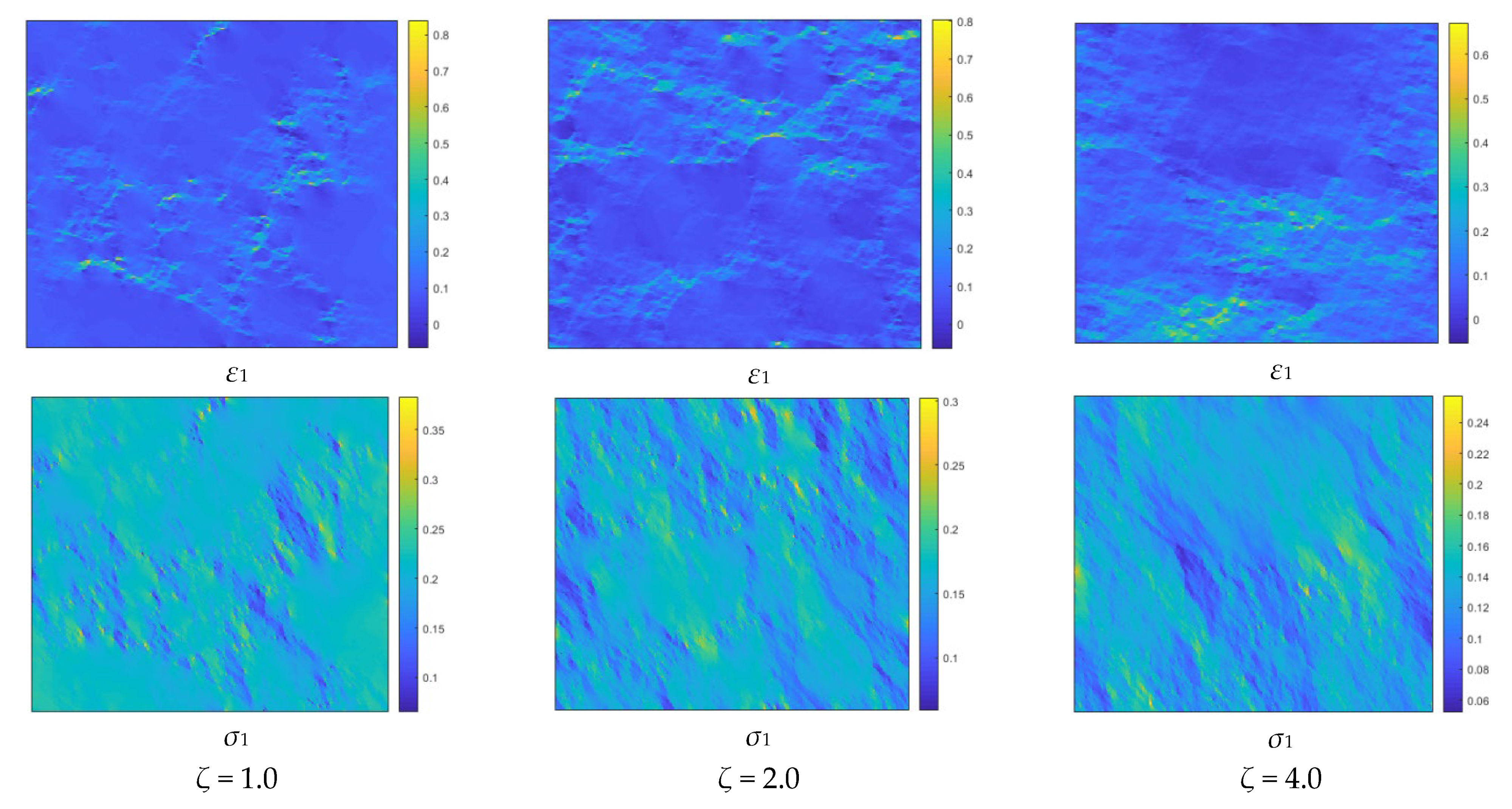
6.1. The Structural Heterogeneity of Multifractal Porous Materials

The examples in Figure 7 and Figure 8 show some digital images of the multifractal porous materials synthesized from the two-parameter binomial multiplicative cascades and the compound Poisson cascades. Each of these is 256 × 256 pixels (elements) in size. The grayscale of each pixel corresponds to a distinct local porosity f with 0 ≤ f ≤ 1. The higher the porosity, the darker the element. The multifractal porous materials (Figure 7) synthesized by the two-parameter binomial multiplicative cascades exhibit the highly regular patterns of a rigid hierarchy, which can be used to model fracture networks in soil and rock. Those images (Figure 8) synthesized by the compound Poisson cascades exhibit very random textures, which can be used to model pore networks in ceramic and cement. Moreover, when p → 1 (for the two-parameter binomial multiplicative cascades) or ζ >> 1 (for the compound Poisson cascades), one expects to observe rather homogeneous images with a lot of black regions associated with small values (f → 0), and some isolated white points associated with rare extreme values (f → 1).

Figure 9 presents the quantitative characterization of structural heterogeneity for the two-parameter binomial multiplicative cascades and the compound Poisson cascades. In particular, the Rényi dimension D_q is taken into account. Theoretically, for the given parameters (b, p) or ζ, if all the values of D_q are equal, a monofractal (strict fractal) is described. If, however, the values of D_q are different, a multifractal is then described. We define the range of D_q as ΔD = D₀ − D_+∞, where the capacity dimension D₀ = 2 equals the topological dimension 2 of the space, and D_+∞ is approximated by D₁₀. In essence, ΔD provides a quantification of the structural heterogeneity. That is, a highly clustered distribution is indicated by a higher value of ΔD compared to a randomly dispersed distribution, whereas the spectrum of a totally homogeneous distribution that fills the global domain reduces to a point, such that ΔD = 0. Perfect et al. demonstrated that for the two-parameter binomial multiplicative cascades, the multifractal scaling exponents were consistent at any q of (−∞, +∞) [28]. Lashermes et al., however, showed that the compound Poisson cascades could undergo systematic linearization—for a certain range of orders q, the estimate accounts correctly for the multifractal scaling exponents; outside this range, the estimate significantly departs from the correct values and behaves systematically as a linear function of q [45]. Figure 9 indicates that as p (from 8/16 to 13/16) and ζ (from 0.5 to 16) increase, the structural heterogeneity ΔD decreases in the two-parameter binomial multiplicative cascades (from 0.510 to 0.143) and the compound Poisson cascades (from 0.635 to 0.023), respectively.

6.2. Finite Element Method Used to Determine the Effective Elastic Modulus

Most importantly, each pixel (element) within the synthesized multifractal porous materials must be small enough, and therefore the classical porosity–modulus formula can be applied to compute the elastic modulus. Then, finite element computation can achieve the homogenization of the local elastic modulus, i.e., the determination of the effective elastic modulus E_eff/E₀. To that end, the classical Spriggs’ equation with A = 1.72 is used to account for the porosity–modulus relation, which does not compromise the generality. That is, E/E₀ = exp (−1.72f) is assumed for each pixel (element) when computing the two types of multifractal porous materials. The homogeneous engineering strains are imposed on each element initially, i.e., (ε₁, ε₂, ε₃) = (0.1, 0.1, 0.1). This accords with the preset rule that when the total elastic energy reaches an extremum, the final dimensionless strain (ε₁) and stress (σ₁) are recorded within multifractal porous materials. Figure 10 (for the two-parameter binomial multiplicative cascades) and Figure 11 (for the compound Poisson cascades) show maps of the dimensionless strain and stress. Then, homogenization of the elastic modulus is performed by means of the general Hooke’s law for an isotropic medium. The results are summarized in

Table 2. Macroscopic porosity <f> and effective elastic modulus E_eff/E₀ of multifractal porous materials synthesized by the two-parameter binomial multiplicative cascades.

Parameter	<f>	Eeff/E0	Error of Eeff/E0
b = 4, p = 8/16	0.046	0.904	0.019
b = 4, p = 9/16	0.080	0.848	0.023
b = 4, p = 10/16	0.128	0.776	0.031
b = 4, p = 11/16	0.197	0.692	0.035
b = 4, p = 12/16	0.289	0.592	0.029
b = 4, p = 13/16	0.409	0.484	0.021

and

Table 3. Macroscopic porosity <f> and effective elastic modulus E_eff/E₀ of multifractal porous materials synthesized by the compound Poisson cascades.

Parameter	<f>	Error of <f>	Eeff/E0	Error of Eeff/E0
ζ = 0.5	0.036	0.023	0.920	0.042
ζ = 1.0	0.089	0.030	0.837	0.050
ζ = 2.0	0.218	0.045	0.686	0.074
ζ = 4.0	0.379	0.048	0.507	0.046
ζ = 8.0	0.550	0.058	0.383	0.039
ζ = 16	0.698	0.025	0.299	0.013

, i.e., the macroscopic porosity <f> and the effective elastic modulus E_eff/E₀. For the two-parameter binomial multiplicative cascades, at the given parameters b and p, the macroscopic porosity <f> holds a fixed value, while the effective elastic modulus E_eff/E₀ is bounded with errors derived from the random order of the multipliers. For the compound Poisson cascades, at the given parameter ζ, both the macroscopic porosity <f> and the effective elastic modulus E_eff/E₀ are bounded with errors, since a realization of the random algorithm in fact represents a block taken from a different location of the multifractal porous material. Each point of data listed in Table 2 and Table 3 is averaged from 10 parallel realizations. Generally, as p (for the two-parameter binomial multiplicative cascades) or ζ (for the compound Poisson cascades) increase, the macroscopic porosity <f> increases, and meanwhile the effective elastic modulus E_eff/E₀ decreases. Moreover, note that compared to E_eff/E₀, the error of E_eff/E₀ derived from the randomness of the synthesized structure has a much smaller value, which indicates the sound isotropy of multifractal porous materials. Later, these data shall be used as inputs for a further discussion of the dependence of the effective elastic modulus on the structural heterogeneity.

6.3. Dependence of the Effective Elastic Modulus on the Structural Heterogeneity

It has been stated that if the dimensions of porous materials were small enough, the parameter A would be constant for the entire range of porosity 0 ≤ f ≤ 1. Meanwhile, the deviation of the porosity–modulus relation from the classical formula should be attributed to the structural heterogeneity of macroscopic porous materials. In analogy to Equation (20), if we consider the synthesized multifractal porous materials as a whole, the macroscopic porosity–modulus relation might manifest itself as

$$E_{\mathit{eff}}=E_0\mathit{exp}\left[-\left(A+\Delta A\right)〈f〉\right]$$

(33)

where <f> is the macroscopic porosity, and ΔA > 0 is an auxiliary parameter used to quantify the dependence of the effective elastic modulus on the structural heterogeneity. Various factors, such as the pore neck geometry, particle size and grain growth, and the type of packing system, influence the value of ΔA, as well as A. In combination with the results of the finite element computation, as listed in Table 2 and Table 3, it is possible to obtain the value of ΔA through the simple mathematical transformation ΔA = ln(E₀/E_eff)/<f> − A.

In short, we find that the variations in ΔA are similar to those in ΔD with p or ζ. For the two-parameter binomial multiplicative cascades, when p increases from 8/16 to 13/16, ΔA decreases from 0.469 to 0.048; for the compound Poisson cascades, when ζ increases from 0.5 to 16, ΔA decreases from 0.658 to 0.013. Furthermore, the variations of ΔA~ΔD are plotted for the two types of multifractal porous materials. As shown in Figure 12, it is noted that a sound positive correlation exists between ΔA and ΔD, which could be fitted in terms of a linear relation (for the two-parameter binomial multiplicative cascades) and a polynomial relation (for the compound Poisson cascades), respectively. Perhaps by pure coincidence, such relations for ΔA in terms of the first- and second-order functions of ΔD are similar to the linear and nonlinear expressions introduced to account for the porosity–modulus relation, which needs to be further studied. In addition, it also confirms that, similar to the range of the Rényi dimension ΔD and the width of the multifractal spectrum Δα, a highly clustered distribution shall result in a higher value of ΔA than a randomly dispersed distribution, whereas a completely homogeneous distribution implies ΔA = 0.

It is worth noting that though plenty of numerical results have been presented, some questions need further clarification. For instance, the current choice of 256 × 256 pixels for the modeling size is somewhat trivial, and other options are available. More details will be required to determine whether the modeling size can influence the porosity–modulus relation. Besides this, the current numerical investigation focuses merely on a two-dimensional case. However, real porous materials are generally three-dimensional. Meille et al. proposed that the pore network in the two-dimensional case tends to be more connected than that in the three-dimensional case, which results in a loss of stiffness at the same level of porosity [56]. A typical problem thus concerns relating two-dimensional computation to three-dimensional measurement.

7. Concluding Remarks

It has been widely discussed that inorganic porous materials (such as natural soil and rock, and artificial ceramic and cement) exhibit multifractal characteristics in view of their structural heterogeneity. In most cases, when subjected to external loads, the mechanical responses can be described with their own elastic moduli considered as constant parameters. Such treatment addresses the fact that the elastic modulus depends not only on the solid matrix, but also on the pore network, which may vary with deformation. In this paper, we present a numerical investigation of the elastic moduli of multifractal porous materials, with special attention paid to the effect of the structural heterogeneity. Some general conclusions are drawn, as follows.

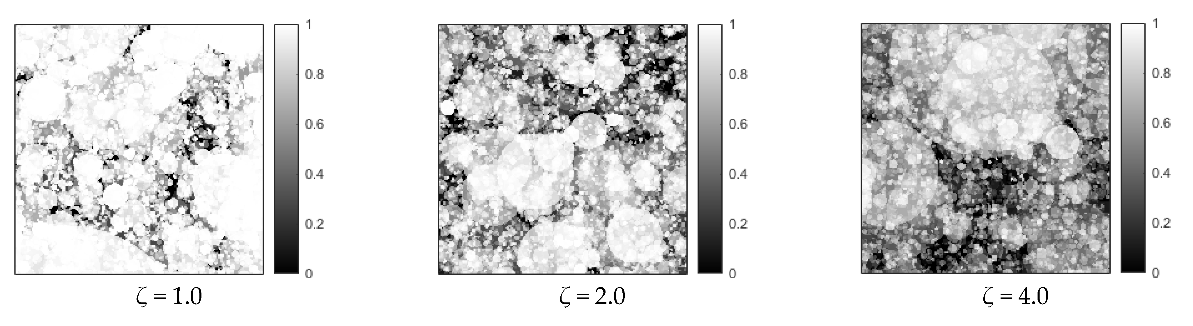
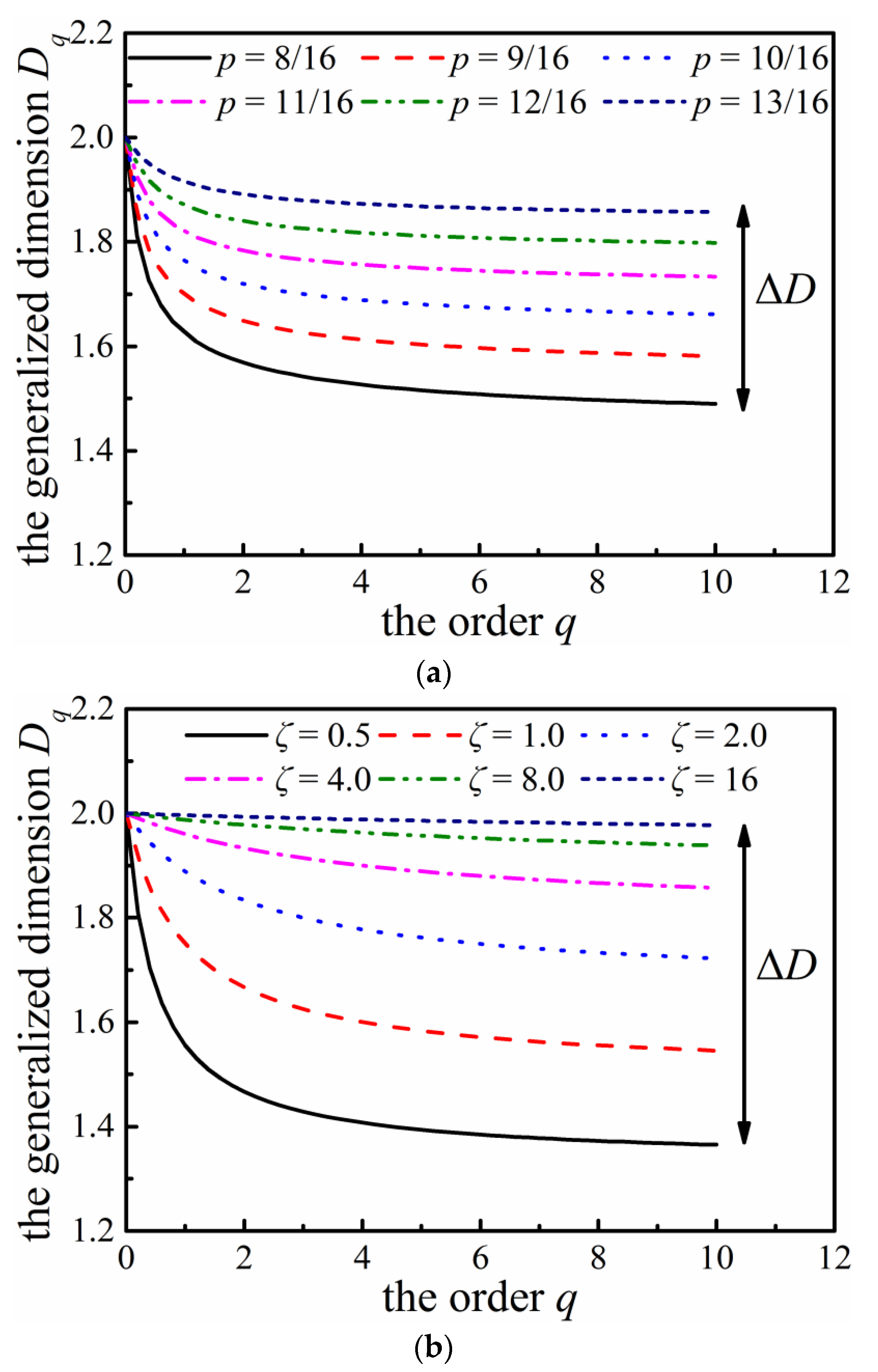
• Two types of cascading algorithms, i.e., two-parameter binomial multiplicative cascades (deterministic) and compound Poisson cascades (stochastic), are employed to synthesize the multifractal fields as well as the porous materials. The range of the Rényi dimension ΔD provides a novel means of quantifying the structural heterogeneity. As the parameter p → 1 (for the two-parameter binomial multiplicative cascades) or ζ >> 1 (for the compound Poisson cascades), one expects to observe rather homogeneous structures.
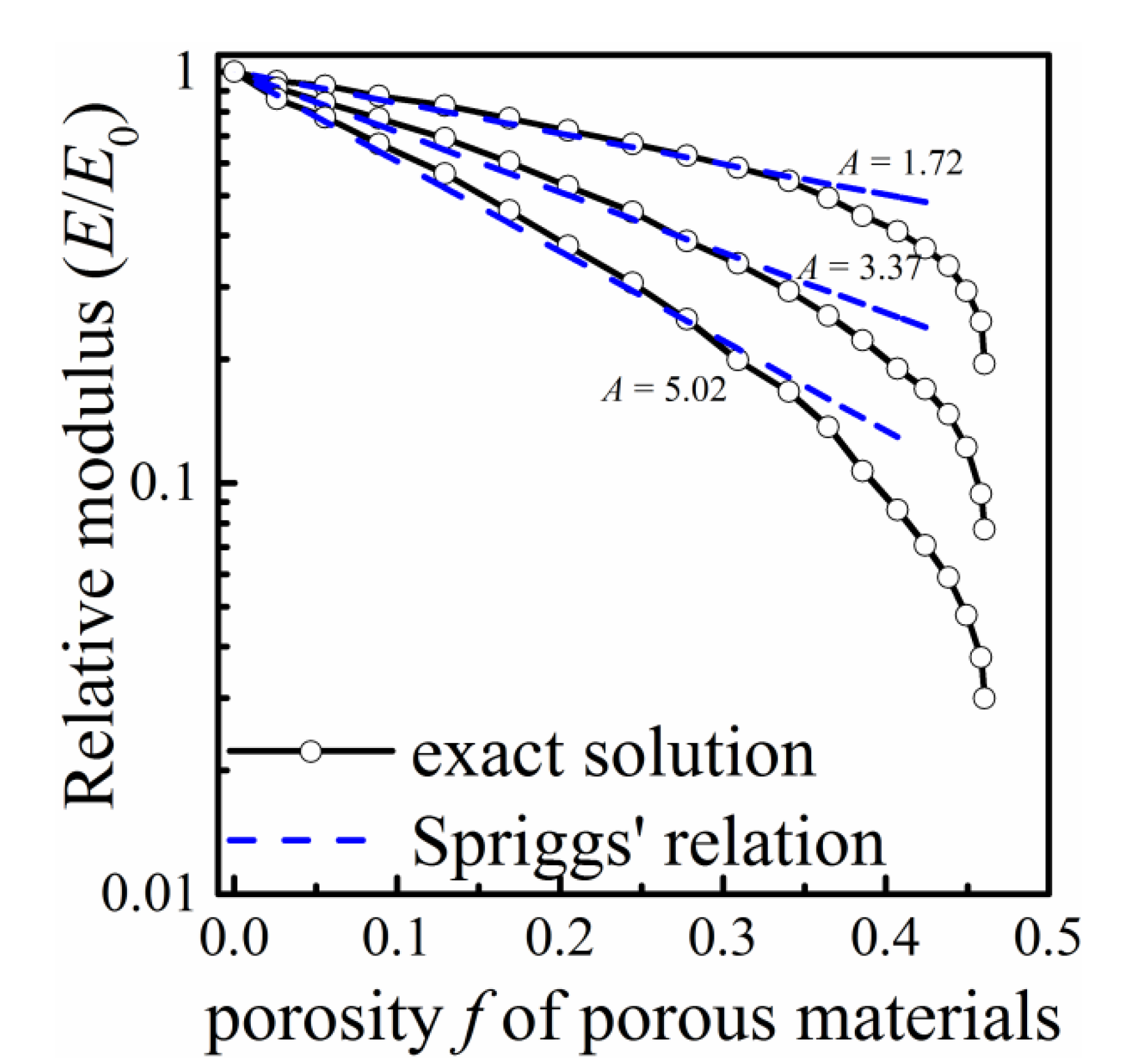
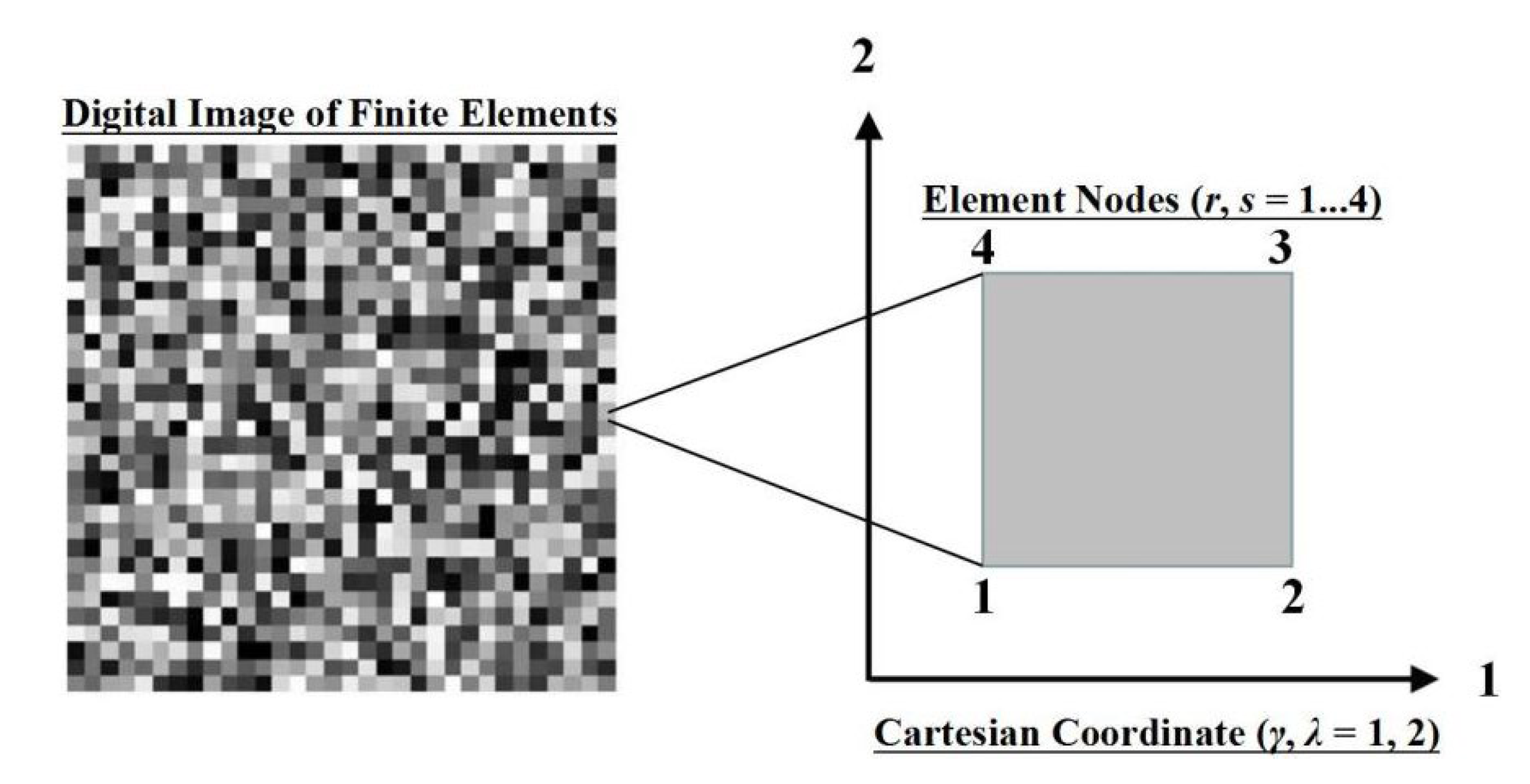
• A mathematical formula, written as E = E₀ exp [–A (g–g_min)/(g_max–g_min)] or E = E₀ exp [–Ag/g_max], is proposed to account for the conversion from the intensity g of a multifractal field to the local elastic modulus E of a multifractal porous material. The finite element method can achieve the homogenization of the local elastic modulus with great efficiency.
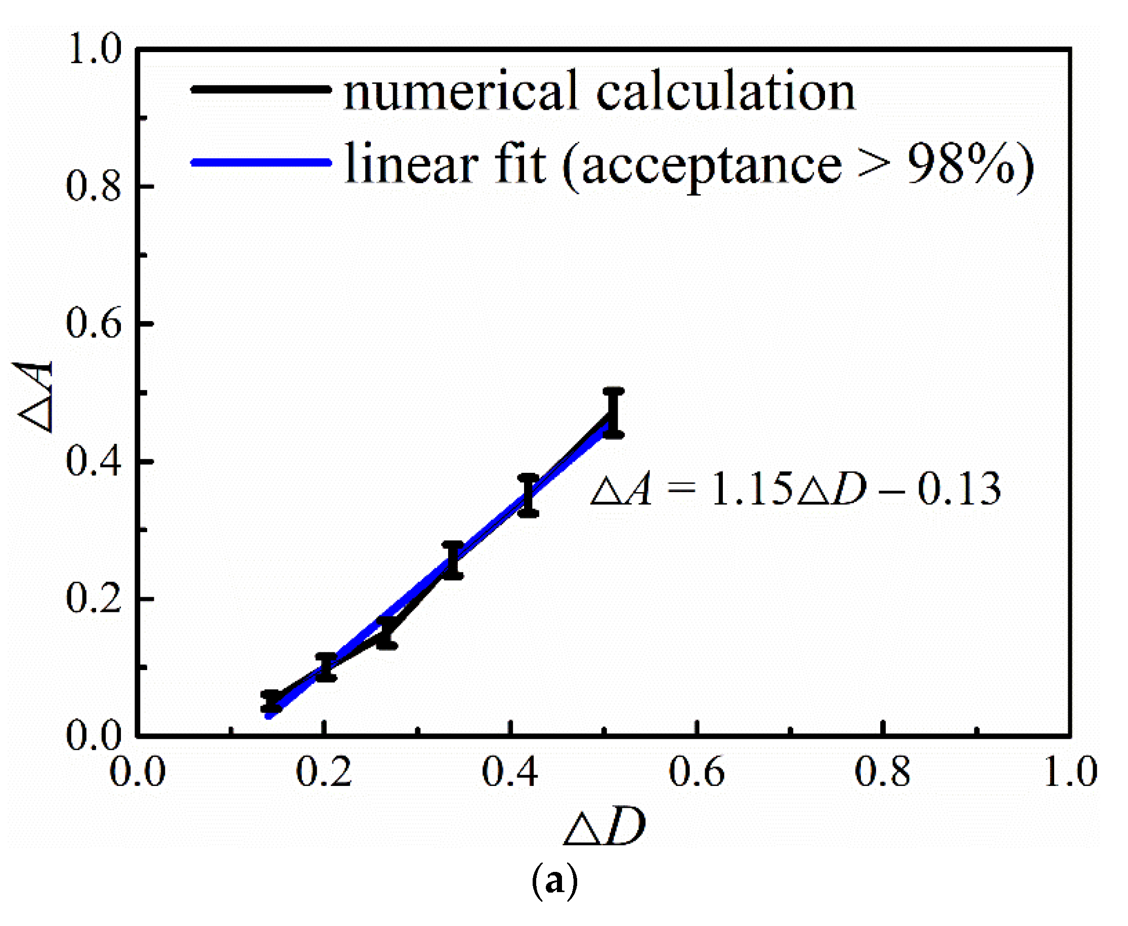
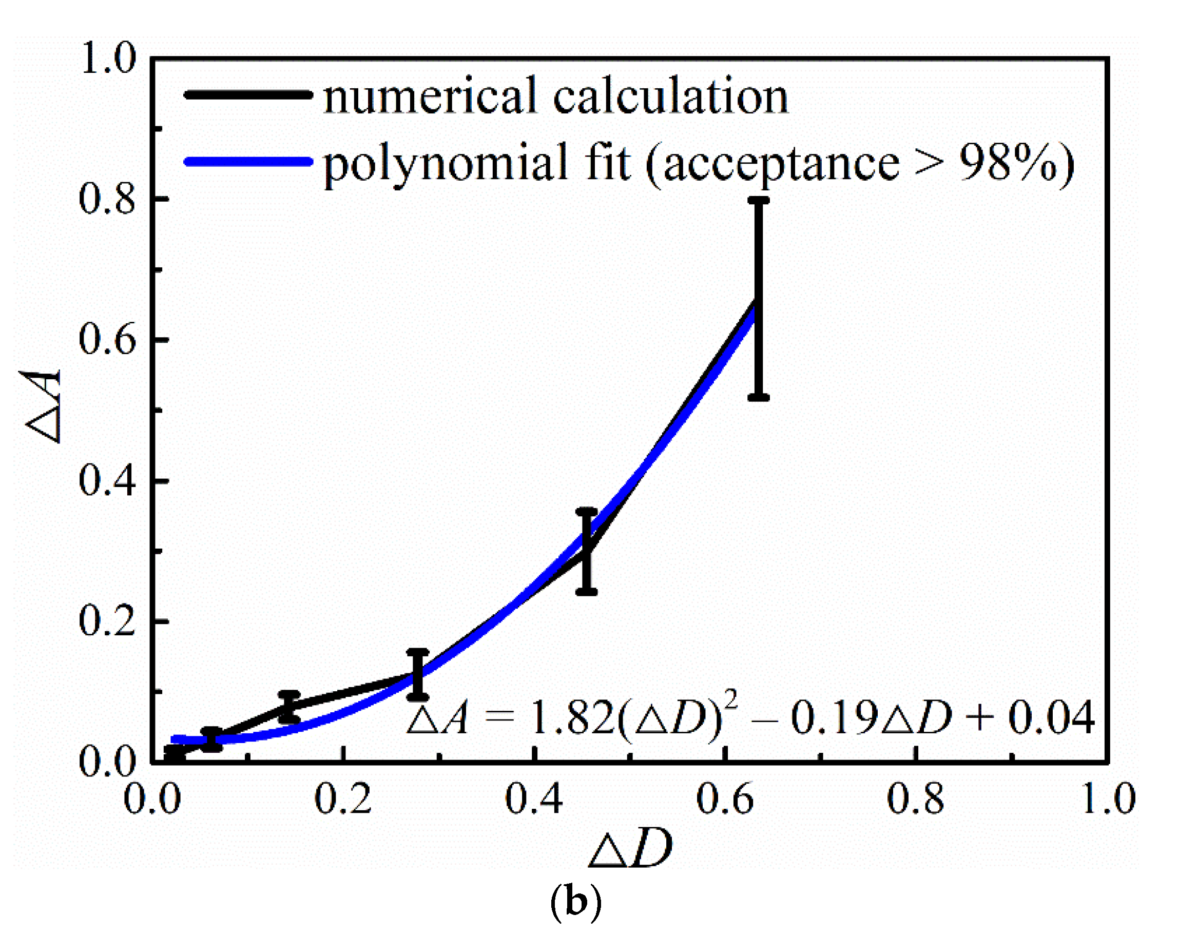
• For the synthesized multifractal porous materials as a whole, the mathematical formula for the macroscopic porosity <f> and the effective elastic modulus E_eff could be described as E_eff = E₀ exp [–(A+ΔA)<f>]. ΔA > 0 is an auxiliary parameter used to quantify the dependence of the effective elastic modulus on the structural heterogeneity. A sound positive correlation exists between ΔA and ΔD, which can be fitted by a linear relation (for the two-parameter binomial multiplicative cascades) or a polynomial relation (for the compound Poisson cascades).

References

1. Chen, C.; Kuang, Y.; Zhu, S.; Burgert, I.; Keplinger, T.; Gong, A.; Li, T.; Berglund, L.; Eichhorn, S.J.; Hu, L.B. Structure–property–function relationships of natural and engineered wood. Nat. Rev. Mater. 2020, 5, 642–666. [Google Scholar] [CrossRef]
2. Roberts, A.P.; Knackstedt, M.A. Structure–property correlations in model composite materials. Phys. Rev. E 1996, 54, 2313–2328. [Google Scholar] [CrossRef] [PubMed] [Green Version]
3. Sun, L.; Marques, M.A.L.; Botti, S. Direct insight into the structure–property relation of interfaces from constrained crystal structure prediction. Nat. Commun. 2021, 12, 811. [Google Scholar] [CrossRef] [PubMed]
4. Poutet, J.; Manzoni, D.; Hage Chehade, F.; Jacquin, C.J.; Bouteca, M.J.; Thovert, J.F.; Adler, P.M. The effective mechanical properties of random porous media. J. Mech. Phys. Solids 1996, 44, 1587–1620. [Google Scholar] [CrossRef]
5. Diamond, S. The microstructure of cement paste and concrete—A visual primer. Cem. Concr. Compos. 2004, 26, 919–933. [Google Scholar] [CrossRef]
6. Allen, A.J.; Thomas, J.J. Analysis of C–S–H gel and cement paste by small–angle neutron scattering. Cem. Concr. Res. 2007, 37, 319–324. [Google Scholar] [CrossRef] [Green Version]
7. Bossa, N.; Chaurand, P.; Vicente, J.; Borschneck, D.; Levard, C.; Aguerre–Chariol, O.; Rose, J. Micro– and nano–X–ray computed–tomography: A step forward in the characterization of the pore network of a leached cement paste. Cem. Concr. Res. 2015, 67, 138–147. [Google Scholar] [CrossRef]
8. Gao, Y.; Wu, K.; Jiang, J.Y. Examination and modeling of fractality for pore–solid structure in cement paste: Starting from the mercury intrusion porosimetry test. Constr. Build. Mater. 2016, 124, 237–243. [Google Scholar] [CrossRef]
9. Kim, J.S.; Chung, S.Y.; Stephan, D.; Han, T.S. Issues on characterization of cement paste microstructures from μ–CT and virtual experiment framework for evaluating mechanical properties. Constr. Build. Mater. 2019, 202, 82–102. [Google Scholar] [CrossRef]
10. Song, Y.; Davy, C.A.; Troadec, D.; Bourbon, X. Pore network of cement hydrates in a high performance concrete by 3D FIB/SEM–implications for macroscopic fluid transport. Cem. Concr. Res. 2019, 115, 308–326. [Google Scholar] [CrossRef]
11. Gao, Y.; Li, W.; Wu, K.; Yuan, Q. Modeling the elastic modulus of cement paste with X–ray computed tomography and a hybrid analytical–numerical algorithm: The effect of structural heterogeneity. Cem. Concr. Compos. 2021, 122, 104145. [Google Scholar] [CrossRef]
12. Shah, H.A.; Yuan, Q.; Zuo, S.H. Air entrainment in fresh concrete and its effects on hardened concrete-a review. Constr. Build. Mater. 2021, 274, 121835. [Google Scholar] [CrossRef]
13. Lopes, R.; Betrouni, N. Fractal and multifractal analysis: A review. Med. Image Anal. 2009, 13, 634–649. [Google Scholar] [CrossRef] [PubMed]
14. San José Martínez, F.; Caniego, F.J.; García Gutiérrez, C.; Espejo, R. Representative elementary area for multifractal analysis of soil porosity using entropy dimension. Nonlin. Process. Geophys. 2007, 14, 503–511. [Google Scholar] [CrossRef]
15. Soto Gómez, D.; Pérez Rodríguez, P.; Vázquez Juíz, L.; Paradelo, M.; Eugenio López Periago, J. 3D multifractal characterization of computed tomography images of soils under different tillage management: Linking multifractal parameters to physical properties. Geoderma 2020, 363, 114129. [Google Scholar] [CrossRef]
16. Guan, M.; Liu, X.P.; Jin, Z.J.; Lai, J. The heterogeneity of pore structure in lacustrine shales: Insights from multifractal analysis using N2 adsorption and mercury intrusion. Mar. Pet. Geol. 2020, 114, 104150. [Google Scholar] [CrossRef]
17. Duan, R.Q.; Xu, Z.F.; Dong, Y.H.; Liu, W.J. Characterization and classification of pore structures in deeply buried carbonate rocks based on mono– and multifractal methods. J. Pet. Sci. Eng. 2021, 203, 108606. [Google Scholar] [CrossRef]
18. Stach, S.; Lamza, A.; Wróbel, Z. 3D image multifractal analysis and pore detection on a stereometric measurement file of a ceramic coating. J. Eur. Ceram. 2014, 34, 3427–3432. [Google Scholar] [CrossRef]
19. Dănilăa, E.; Moraru, L.; Dey, N.; Ashour, A.S.; Shi, F.Q.; Fong, S.J.; Khan, S.; Biswas, A. Multifractal analysis of ceramic pottery SEM images in Cucuteni–Tripolye culture. Optik 2018, 164, 538–546. [Google Scholar] [CrossRef]
20. Valentini, L.; Artioli, G.; Voltolini, M.; Dalconi, M.C. Multifractal analysis of calcium silicate hydrate (C–S–H) mapped by X–ray diffraction microtomography. J. Am. Ceram. Soc. 2012, 95, 2647–2652. [Google Scholar] [CrossRef]
21. Gao, Y.; Gu, Y.H.; Mu, S.; Jiang, J.Y.; Liu, J.P. The multifractal property of heterogeneous microstructure in cement paste. Fractals 2021, 29, 2140006. [Google Scholar] [CrossRef]
22. Bird, N.; Cruz Díaz, M.; Saa, A.; Tarquis, A.m. Fractal and multifractal analysis of pore–scale images of soil. J. Hydrol. 2006, 322, 211–219. [Google Scholar]
23. Mendoza, F.; Verboven, P.; Ho, Q.T.; Kerckhofs, G.; Wevers, M.; Nicolaï, B. Multifractal properties of pore–size distribution in apple tissue using X–ray imaging. J. Food Eng. 2010, 99, 206–215. [Google Scholar] [CrossRef]
24. Arnéodo, A.; Decoster, N.; Roux, S.G. A wavelet–based method for multifractal image analysis. I. Methodology and test applications on isotropic and anisotropic random rough surfaces. Eur. Phys. J. B 2000, 15, 567–600. [Google Scholar] [CrossRef]
25. Decoster, N.; Roux, S.G.; Arnéodo, A. A wavelet–based method for multifractal image analysis. II. Applications to synthetic multifractal rough surfaces. Eur. Phys. J. B 2000, 15, 739–764. [Google Scholar]
26. Saucier, A. Effective permeability of multifractal porous media. Physica A 1992, 183, 381–397. [Google Scholar] [CrossRef]
27. Saucier, A. Scaling of the effective permeability in multifractal porous media. Physica A 1992, 191, 289–294. [Google Scholar] [CrossRef]
28. Perfect, E.; Gentry, R.W.; Sukop, M.C.; Lawson, J.E. Multifractal Sierpinski carpets: Theory and application to upscaling effective saturated hydraulic conductivity. Geoderma 2006, 134, 240–252. [Google Scholar] [CrossRef]
29. Cheng, Q. Generalized binomial multiplicative cascade processes and asymmetrical multifractal distributions. Nonlinear Process. Geophys. 2014, 21, 477–487. [Google Scholar] [CrossRef] [Green Version]
30. Barral, J.; Mandelbrot, B. Multiplicative products of cylindrical pulses. Probab. Theory Relat. Fields 2002, 124, 409–430. [Google Scholar] [CrossRef]
31. Muzy, J.; Bacry, E. Multifractal stationary random measures and multifractal random walks with log–infinitely divisible scaling laws. Phys. Rev. E 2002, 66, 056121. [Google Scholar] [CrossRef] [PubMed] [Green Version]
32. Chainais, P. Multidimensional infinitely divisible cascades. Application to the modelling of intermittency in turbulence. Eur. Phys. J. B 2006, 51, 229–243. [Google Scholar] [CrossRef]
33. Chainais, P. Infinitely divisible cascades to model the statistics of natural Images. IEEE Trans. Pattern Anal. Mach. Intell. 2007, 29, 2105–2119. [Google Scholar] [CrossRef] [PubMed]
34. Hashin, Z.; Shtrikman, S. A variational approach to the theory of the elastic behaviour of multiphase materials. J. Mech. Phys. Solids 1963, 11, 127–140. [Google Scholar] [CrossRef]
35. Budiansky, B.; O'connell, R.J. Elastic moduli of a cracked solid. Int. J. Solids Struct. 1976, 12, 81–97. [Google Scholar]
36. Zhao, Y.H.; Tandon, G.P.; Weng, G.J. Elastic moduli for a class of porous materials. Acta Mech. 1989, 76, 105–130. [Google Scholar] [CrossRef]
37. Gong, S.; Li, Z.; Zhao, Y.Y. An extended Mori–Tanaka model for the elastic moduli of porous materials of finite size. Acta Mater. 2011, 59, 6820–6830. [Google Scholar] [CrossRef]
38. Manoylov, A.V.; Borodich, F.M.; Evans, H.P. Modelling of elastic properties of sintered porous materials. Proc. R. Soc. A 2013, 469, 20120689. [Google Scholar] [CrossRef]
39. Chen, Z.W.; Wang, X.; Giuliani, F.; Atkinson, A. Microstructural characteristics and elastic modulus of porous solids. Acta Mater. 2015, 89, 268–277. [Google Scholar] [CrossRef] [Green Version]
40. Grigorenko, Y.M.; Savula, Y.G.; Mukha, I.S. Linear and nonlinear problems on the elastic deformation of complex shells and methods of their numerical solution. Int. Appl. Mech. 2000, 36, 979–1000. [Google Scholar] [CrossRef]
41. Abbas, I.A.; Zenkour, A. Dual–phase–lag model on thermoelastic interactions in a semi–infinite medium subjected to a ramp-type heating. J. Comput. Theor. Nanosci. 2014, 11, 642–645. [Google Scholar]
42. Abbas, I.A. Eigenvalue approach on fractional order theory of thermoelastic diffusion problem for an infinite elastic medium with a spherical cavity. Appl. Math. Model. 2015, 39, 6196–6206. [Google Scholar]
43. Dyyak, I.I.; Rubino, B.; Savula, Y.H.; Styahar, A.O. Numerical analysis of heterogeneous mathematical model of elastic body with thin inclusion by combined BEM and FEM. Math. Model. Comput. 2019, 6, 239–250. [Google Scholar] [CrossRef]
44. Balankin, A.S. The concept of multifractal elasticity. Phys. Lett. A 1996, 210, 51–59. [Google Scholar]
45. Lashermes, B.; Abry, P.; Chainais, P. New insight in the estimation of scaling exponents. Int. J. Wavelets Multiresolut. Inf. Process. 2004, 2, 497–523. [Google Scholar]
46. Wang, J. Young's modulus of porous materials, Part 1 Theoretical derivation of modulus–porosity correlation. J. Mater. Sci. 1984, 19, 801–808. [Google Scholar]
47. Spriggs, R.M. Expression for effect of porosity on elastic modulus of polycrystalline refractory materials, particularly aluminum oxide. J. Am. Ceram. Soc. 1961, 44, 628–629. [Google Scholar]
48. Kováčik, J. Correlation between Young’s modulus and porosity in porous materials. J. Mater. Sci. Lett. 1999, 18, 1007–1010. [Google Scholar]
49. Roberts, A.P.; Garboczi, E.J. Elastic properties of model porous ceramics. J. Am. Ceram. Soc. 2000, 83, 3041–3048. [Google Scholar]
50. Velez, K.; Maximilien, S.; Damidot, D.; Fantozzi, G.; Sorrentino, F. Determination by nanoindentation of elastic modulus and hardness of pure constituents of Portland cement clinker. Cem. Concr. Res. 2001, 31, 555–561. [Google Scholar]
51. Šmilauer, V.; Bittnar, Z. Microstructure–based micromechanical prediction of elastic properties in hydrating cement paste. Cem. Concr. Res. 2006, 36, 1708–1718. [Google Scholar] [CrossRef]
52. Gao, Y.; Feng, P.; Jiang, J.Y. Analytical and numerical modeling of elastic moduli for cement based composites with solid mass fractal model. Constr. Build. Mater. 2018, 172, 330–339. [Google Scholar] [CrossRef]
53. Wang, J. Young's modulus of porous materials, Part 2 Young's modulus of porous alumina with changing pore structure. J. Mater. Sci. 1984, 19, 809–814. [Google Scholar] [CrossRef]
54. Garboczi, E.J.; Berryman, J.G. Elastic moduli of a material containing composite inclusions: Effective medium theory and finite element computations. Mech. Mater. 2001, 33, 455–470. [Google Scholar] [CrossRef]
55. Huang, J.; Krabbenhoft, K.; Lyamin, A.V. Statistical homogenization of elastic properties of cement paste based on X-ray microtomography images. Int. J. Solids Struct. 2013, 50, 699–709. [Google Scholar] [CrossRef] [Green Version]
56. Meille, S.; Garboczi, E.J. Linear elastic properties of 2–D and 3–D models of porous materials made from elongated objects. Mod. Sim. Mater. Sci. 2001, 9, 371–390. [Google Scholar] [CrossRef]
Figure 1. Schematic of meshing the space of interest in the multifractal analysis of a digital image.
Fractalfract 07 00003 g001
Figure 2. Schematic of the multiplicative cascades for a two-dimensional case.
Fractalfract 07 00003 g002
Figure 3. The multipliers calculated from the truncated binomial distribution of two parameters.
Fractalfract 07 00003 g003
Figure 4. The random multipliers chosen for a particular family of compound Poisson cascades.
Fractalfract 07 00003 g004
Figure 5. Elastic modulus of porous materials, reprinted/adapted with permission from Ref. [46] Wang 1984.
Fractalfract 07 00003 g005
Figure 6. Schematic of the Cartesian coordinates and element nodes for the two-dimensional finite element method.
Fractalfract 07 00003 g006
Figure 7. Multifractal porous materials synthesized by the two-parameter binomial multiplicative cascades.
Fractalfract 07 00003 g007
Figure 8. Multifractal porous materials synthesized by the compound Poisson cascades.
Fractalfract 07 00003 g008
Figure 9. Structural heterogeneity characterized by the range of the Rényi dimension for (a) the two-parameter binomial multiplicative cascades and (b) the compound Pois-son cascades.
Fractalfract 07 00003 g009
Figure 10. Dimensionless strain and stress 1, σ1) within multifractal porous materials synthesized by the two-parameter binomial multiplicative cascades.
Fractalfract 07 00003 g010
Figure 11. Dimensionless strain and stress 1, σ1) within multifractal porous materials synthesized by the compound Poisson cascades.
Fractalfract 07 00003 g011
Figure 12. The variations in ΔA–ΔD for (a) the two-parameter binomial multiplicative cascades and (b) the compound Poisson cascades.
Fractalfract 07 00003 g012aFractalfract 07 00003 g012b