Time-Delay Fractional Variable Order Adaptive Synchronization and Anti-Synchronization between Chen and Lorenz Chaotic Systems Using Fractional Order PID Control

Abstract

In this research work, time-delay adaptive synchronization and adaptive anti-synchronization of chaotic fractional order systems are analyzed via the Caputo fractional derivative, and the prob-lem of synchronization and anti-synchronization of chaotic systems of variable fractional order is solved by using the fractional order PID control law, the adaptive laws of variable-order frac-tional calculus, and a control law deduced from Lyapunov’s theory extended to systems of time-delay variable-order fractional calculus. In this research work, two important problems are solved in the control area: The first problem is described in which deals with syn-chro-nization of chaotic systems of adaptive fractional order with time delay, this problem is solved by using the fractional order PID control law and adaptative laws. The second problem is de-scribed in which deals with anti-synchronization of chaotic systems of adaptive frac-tional order with time delay, and this problem is solved by using the fractional order PID con-trol law and adaptative laws.

1. Introduction

Fractional calculus is currently an area of mathematics widely used to model physical and mechanical systems, information encryption [1], control theory, etc. These are problems that, in his time, Leibnitz did not have to exemplify. The recent theory of differential and integral calculus, developed by Leibnitz and Newton, thus, have answered the question of what would happen if the order of the derivative was a fraction. Currently, we already have enough information about what is known as fractional calculus. In the case of this research, the problem is synchronization and anti-synchronization of chaotic systems described by differential equations of fractional, variable order with estimated adaptable [2] parameters.

To solve the synchronization and anti-synchronization problem, a candidate function of Lyapunov is proposed; this function includes the sum of errors of the states and the parameters of the Lorenz system squared which are parameters that are considered to be unknown, and therefore, they have to be estimated, and for this, adaptation laws are obtained.

The adaptation problem is solved using a candidate Lyapunov function of the form $V=\frac{1}{2}{e}^{T}e+\frac{1}{2}tr\left\{W^{T}W\right\}$, where $e$ is the state vector of the error. In this article, the synchronization and anti-synchronization error $W$ is the weight matrix of the neural network, which is estimated.

As is known: $\frac{1}{2}tr\left\{W^{T}W\right\}=\frac{1}{2}{\displaystyle \sum }_{i,j}^n{W}_{i,j}^2\left(t\right)$, where $W_{i,j}$ are the parameters of the neural network, which are estimated and serve to identify an unknown nonlinear system.

Now, by means of the adaptive laws of chaotic system parameters and a fractional order PID-type control law [3], it is determined that the time derivative of this Lyapunov function is negative definite, and therefore, the problems of synchronization [4] and anti-synchronization [5] are guaranteed.

This research article is organized as follows:

In Section 1, we introduce our research and, in Section 2, we describe the Chen and Lorenz chaotic systems and the variable fractional order PID control law to solve synchronize and anti-synchronize. In Section 3 and Section 4, we obtain the adaptive control laws for synchronization and anti-synchronization and the adaptive laws of variable-order fractional chaotic systems for $\sigma =10, \rho =28, \mathrm{and}\beta =8/3$ variables and present two theorems. In Section 5, we present the simulation results which were favorable with the analytical results, where the errors converge to zero. Finally, in Section 6, we present the conclusions of the results obtained both analytically and via simulation. The results obtained analytically graphically illustrate that adaptive control of the synchronization and anti-synchronization of variable-order fractional chaotic systems is obtained.

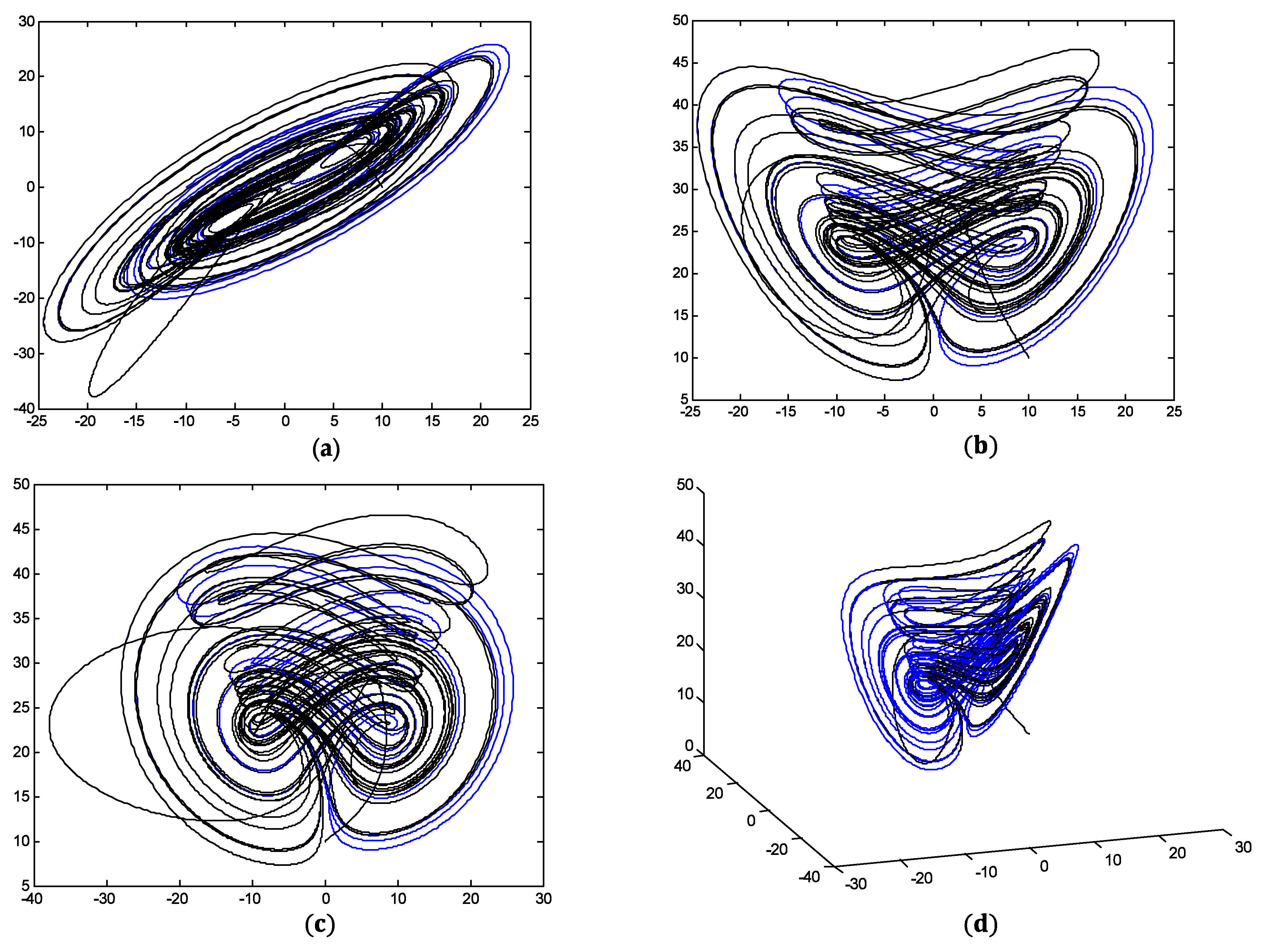
2. Description of the Chen and Lorenz Chaotic Systems

In this section, the variable-order fractional chaotic systems are proposed that are considered in this work, namely the master system, i.e., the Chen system, and the slave system, i.e., the Lorenz system.

For the systems to synchronize and anti-synchronize, in this research work, we use variable-order fractional calculus in the sense of Caputo [6,7,8] as described below.

First, we present the Chen chaotic system which we call the master system.

The Chen system is given by [9]:

$$\begin{array}{l}\frac{d^{{\alpha }_1}x}{d{t}^{{\alpha }_1}}=35y-35x,\\ \frac{d^{{\alpha }_2}y}{d{t}^{{\alpha }_2}}=-7x-xz+28y\\ \frac{d^{{\alpha }_3}z}{d{t}^{{\alpha }_3}}=xy-3z,\end{array}$$

(1)

with initial conditions ${\left(-10, 0,37\right)}^T.$

Now, we present the Lorenz system, which we call the slave system:

The Lorenz system is given by [10]:

$$\begin{array}{l}\frac{d^{{\alpha }_1}{x}_1}{d{t}^{{\alpha }_1}}=10x_2-10x_1,\\ \frac{d^{{\alpha }_2}{x}_2}{d{t}^{{\alpha }_2}}=-x_2-x_1{x}_2+28x_1,\\ \frac{d^{{\alpha }_3}{x}_3}{d{t}^{{\alpha }_3}}=x_1{x}_2-\left(\frac{8}{3}\right)x_3,\end{array}$$

(2)

with initial conditions ${\left(10, 0, 10\right)}^T.$

To solve the synchronization and anti-synchronization problem, we use the following fractional order PID control [11]:

$$PI{D}_j=u\left(t\right)=K_{p_j}{e}_j\left(t\right)+K_{i_j}{D}_t^{-\lambda }{e}_j\left(t\right)+K_{d_j}{D}_t^{\mu }{e}_j\left(t\right),j=1,2,3$$

where $K_p$, $K_i$, $K_d\in ℝ$, and $\lambda$, $\mu {ℝ}^{+}$ are the parameters; $\lambda , \mu$ are the orders of the derivative with $\lambda , \mu \in \left(0,1\right]$.

In the next section, the synchronization problem is solved, which are usually used to control systems, in this case synchronizing and anti-synchronizing chaotic systems, where λ, μ are the orders of the derivative in which λ, μ ∈(0,1] is often used.

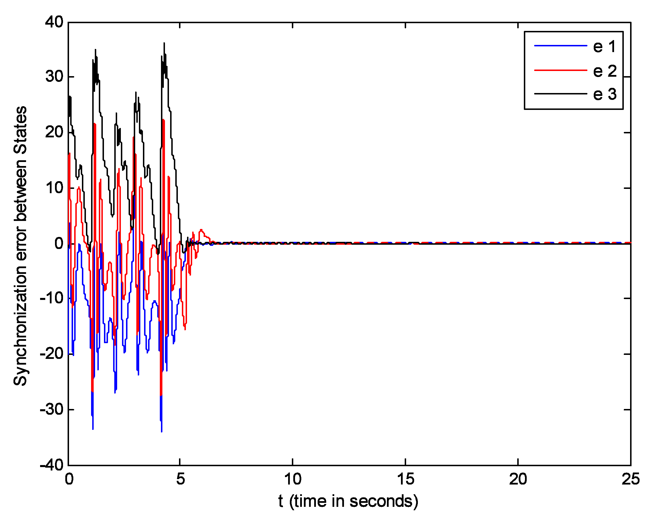
3. Time-Delay Adaptive Synchronization of Chaotic Systems of Fractional Order

In this synchronization section, the chaotic system described by (2) is forced to synchronize with system (1), for which, as usual in control systems, we include a control (adaptive control laws). To achieve this objective, the control laws are: $u_i+PI{D}_i, i=1, 2, \mathrm{and} 3$, and since we are working with adaptive synchronization, we consider σ, ρ, and β to be the unknown parameters of the control system described by (4).

Let (4) be the control system which will be forced to synchronize with system (3). Then, the Chen system is:

$$\begin{array}{l}\frac{d^{{\alpha }_2}y}{d{t}^{{\alpha }_2}}=\left(c-a\right)x-xz+cy,\\ \frac{d^{{\alpha }_3}z}{d{t}^{{\alpha }_3}}=xy-bz,\end{array}$$

(3)

where $a=35,b=3,\mathrm{and}c=28$, with ${\left(-10,0,37\right)}^T$.

The time-delay Lorenz system is given by:

$$\begin{array}{l}{\dot{x}}_1=\frac{d^{\alpha }{x}_1}{d{t}^{\alpha }}=\sigma \left(x_2\left(t-\tau \right)-x_1\right)+u_1+PI{D}_1,\\ {\dot{x}}_2=\frac{d^{\alpha }{x}_2}{d{t}^{\alpha }}=\rho x_1\left(t-\tau \right)-x_1{x}_2-x_2+u_2+PI{D}_2,\\ {\dot{x}}_3=\frac{d^{\alpha }{x}_3}{d{t}^{\alpha }}=-\beta x_3\left(t-\tau \right)+x_1{x}_2+u_3+PI{D}_3,\end{array}$$

(4)

where $\sigma , \rho , \mathrm{and}\beta$ are unknown, with ${\left(10,0,10\right)}^T.$

Let the errors of the Chen-Lorenz states be [12]:

$$e_1=x_1-x,e_2=x_2-y,e_3=x_3-z,$$

(5)

and the dynamics of the errors are [13]:

$$\begin{array}{l}\frac{d^{\alpha }{e}_1}{d{t}^{\alpha }}=\frac{d^{\alpha }{x}_1}{d{t}^{\alpha }}-\frac{d^{\alpha }\mathrm{x}}{d{t}^{\alpha }}=\sigma \left(x_2\left(t-\tau \right)-x_1\right)+u_1-a\left(y-x\right)+PI{D}_1,\\ \frac{d^{\alpha }{e}_2}{d{t}^{\alpha }}=\frac{d^{\alpha }{x}_2}{d{t}^{\alpha }}-\frac{d^{\alpha }\mathrm{y}}{d{t}^{\alpha }}=\rho x_1\left(t-\tau \right)-x_1{x}_2-x_2+u_2-\left(c-a\right)x+xz-cy+PI{D}_2,\\ \frac{d^{\alpha }{e}_3}{d{t}^{\alpha }}=\frac{d^{\alpha }{x}_3}{d{t}^{\alpha }}-\frac{d^{\alpha }\mathrm{z}}{d{t}^{\alpha }}=-\beta x_3\left(t-\tau \right)+x_1{x}_2+u_3-xy+bz+PI{D}_3,\end{array}$$

(6)

To guarantee that the dynamics of the errors converge to zero, which implies that the time-delay systems synchronize and anti-synchronize, we use the following candidate Lyapunov function, which depends on the errors of the states and the adaptive parameters of the system. Note, we have already used this Lyapunov function extensively in previous works written by the authors of this article [14].

We select the following Lyapunov function [15]:

$$V=\frac{1}{2}\left(e_1^2+e_2^2+e_3^2\right)+\frac{1}{2}\left({\tilde{\sigma }}^2+{\tilde{\rho }}^2+{\tilde{\beta }}^2\right),$$

(7)

where $\frac{d^{\alpha }V}{d{t}^{\alpha }}\triangleq \frac{d^{\alpha }{V}_1}{d{t}^{\alpha }}+\frac{d^{\alpha }{V}_2}{d{t}^{\alpha }}+\frac{d^{\alpha }{V}_3}{d{t}^{\alpha }}$,

$$\frac{d^{\alpha }V}{d{t}^{\alpha }}=e_1\frac{d^{\alpha }{e}_1}{d{t}^{\alpha }}+e_2\frac{d^{\alpha }{e}_2}{d{t}^{\alpha }}+e_3\frac{d^{\alpha }{e}_3}{d{t}^{\alpha }}+\tilde{\sigma }\frac{d^{\alpha }\tilde{\sigma }}{d{t}^{\alpha }}+\tilde{\rho }\frac{d^{\alpha }\tilde{\rho }}{d{t}^{\alpha }}+\tilde{\beta }\frac{d^{\alpha }\tilde{\beta }}{d{t}^{\alpha }}.$$

(8)

Let us define:

$$\begin{array}{ll}\frac{d^{\alpha }{V}_1}{d{t}^{\alpha }}& =e_1\frac{d^{\alpha }{e}_1}{d{t}^{\alpha }}=e_1\left[\sigma \left(x_2\left(t-\tau \right)-x_1\right)+u_1-a\left(y-x\right)+PID\right],\\ & =e_1\left[\sigma \left(x_2\left(t-\tau \right)-x_1\right)+u_1-a\left(y-x\right)+PID\right],\end{array}$$

(9)

Adding and subtracting $\overline{\sigma }\left(x_2\left(t-\tau \right)-x_1\right),e_1$, we have already used this methodology of adding and subtracting terms in previous articles [16]:

$$\frac{d^{\alpha }{V}_1}{d{t}^{\alpha }}=e_1\left[\left(\sigma -\overline{\sigma }\right)\left(x_2\left(t-\tau \right)-x_1\right)+u_1-a\left(y-x\right)+\overline{\sigma }\left(x_2\left(t-\tau \right)-x_1\right)+e_1-e_1+PI{D}_1\right].$$

We select

$$\tilde{\sigma }=\left(\sigma -\overline{\sigma }\right),$$

(10)

where we obtain:

$$\frac{d^{\alpha }\tilde{\sigma }}{d{t}^{\alpha }}=-\frac{d^{\alpha }\overline{\sigma }}{d{t}^{\alpha }},$$

(11)

as $\frac{d^{\alpha }\sigma }{d{t}^{\alpha }}=0$, since $\sigma$ it is a constant [17].

From $\frac{d^{\alpha }{V}_1}{d{t}^{\alpha }}$, we select the control action:

$$u_1=a\left(y-x\right)-\overline{\sigma }\left(x_2\left(t-\tau \right)-x_1\right)-e_1-PI{D}_1,$$

(12)

so that:

$$\frac{d^{\alpha }{V}_1}{d{t}^{\alpha }}=e_1\tilde{\sigma }\left(x_2\left(t-\tau \right)-x_1\right)-e_1^2.$$

(13)

Similarly, now,$\frac{d^{\alpha }{V}_2}{d{t}^{\alpha }}$ is:

$$\frac{d^{\alpha }{V}_2}{d{t}^{\alpha }}=e_2\frac{d^{\alpha }{e}_2}{d{t}^{\alpha }}=e_2\left[\rho x_1\left(t-\tau \right)-x_1{x}_2-x_2+u_2-\left(c-a\right)x+xz-cy+PI{D}_2\right].$$

(14)

Adding and subtracting $\overline{\rho }{x}_1\left(t-\tau \right),e_2:$

$$\begin{gathered} \frac{d^{\alpha }{V}_2}{d{t}^{\alpha }}=e_2[\left(\rho -\overline{\rho }\right)x_1\left(t-\tau \right)-x_1{x}_2-x_2+u_2-\left(c-a\right)x+xz-cy+ \\ \overline{\rho }{x}_1\left(t-\tau \right)+e_2-e_2+PI{D}_2. \end{gathered}$$

Here,

$$\tilde{\rho }=\left(\rho -\overline{\rho }\right),$$

(15)

$$\frac{d^{\alpha }\tilde{\rho }}{d{t}^{\alpha }}=-\frac{d^{\alpha }\overline{\rho }}{d{t}^{\alpha }},$$

(16)

since $\rho$ it is a constant, as $\frac{d^{\alpha }\rho }{d{t}^{\alpha }}=0$, and the control action is:

$$u_2=x_1{x}_2+x_2+\left(c-a\right)x-xz+cy-\overline{\rho }{x}_1\left(t-\tau \right)-e_2-PI{D}_2,$$

(17)

$$\frac{d^{\alpha }{V}_2}{d{t}^{\alpha }}=e_2\tilde{\rho }{x}_1\left(t-\tau \right)-e_2^2$$

(18)

$$\frac{d^{\alpha }{V}_3}{d{t}^{\alpha }}=e_3\frac{d^{\alpha }{e}_3}{d{t}^{\alpha }}=e_3\left[-\beta x_3\left(t-\tau \right)+x_1{x}_2+u_3-xy+bz+PI{D}_3\right],$$

(19)

and, $\frac{d^{\alpha }{V}_3}{d{t}^{\alpha }}$ is, adding and subtracting $\overline{\beta }{x}_3\left(t-\tau \right), e_3$,

$$\frac{d^{\alpha }{V}_3}{d{t}^{\alpha }}=e_3\left[-\left(\beta -\overline{\beta }\right)x_3\left(t-\tau \right)+x_1{x}_2+u_3+bz-xy-\overline{\beta }{x}_3\left(t-\tau \right)+e_3-e_3+PI{D}_3\right].$$

Here,

$$\tilde{\beta }=\left(\beta -\overline{\beta }\right),$$

(20)

$$\frac{d^{\alpha }\tilde{\beta }}{d{t}^{\alpha }}=-\frac{d^{\alpha }\overline{\beta }}{d{t}^{\alpha }},$$

(21)

as $\frac{d^{\alpha }\beta }{d{t}^{\alpha }}=0$, since$\beta$ it is a constant.

Finally we obtain the control law $u_3$:

$$u_3=-x_1{x}_2-bz+xy+\overline{\beta }{x}_3\left(t-\tau \right)-e_3-PI{D}_3,$$

(22)

$$\frac{d^{\alpha }{V}_3}{d{t}^{\alpha }}=-e_{3 }\tilde{\beta }{x}_3\left(t-\tau \right)-e_3^2.$$

(23)

In summary we have:

$$\begin{gathered} \frac{d^{\alpha }V}{d{t}^{\alpha }}=\frac{d^{\alpha }{V}_1}{d{t}^{\alpha }}+\frac{d^{\alpha }{V}_2}{d{t}^{\alpha }}+\frac{d^{\alpha }{V}_3}{d{t}^{\alpha }}, \\ \frac{d^{\alpha }V}{d{t}^{\alpha }}=e_1\tilde{\sigma }\left(x_2\left(t-\tau \right)-x_1\right)-e_1^2+e_2\tilde{\rho }{x}_1\left(t-\tau \right)-e_2^2-e_3\tilde{\beta }{x}_3\left(t-\tau \right)- \\ {e}_3^2+\tilde{\sigma }\frac{d^{\alpha }\tilde{\sigma }}{d{t}^{\alpha }}+\tilde{\rho }\frac{d^{\alpha }\tilde{\rho }}{d{t}^{\alpha }}+\tilde{\beta }\frac{d^{\alpha }\tilde{\beta }}{d{t}^{\alpha }}. \end{gathered}$$

(24)

From (11), (16), and (21), we select the following adaptation law for $\tilde{\sigma }, \tilde{\rho }$, and $\tilde{\beta }$, and we have, $\frac{d^{\alpha }\tilde{\sigma }}{d{t}^{\alpha }}=-\frac{d^{\alpha }\overline{\sigma }}{d{t}^{\alpha }}$, $e_1\tilde{\sigma }\left(x_2\left(t-\tau \right)-x_1\right)+\tilde{\sigma }\frac{d^{\alpha }\tilde{\sigma }}{d{t}^{\alpha }}=0$, where $\tilde{\sigma }\ne 0$, then

$$\frac{d^{\alpha }\overline{\sigma }}{d{t}^{\alpha }}=e_1\left(x_2\left(t-\tau \right)-x_1\right).$$

(25)

Now, in (16), $\frac{d^{\alpha }\tilde{\rho }}{d{t}^{\alpha }}=-\frac{d^{\alpha }\overline{\rho }}{d{t}^{\alpha }}$, $e_2\tilde{\rho }{x}_1\left(t-\tau \right)+\tilde{\rho }\frac{d^{\alpha }\tilde{\rho }}{d{t}^{\alpha }}=0$, and $\tilde{\rho }\ne 0$, we have

$$\frac{d^{\alpha }\overline{\rho }}{d{t}^{\alpha }}=e_2{x}_1\left(t-\tau \right).$$

(26)

Finally, in (21), $\frac{d^{\alpha }\tilde{\beta }}{d{t}^{\alpha }}=-\frac{d^{\alpha }\overline{\beta }}{d{t}^{\alpha }}$,

$$\begin{gathered} -e_3\tilde{\beta }{x}_3\left(t-\tau \right)+\tilde{\beta }\frac{d^{\alpha }\tilde{\beta }}{d{t}^{\alpha }}=0,\tilde{\beta }\ne 0, \\ \frac{d^{\alpha }\overline{\beta }}{d{t}^{\alpha }}=-e_3{x}_3\left(t-\tau \right). \end{gathered}$$

(27)

With the above you have: $\frac{d^{\alpha }V}{d{t}^{\alpha }}=-e_1^2-e_2^2-e_3^2<0,\forall e_1,e_2,e_3,$and

$$\therefore \underset{t\to \infty }{\lim }e\left(t\right)=0$$

with which, the time-delay system (4) is synchronized with system (3), using the control laws obtained previously (12), (17), and (22) and the adaptation laws (estimation), given by Equations (25)–(27). Therefore, we have the following theorem:

Theorem 1. 

The slave system described by the Lorenz differential Equation (2) is adaptively synchronized with the master system, i.e., the Chen chaotic system (1), using the laws of adaptation, the the fractional order PID-type control law and a control law derived from a candidate Lyapunov function for systems of variable fractional order.

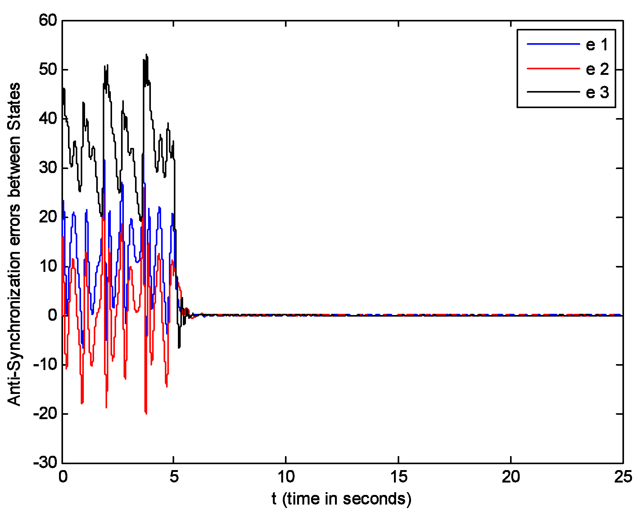
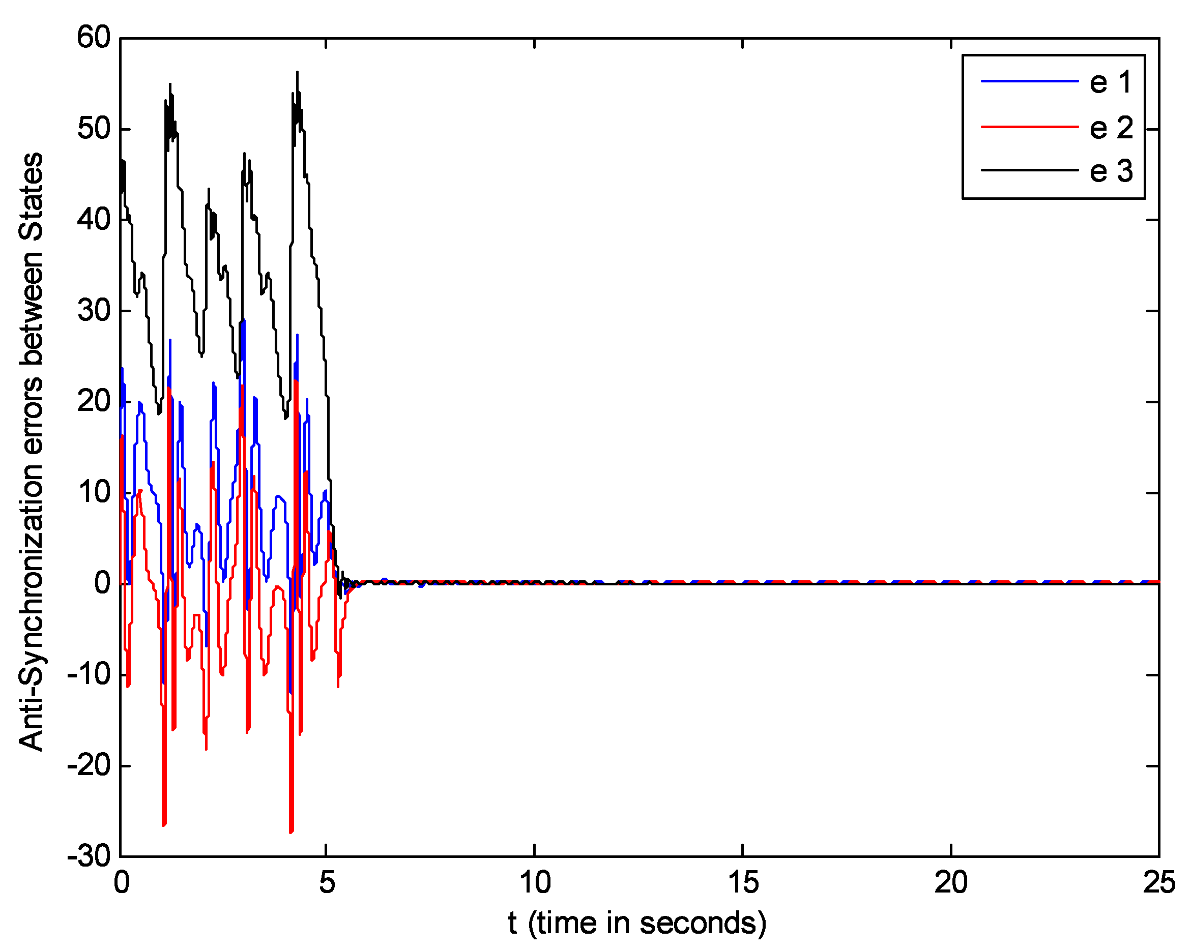
4. Time-Delay Adaptive Anti-Synchronization of Fractional Order Chaotic Systems

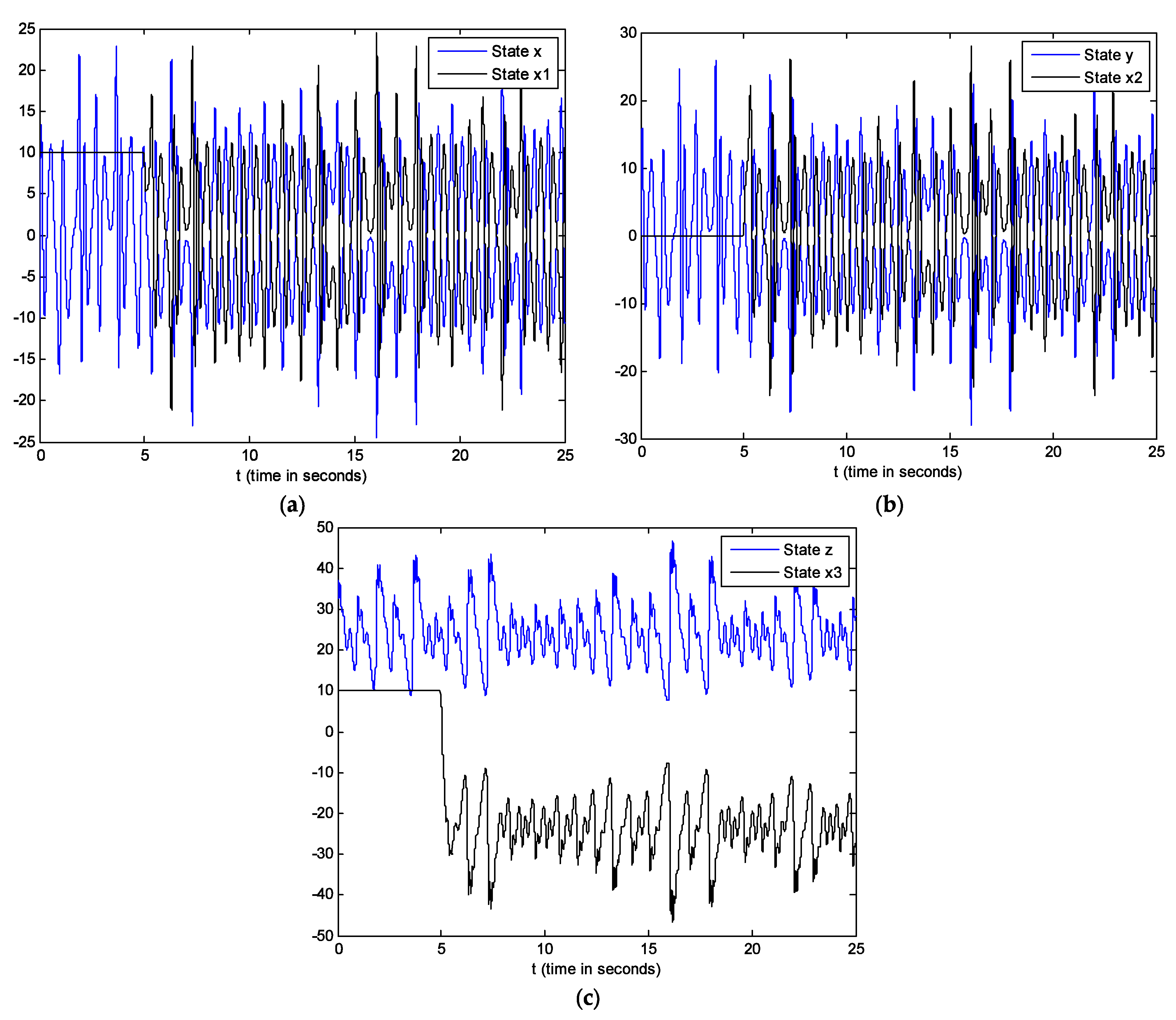
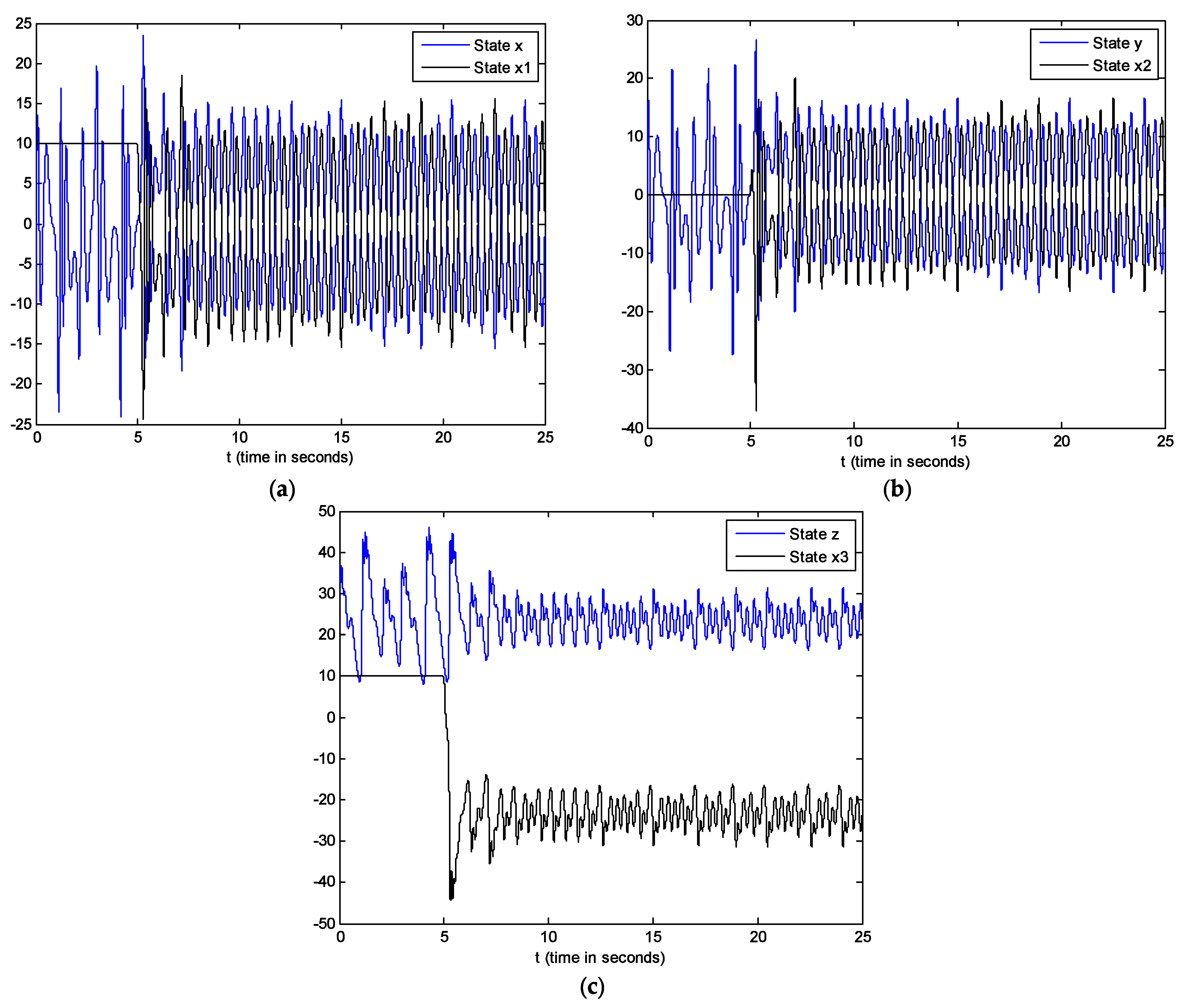
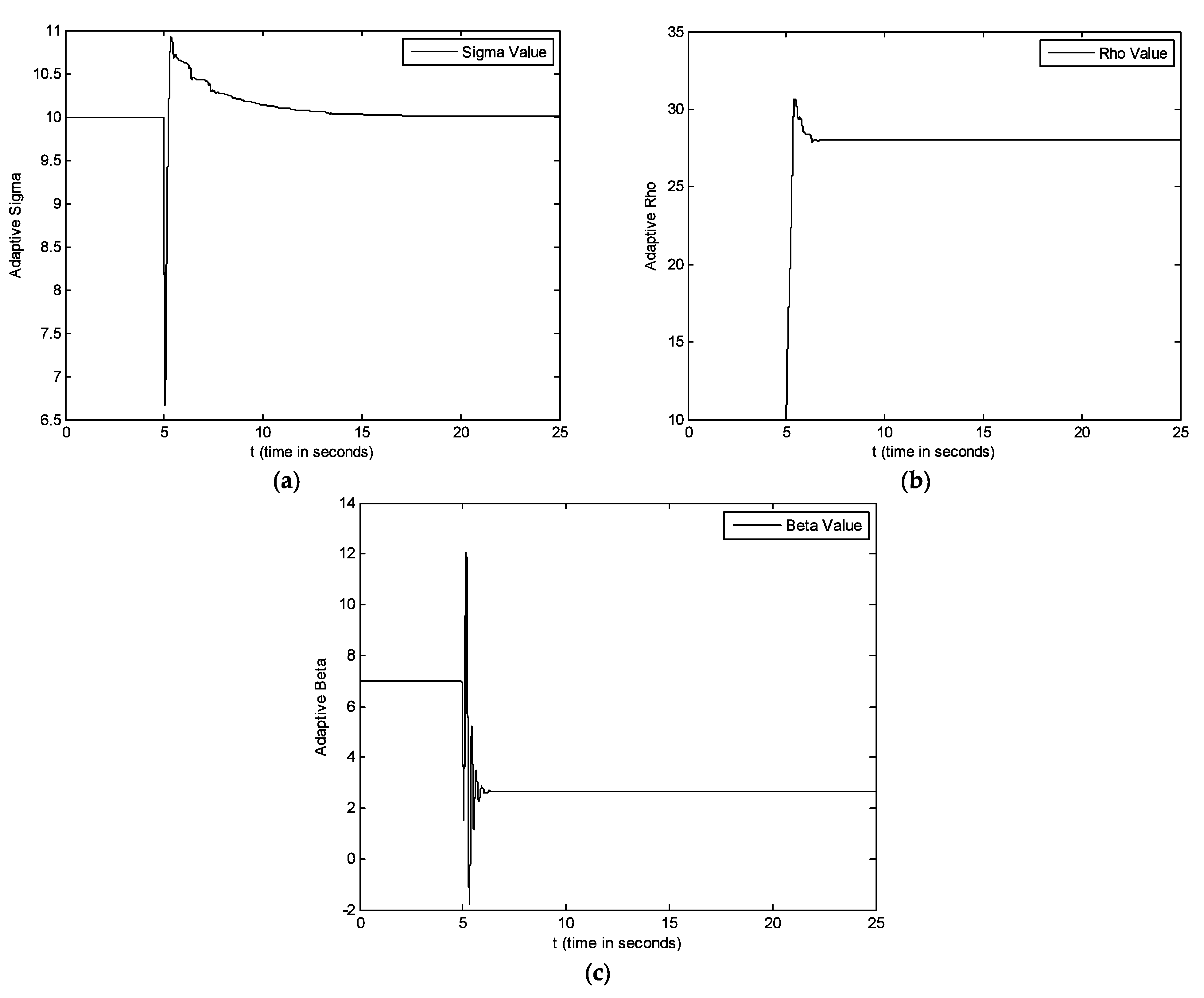
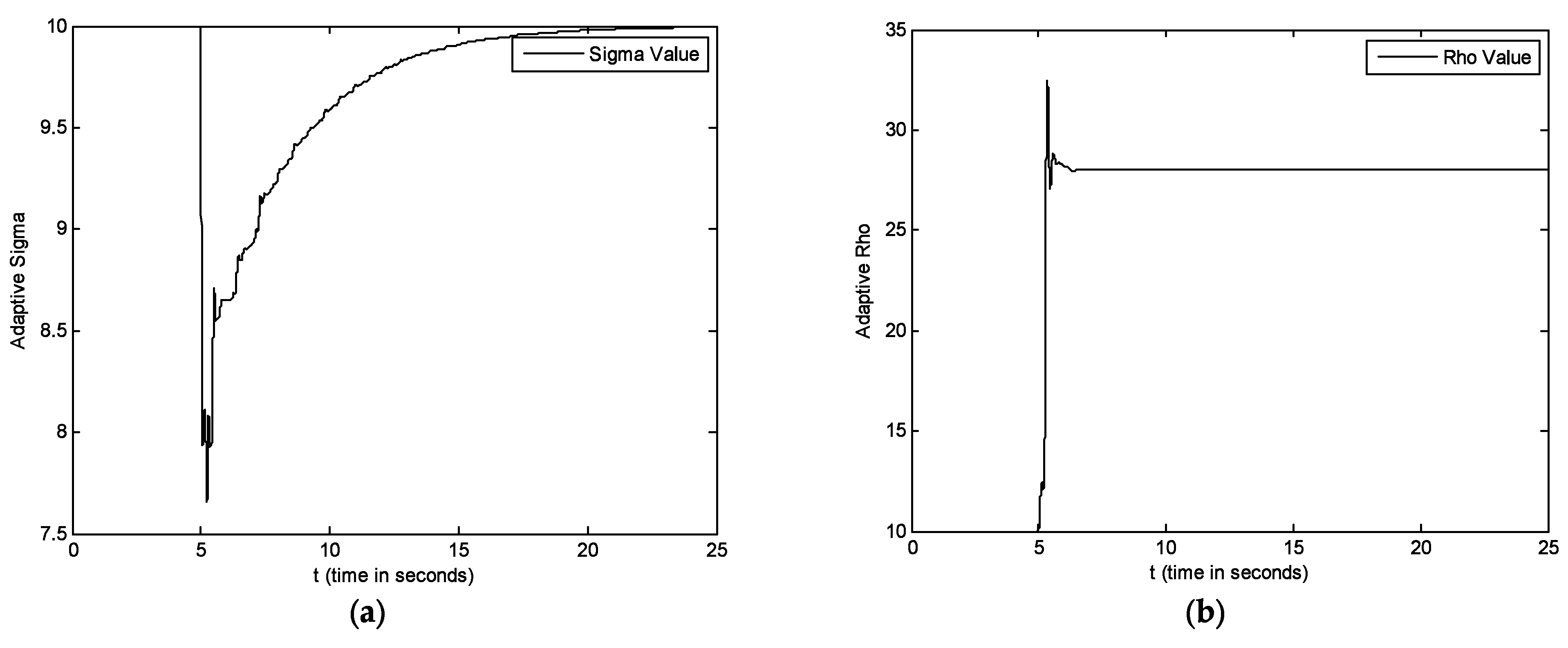
In this anti-synchronization section, the chaotic system described by (2) is forced to anti-synchronize with system (1), for which, as usual in control systems, we include a control (adaptive control laws). To achieve this objective, the control laws are: $u_i+PI{D}_i, i=1, 2, \mathrm{and}3$, and since we are working with adaptive anti-synchronization we consider σ, ρ, and β to be the unknown parameters of the control system described by (4). In this section, we solve the anti-synchronization problem between two chaotic systems, the master Chen system and the slave Lorenz system, where we consider that the systems have a time delay $\tau \in {ℝ}^{+}$. Let the time-delay Lorenz system (4) be a control system which will be forced to the anti-synchronize with the Chen system (3).

Let the errors of the Chen-Lorenz states be [12]

Below, we express the errors in the states of these systems, which are given by:

$$e_1=x_1+x,e_2=x_2+y,e_3=x_3+z,$$

(28)

and the dynamics of the errors are:

$$\begin{array}{l}\frac{d^{\alpha }{e}_1}{d{t}^{\alpha }}=\frac{d^{\alpha }{x}_1}{d{t}^{\alpha }}+\frac{d^{\alpha }\mathrm{x}}{d{t}^{\alpha }}=\sigma \left(x_2\left(t-\tau \right)-x_1\right)+u_1+a\left(y-x\right)+PI{D}_1,\\ \frac{d^{\alpha }{e}_2}{d{t}^{\alpha }}=\frac{d^{\alpha }{x}_2}{d{t}^{\alpha }}+\frac{d^{\alpha }\mathrm{y}}{d{t}^{\alpha }}=\rho x_1\left(t-\tau \right)-x_1{x}_2-x_2+u_2+\left(c-a\right)x-xz+cy+PI{D}_2,\\ \frac{d^{\alpha }{e}_3}{d{t}^{\alpha }}=\frac{d^{\alpha }{x}_3}{d{t}^{\alpha }}+\frac{d^{\alpha }\mathrm{z}}{d{t}^{\alpha }}=-\beta x_3\left(t-\tau \right)+x_1{x}_2+u_3+xy-bz+PI{D}_3.\end{array}$$

(29)

We select the following Lyapunov function [15]:

$$V=\frac{1}{2}\left(e_1^2+e_2^2+e_3^2\right)+\frac{1}{2}\left({\tilde{\sigma }}^2+{\tilde{\rho }}^2+{\tilde{\beta }}^2\right),$$

(30)

and as is known, we obtain the derivative of V along the trajectories of (29). These are given by (31), and we do this also in the synchronization:

$$\frac{d^{\alpha }V}{d{t}^{\alpha }}=e_1\frac{d^{\alpha }{e}_1}{d{t}^{\alpha }}+e_2\frac{d^{\alpha }{e}_2}{d{t}^{\alpha }}+e_3\frac{d^{\alpha }{e}_3}{d{t}^{\alpha }}+\tilde{\sigma }\frac{d^{\alpha }\tilde{\sigma }}{d{t}^{\alpha }}+\tilde{\rho }\frac{d^{\alpha }\tilde{\rho }}{d{t}^{\alpha }}+\tilde{\beta }\frac{d^{\alpha }\tilde{\beta }}{d{t}^{\alpha }},$$

(31)

$$\frac{d^{\alpha }{V}_1}{d{t}^{\alpha }}=e_1\frac{d^{\alpha }{e}_1}{d{t}^{\alpha }}=e_1\left[\sigma \left(x_2\left(t-\tau \right)-x_1\right)+u_1-a\left(y-x\right)+PI{D}_1\right].$$

(32)

Adding and subtracting $\overline{\sigma }\left(x_2\left(t-\tau \right)-x_1\right),e_1$,

$$\frac{d^{\alpha }{V}_1}{d{t}^{\alpha }}=e_1\left[\left(\sigma -\overline{\sigma }\right)\left(x_2\left(t-\tau \right)-x_1\right)+u_1+a\left(y-x\right)+\overline{\sigma }\left(x_2\left(t-\tau \right)-x_1\right)+e_1-e_1+PI{D}_1\right].$$

We select:

$$\tilde{\sigma }=\left(\sigma -\overline{\sigma }\right),$$

(33)

$$\frac{d^{\alpha }\tilde{\sigma }}{d{t}^{\alpha }}=-\frac{d^{\alpha }\overline{\sigma }}{d{t}^{\alpha }},$$

(34)

where$\sigma$ is zero since it is a constant.

The control action is:

$$u_1=-a\left(y-x\right)-\overline{\sigma }\left(x_2\left(t-\tau \right)-x_1\right)-e_1-PI{D}_1,$$

(35)

$$\frac{d^{\alpha }{V}_1}{d{t}^{\alpha }}=e_1\tilde{\sigma }\left(x_2\left(t-\tau \right)-x_1\right)-e_1^2.$$

(36)

Now,$\frac{d^{\alpha }{V}_2}{d{t}^{\alpha }}$ is

$$\frac{d^{\alpha }{V}_2}{d{t}^{\alpha }}=e_2\frac{d^{\alpha }{e}_2}{d{t}^{\alpha }}=e_2\left[\rho x_1\left(t-\tau \right)-x_1{x}_2-x_2+u_2+\left(c-a\right)x-xz+cy+PI{D}_2\right].$$

(37)

Adding and subtracting $\overline{\rho }{x}_1, e_2$:

$$\begin{gathered} \frac{d^{\alpha }{V}_2}{d{t}^{\alpha }}=e_2\left[\left(\rho -\overline{\rho }\right)x_1\left(t-\tau \right)-x_1{x}_2-x_2+u_2+\left(c-a\right)x-xz+cy \\ +\overline{\rho }{x}_1\left(t-\tau \right)+e_2-e_2+PI{D}_2\right]. \end{gathered}$$

Here,

$$\tilde{\rho }=\left(\rho -\overline{\rho }\right),$$

(38)

$$\frac{d^{\alpha }\tilde{\rho }}{d{t}^{\alpha }}=-\frac{d^{\alpha }\overline{\rho }}{d{t}^{\alpha }},$$

(39)

where$\rho$ is zero since it is a constant.

The control action is:

$$u_2=x_1{x}_2+x_2-\left(c-a\right)x+xz-cy-\overline{\rho }{x}_1\left(t-\tau \right)-e_2-PI{D}_2$$

(40)

$$\frac{d^{\alpha }{V}_2}{d{t}^{\alpha }}=e_2\tilde{\rho }{x}_1\left(t-\tau \right)-e_2^2$$

(41)

and, $\frac{d^{\alpha }{V}_3}{d{t}^{\alpha }}$ is

$$\frac{d^{\alpha }{V}_3}{d{t}^{\alpha }}=e_3\frac{d^{\alpha }{e}_3}{d{t}^{\alpha }}=e_3\left[-\beta x_3\left(t-\tau \right)+x_1{x}_2+u_3+xy-bz+PI{D}_3\right].$$

(42)

Adding and subtracting $\overline{\beta }{x}_3 :$

$$\frac{d^{\alpha }{V}_3}{d{t}^{\alpha }}=e_3\left[-\left(\beta -\overline{\beta }\right)x_3\left(t-\tau \right)+x_1{x}_2+u_3-bz+xy-\overline{\beta }{x}_3\left(t-\tau \right)+e_3-e_3+PI{D}_3\right].$$

Here,

$$\tilde{\beta }=\left(\beta -\overline{\beta }\right),$$

(43)

$$\frac{d^{\alpha }\tilde{\beta }}{d{t}^{\alpha }}=-\frac{d^{\alpha }\overline{\beta }}{d{t}^{\alpha }},$$

(44)

where$\beta$ is zero since it is a constant.

The control action is:

$$u_3=-x_1{x}_2+bz-xy+\overline{\beta }{x}_3\left(t-\tau \right)-e_3-PI{D}_3,$$

(45)

$$\frac{d^{\alpha }{V}_3}{d{t}^{\alpha }}=-e_{3 }\tilde{\beta }{x}_3\left(t-\tau \right)-e_3^2,$$

(46)

as $\frac{d^{\alpha }V}{d{t}^{\alpha }}=\frac{d^{\alpha }{V}_1}{d{t}^{\alpha }}+\frac{d^{\alpha }{V}_2}{d{t}^{\alpha }}+\frac{d^{\alpha }{V}_3}{d{t}^{\alpha }}$, [18,19],

$$\begin{gathered} \frac{d^{\alpha }V}{d{t}^{\alpha }}=e_1\tilde{\sigma }\left(x_2\left(t-\tau \right)-x_1\right)-e_1^2+e_2\tilde{\rho }{x}_1\left(t-\tau \right)-e_2^2-e_3\tilde{\beta }{x}_3\left(t-\tau \right) \\ -e_3^2+\tilde{\sigma }\frac{d^{\alpha }\tilde{\sigma }}{d{t}^{\alpha }}+\tilde{\rho }\frac{d^{\alpha }\tilde{\rho }}{d{t}^{\alpha }}+\tilde{\beta }\frac{d^{\alpha }\tilde{\beta }}{d{t}^{\alpha }}. \end{gathered}$$

(47)

From (34), we have, $\frac{d^{\alpha }\tilde{\sigma }}{d{t}^{\alpha }}=-\frac{d^{\alpha }\overline{\sigma }}{d{t}^{\alpha }}$, $\tilde{\sigma }\left(e_1\left(x_2\left(t-\tau \right)-x_1\right)+\frac{d^{\alpha }\tilde{\sigma }}{d{t}^{\alpha }}\right)=0$, where $\tilde{\sigma }\ne 0$, then from here, the same is selected for the other parameters

$$\frac{d^{\alpha }\overline{\sigma }}{d{t}^{\alpha }}=e_1\left(x_2\left(t-\tau \right)-x_1\right).$$

(48)

Now, in (39), $\frac{d^{\alpha }\tilde{\rho }}{d{t}^{\alpha }}=-\frac{d^{\alpha }\overline{\rho }}{d{t}^{\alpha }}$, $\tilde{\rho }\left(e_2{x}_1\left(t-\tau \right)+\frac{d^{\alpha }\tilde{\rho }}{d{t}^{\alpha }}\right)=0$, and $\tilde{\rho }\ne 0$, we have

$$\frac{d^{\alpha }\overline{\rho }}{d{t}^{\alpha }}=e_2{x}_1\left(t-\tau \right).$$

(49)

And finally, in (44), $\frac{d^{\alpha }\tilde{\beta }}{d{t}^{\alpha }}=-\frac{d^{\alpha }\overline{\beta }}{d{t}^{\alpha }}$,

$$\tilde{\beta }\left(-e_3{x}_3\left(t-\tau \right)+\frac{d^{\alpha }\tilde{\beta }}{d{t}^{\alpha }}\right)=0,\tilde{\beta }\ne 0$$

$$\frac{d^{\alpha }\overline{\beta }}{d{t}^{\alpha }}=-e_3{x}_3\left(t-\tau \right).$$

(50)

With the above we have [20]: $\frac{d^{\alpha }V}{d{t}^{\alpha }}=-e_1^2-e_2^2-e_3^2<0,\forall e_1,e_2,e_3,$[21,22], and

$$\therefore \underset{t\to \infty }{\lim }e\left(t\right)=0$$

with which, the time-delay system (4) is anti-synchronized with system (3), using the control laws obtained by (35), (40), and (45) previously and the adaptation laws (estimation) given by Equations (48)–(50). Therefore, we have the following theorem:

Theorem 2. 

The slave system described by the Lorenz differential equation is adaptively anti-synchronized with the master system, i.e., Chen chaotic system, using the laws of adaptation and laws of control.

The adaptive timing of such systems is proven via the well-known theory of stability by Lyapunov.

5. Simulations

The time-delay synchronization and anti-synchronization between the Chen and Lorenz systems are obtained by means of the control laws (12), (17), and (22), and the analysis of the convergence of the approximation errors of these systems is guaranteed via the Lyapunov stability analysis for systems of fractional order and the fractional order PID-type control law. The fractional-order derivative in this paper is using $\mathsf{\alpha }=0.9$ and $\mathsf{\alpha }=0.9,\mathsf{\alpha }=0.8$, $\mathsf{\alpha }=0.5$, and the time delay $\tau =5$seg, and the initial conditions for simulation are $x\left(0\right)={\left[-10,0,37\right]}^T$ and $y\left(0\right)={\left[10,0,10\right]}^T$ for synchronization and anti-synchronization and the graphs of the Lorenz values, which are the laws of adaptation.

6. Conclusions

The initial conditions for simulation are $x\left(0\right)={\left[-10,0,37\right]}^T$ and $y\left(0\right)={\left[10,0,10\right]}^T$ for time-delay adaptive synchronization and anti-synchronization of the variable-order fractional Chen and Lorenz systems.

The Fractional-Order MatLab (Simulink) method, is used for solving the dynamics (3) and (4) with nonlinear control laws (14), (17), and (22) for time-delay synchronization, and nonlinear control laws (35), (40), and (45) for time-delay anti-synchronization. For chaotic behavior of the fractional-order Chen system (3) and Lorenz system (4), their controllers with the fractional-order PID control law, together, show the synchronization and anti-synchronization behavior, and the modeling errors tend to zero, as can be seen in Figure 1 and Figure 2 with $\alpha =0.9$, and in the Figure 3 and Figure 4 the variable-order fractional with $\alpha =0.9$, $\alpha =0.8$, and $\alpha =0.5$.

As the first part of our research, a fractional-order PID-type control law was used, and when it was applied to system (4) (the Lorenz system), the system was forced to follow or synchronize with the Chen system, as can be seen in the Figure 5 $\mathrm{with} \alpha =0.9, \mathrm{the}\mathrm{phase}\mathrm{portraits}\mathrm{for}\mathrm{the}\mathrm{time}\mathrm{delay}\mathrm{synchronization}\mathrm{between}\mathrm{Chen}\mathrm{and}\mathrm{Lorenz}\mathrm{Chaotic}$systems and in Figure 6 fractional variable order derivative $\mathrm{with} \alpha =0.9, \alpha =0.8, \mathrm{and} \alpha =0.5.$

Figure 7 shows the time response plots of time-delay synchronized states of the master and slave systems with $\alpha =0.9$, and in Figure 8, they are shown $\mathrm{with} \alpha =0.9, \alpha =0.8,\mathrm{and} \alpha =0.5.$

The graphs of the Lorenz values, which are the laws of adaptation for time-delay synchronization are shown in Figure 9 with $\alpha =0.9$ and in Figure 10, with $\alpha =0.9$, $\alpha =0.8$, and $\alpha =0.5$. The graphs include $\left(a\right) \sigma , \left(b\right) \rho , \mathrm{and}\left(c\right) \beta$ values of the slave systems.

As the second part of our research, we also considered the time-delay anti-synchronization of the same abovementioned systems, using the previously described fractional-order PID-type control law and the stability analysis is obtained by means of the stability analysis by Lyapunov.

When applied to system (4) (Lorenz system), it forces the time-delay anti-synchronize with the Chen’s system (3).

Figure 11 $\mathrm{with} \alpha =0.9 \mathrm{shows}\mathrm{the}$phase portraits for the time-delay anti-synchronization between Chen and Lorenz chaotic systems and Figure 12 shows the fractional variable $\mathrm{order}\mathrm{derivative}\mathrm{with} \alpha =0.9, \alpha =0.8,\mathrm{and} \alpha =0.5.$

Figure 13 shows the time response plots of time-delay anti-synchronized states of the master and slave systems $\mathrm{with} \alpha =0.9,$and Figure 14 shows them with $\alpha =0.9$, $\alpha =0.8$, and $\alpha =0.5$.

The graphs of the Lorenz´s values, which are the laws of adaptation for time-delay anti-synchronization are shown in Figure 15 with $\alpha =0.9$ and in Figure 16 with $\alpha =0.9$, $\alpha =0.8$, and $\alpha =0.5$. The graphs include $\left(a\right)\sigma ,\left(b\right)\rho ,\mathrm{and}\left(c\right)\beta$ values of the slave systems.

References

1. García-Sepúlveda, O.; Posadas-Castillo, C.; Cortés-Preciado, A.D.; Platas-Garza, M.A.; Garza-González, E.; Sanchez, A.G.S. Synchronization of fractional-order Lu chaotic oscillators for voice encryption. Rev. Mex. Fısica 2020, 66, 364–371. [Google Scholar] [CrossRef]
2. Zhang, R.; Liu, Y.; Yang, S. Adaptive Synchronization of Fractional-Order Complex Chaotic system with Unknown Complex Parameters. Entropy 2019, 21, 207. [Google Scholar] [CrossRef] [PubMed] [Green Version]
3. Piotr, O.; Piotr, D. Variable, Fractional-Order PID Controller Synthesis Novelty Method; IntechOpen: London, UK, 2020. [Google Scholar] [CrossRef]
4. Zakia, H.; Mehmet, Y.; Necati, Ö. Numerical solutions and synchronization of a variable-order fractional chaotic system. Math. Model. Numer. Simul. Appl. 2021, 1, 11–23. [Google Scholar] [CrossRef]
5. Zhang, L.; Yu, C.; Liu, T. Control of finite-time anti-synchronization for variable-order fractional chaotic systems with unknown parameters. Nonlinear Dyn. 2016, 86, 1967–1980. [Google Scholar] [CrossRef]
6. Tavaresa, D.; Almeida, R.; Delfim, F.M. Caputo Derivatives of Fractional Variable Order: Numerical Approximations. Available online: https://www.elsevier.com/open-access/userlicense/1.0/ (accessed on 21 August 2021).
7. Yufeng, X.; Zhimin, H. Synchronization of variable-order fractional financial system via active control method. Cent. Eur. J. Phys. 2013, 11, 824–835. [Google Scholar] [CrossRef] [Green Version]
8. Hioual1, A.; Ouannas, A. On fractional variable-order neural networks with time-varying external inputs. Innov. J. Math. 2022, 1, 52–65. [Google Scholar] [CrossRef] [PubMed]
9. Petráš, I. Fractional-Order Nonlinear Systems: Modeling, Analysis and Simulation; Springer: Berlin/Heidelberg, Germany, 2011. [Google Scholar] [CrossRef] [Green Version]
10. Scherer, R.; Kalla, S.L.; Tang, Y.; Huang, J. The Grünwald-Letnikov method for fractional differential equations. Comput. Math. Appl. 2011, 62, 902–917. [Google Scholar] [CrossRef] [Green Version]
11. Mossa Al-sawalha, M.; Alomari, A.K.; Goh, S.M.; Noorani, M.S.M. Active Anti–Synchronization of two Identical and Different Fractional–Order Chaotic Systems. Int. J. Nonlinear Sci. 2011, 11, 267–274. [Google Scholar]
12. Perez, P.J.; Perez, J.P.; Perez, P.R.; Flores, H.A. Fractional Order PID Control Law for Trajectory Tracking Using Fractional Order Time-Delay Recurrent Neural Networks for Fractional Order Complex Dynamical Systems. Comput. Sist. 2019, 23, 1583–1591. [Google Scholar] [CrossRef]
13. Merrikh-Bayat, F.; Mirebrahimi, N.; Khalili, M.R. Discrete-Time Fractional-Order PID Controller: Definition, Tuning, Digital Realization and Some Applications. Int. J. Control Autom. Syst. 2015, 13, 81–90. [Google Scholar] [CrossRef]
14. Sanchez, E.N.; Perez, J.P.; Perez, J. Trajectory Tracking for Delayed Recurrent Neural Networks. In Proceedings of the 2006 American Control Conference, Minneapolis, MN, USA, 14–16 June 2006. [Google Scholar]
15. Ren, L.; Guo, R.; Vincent, U.E. Coexistence of synchronization and anti-synchronization in chaotic systems. Arch. Control Sci. 2016, 26, 69–79. [Google Scholar] [CrossRef]
16. Padron, J.P.; Perez, J.P.; Díaz, J.J.P.; Huerta, A.M. Time-Delay Synchronization and Anti-Synchronization of Variable-Order Fractional Discrete-Time Chen–Rossler Chaotic Systems Using Variable-Order Fractional Discrete-Time PID Control. Mathematics 2021, 9, 2149. [Google Scholar] [CrossRef]
17. Lassoued, A.; Boubaker, O. Chapter 17: Fractional-Order Hybrid Synchronization for Multiple Hyperchaotic Systems. In Recent Advances in Chaotic Systems and Synchronization, from Theory to Real World Applications Emerging Methodologies and Applications in Modelling; Elsevier: Amsterdam, The Netherlands, 2019; pp. 351–366. [Google Scholar] [CrossRef]
18. Chen, L.; Huang, C.; Liu, H.; Xia, Y. Anti-Synchronization of a Class of Chaotic Systems with Application to Lorenz System: A Unified Analysis of the Integer Order and Fractional Order. Mathematics 2019, 7, 559. [Google Scholar] [CrossRef] [Green Version]
19. Chaudhary, H.; Khan, A.; Nigar, U.; Kaushik, S.; Sajid, M. An Effective Synchronization Approach to Stability Analysis for Chaotic Generalized Lotka–Volterra Biological Models Using Active and Parameter Identification Methods. Entropy 2022, 24, 529. [Google Scholar] [CrossRef] [PubMed]
20. Li, B.; Wang, Y.; Zhou, X. Multi-Switching Combination Synchronization of Three Fractional-Order Delayed Systems. Appl. Sci. 2019, 9, 4348; [Google Scholar] [CrossRef] [Green Version]
21. Jahanzaib, L.S.; Trikha, P.; Matoog, R.T.; Muhammad, S.; Al-Ghamdi, A.; Higazy, M.; Matoog, S.M.; Ahmed, A.-G.; Mahmoud, H. Dual Penta-Compound Combination Anti-Synchronization with Analysis and Application to a Novel Fractional Chaotic System. Fractal Fract. 2021, 5, 264. [Google Scholar] [CrossRef]
22. Pan, W.; Li, T.; Wang, Y. The Multi-Switching Sliding Mode Combination Synchronization of Fractional Order Non-Identical Chaotic System with Stochastic Disturbances and Unknown Parameters. Fractal Fract. 2022, 6, 102. [Google Scholar] [CrossRef]
Figure 1. Synchronization error between the states of master and slave systems with α i .
Fractalfract 07 00004 g001
Figure 2. Anti-synchronization error between the states of master and slave systems with α i = 0.9 ,   i = 1 ,   2 ,   and   3 .
Fractalfract 07 00004 g002
Figure 3. Fractional order derivative with α = 0.9 ,   α = 0.8 and   α = 0.5 , time delay τ = 5 s. Time-delay synchronization errors between the states of master and slave systems.
Fractalfract 07 00004 g003
Figure 4. Fractional order derivative with α = 0.9 ,   α = 0.8 ,   α = 0.5 and time delay τ = 5 s. Time-delay anti-synchronization error between the states of master and slave systems.
Fractalfract 07 00004 g004
Figure 5. The phase portraits for the synchronization between Chen (Black Line) and time-delay Lorenz chaotic systems (Blue Line) with α = 0.9 and time delay τ = 5   s: (a) On x y ,   x 1 x 2 phase plane; (b) on x z ,   x 1 x 3 phase plane; (c) on y z ,   x 2 x 3 phase plane; (d) on x y z ,   x 1   x 2 x 3 space.
Fractalfract 07 00004 g005
Figure 6. Fractional order derivative with α = 0.9 ,   0.8 ,   and   0.5 and time delay τ = 5 s. The phase portraits for the time-delay synchronization between Chen (Black Line) and Lorenz Chaotic systems (Blue Line): (a) On x y ,   x 1 x 2 phase plane; (b) on x z ,   x 1 x 3 phase plane; (c) on y z ,   x 2 x 3 phase plane; (d) on x y z ,   x 1 x 2 x 3 space.
Fractalfract 07 00004 g006aFractalfract 07 00004 g006b
Figure 7. Time response plots of synchronized states of master and slave with α i = 0.9 ,   i = 1 ,   2 ,   and   3 , and time delay τ = 5   s: (a) First state x x 1 of master and slave; (b) second state y x 2 of master and slave; (c) third state z x 3 of master and slave.
Fractalfract 07 00004 g007aFractalfract 07 00004 g007b
Figure 8. Fractional order derivative with α = 0.9 ,   0.8 ,   and   0.5 and time delay τ = 5   s . Time response plots of time-delay synchronized states of master and slave: (a) First state x x 1 of master and slave; (b) second state y x 2 of master and slave; (c) third state z x 3 of master and slave.
Fractalfract 07 00004 g008
Figure 9. Graphs of synchronization a   σ ,   b   ρ and (c) β values of slave systems with α i = 0.9 ,   i = 1 ,   2 ,   and   3 , and time delay τ = 5 s.
Fractalfract 07 00004 g009
Figure 10. Time-delay fractional order derivative, with α = 0.9 ,   α = 0.8 and   α = 0.5 , time delay τ = 5   s . Graphs of synchronization a   σ ,   b   ρ ,   c   β values of slave systems.
Fractalfract 07 00004 g010aFractalfract 07 00004 g010b
Figure 11. The phase portraits for the anti-synchronization between Chen (Black Line) and Lorenz chaotic systems (Blue Line) with α i = 0.9 ,   i = 1 ,   2 ,   and   3 , and time delay τ = 5 s: (a) On x y ,   x 1 x 2 phase plane; (b) on x z ,   x 1 x 3 phase plane; (c) on y z ,   x 2 x 3 phase plane; (d) on x y   vs .   z ,   x 1 x 2 x 3 space.
Fractalfract 07 00004 g011aFractalfract 07 00004 g011b
Figure 12. Fractional order derivative with α = 0.9 ,   0.8 ,   and   0.5 and time delay τ = 5 s. The phase portraits for the time-delay anti-synchronization between Chen (Black Line) and Lorenz chaotic systems (Blue Line): (a) On x y ,   x 1 x 2 phase plane; (b) on x z ,   x 1 x 3 phase plane; (c) on y z ,   x 2 x 3 phase plane; (d) on x y z ,   x 1 x 2 x 3 space.
Fractalfract 07 00004 g012
Figure 13. Time response plots of anti-synchronized states of master and slave with α i = 0.9 ,   i = 1 ,   2 ,   and   3 , and time delay τ = 5   s : (a) First state x x 1 of master and slave; (b) second state y x 2 of master and slave; (c) third state z x 3 of master and slave.
Fractalfract 07 00004 g013
Figure 14. Fractional order derivative with α = 0.9 ,   0.8 ,   and   0.5 and time delay τ = 5 s. Time response plots of time-delay anti-synchronized states of master and slave: (a) First state x x 1 of master and slave; (b) second state y x 2 of master and slave; (c) third state z x 3 of master and slave.
Fractalfract 07 00004 g014
Figure 15. Graphs of anti-synchronization a   σ ,   b   ρ and (c) β values of slave systems with α i = 0.9 ,   i = 1 ,   2 ,   and   3 ,   a nd time delay τ = 5 s.
Fractalfract 07 00004 g015
Figure 16. Time-delay anti-synchronization. Fractional order derivative with α = 0.9 , α = 0.8 , α = 0.5 and time delay τ = 5 s. Graphs of a   σ ,   b   ρ ,   c   β values of slave systems.
Fractalfract 07 00004 g016aFractalfract 07 00004 g016b
Disclaimer/Publisher’s Note: The statements, opinions and data contained in all publications are solely those of the individual author(s) and contributor(s) and not of MDPI and/or the editor(s). MDPI and/or the editor(s) disclaim responsibility for any injury to people or property resulting from any ideas, methods, instructions or products referred to in the content.