Abstract
The Ebola virus continues to be the world’s biggest cause of mortality, especially in developing countries, despite the availability of safe and effective immunization. In this paper, we construct a fractional-order Ebola virus model to check the dynamical transmission of the disease as it is impacted by immunization, learning, prompt identification, sanitation regulations, isolation, and mobility limitations with a constant proportional Caputo (CPC) operator. The existence and uniqueness of the proposed model’s solutions are discussed using the results of fixed-point theory. The stability results for the fractional model are presented using Ulam–Hyers stability principles. This paper assesses the hybrid fractional operator by applying methods to invert proportional Caputo operators, calculate CPC eigenfunctions, and simulate fractional differential equations computationally. The Laplace–Adomian decomposition method is used to simulate a set of fractional differential equations. A sustainable and unique approach is applied to build numerical and analytic solutions to the model that closely satisfy the theoretical approach to the problem. The tools in this model appear to be fairly powerful, capable of generating the theoretical conditions predicted by the Ebola virus model. The analysis-based research given here will aid future analysis and the development of a control strategy to counteract the impact of the Ebola virus in a community.
1. Introduction
Humans and primates can contract a viral hemorrhagic disease known as Ebola. It affects both humans and primates with serious consequences and is transmitted through intimate contact with fluids from the body or infected objects. There are no known instances of the disease spreading through the air between humans or other primates either in the wild or in experimental settings. The coordination of medical services and community involvement are necessary for epidemic control. This includes prompt identification, contact tracing for those exposed, quick access to laboratory tests, care for affected individuals, and proper disposal of the dead through cremation or burial. To investigate how human diseases evolve both within and across nations, Ivorra et al. [1] presented the Between-Countries Disease Spread (Be-CoDiS) model, a fresh deterministic spatial–temporal framework. Be-CoDiS’ most intriguing features include that it takes into account international migration, the effects of control measures, and the application of time-dependent coefficients customized for each nation. Its authors initially focused on how each model component was mathematically formulated and then explained how its data sources and attributes were derived. Amira and colleagues proposed a straightforward mathematical model that describes the Liberia Ebola outbreak in 2014. The generated mathematical model has been validated using accessible data from the World Health Organization and numerical simulations. In the present paper, we create a fresh mathematical model that takes the immunization of people into account. In order to forecast how vaccination would affect infected people over time, we reviewed several vaccination cases [2]. The dynamics of the Ebola virus disease were modelled by Djiomba et al. [3] in the presence of three different control measures. These authors’ model demonstrates the way the disease develops in the population when preventive measures, including education campaigns, active case identification, and pharmaceutical therapies, are implemented.
In the absence of an efficient vaccine or specialized antiviral therapy, mathematical modelling is essential for developing treatment plans for infectious diseases that spread swiftly. Forecasting is of the utmost importance at this time for the COVID-19 pandemic and healthcare preparation. To better understand the COVID-19 outbreak, a number of models have been put out to improve the traditional compartment model. These models include contact tracing and hospitalization techniques [4,5]. In [6], it is examined how social media marketing and local awareness affect COVID-19 control. The maximum impact of an epidemic is spread over a longer time period when the best control plan is put in place early on [7]. This is because the severity of epidemic peaks tends to decline over time. A compartmental model that categorizes epidemics into nine stages of infection was put presented in [8]. In order to estimate the parameters from the best-fitting curve, the incidence data of the SRAS-CoV-2 outbreak in India were examined. An ideal control plan was put into place to lower the disease mortality rate, taking both non-pharmaceutical and pharmacological intervention policies into consideration as control functions. An objective functional was created and solved using Pontryagin’s maximal principle in order to reduce the number of infected people and lower the cost of the controls. A mathematical model of the human T cell leukemia/lymphoma virus type I (HTLV-I) infection-induced CD8+ T-cell response was studied in [9]. The two threshold parameters and , the fundamental reproduction number for HTLV-I viral infection and the CTL response, respectively, were shown by mathematical analysis to be responsible for determining the local and global dynamics. Another study [10] examined a four-dimensional mathematical model of HTLV-I infection that took into account a delayed CD8+ cytotoxic T-cell (CTL) immunological response. Three biologically viable steady states exist in the proposed system: a disease-free steady state, a CTL-inactive steady state, and an interior steady state. This theoretical study revealed that the two important parameters and , which were fundamental reproduction numbers due to infectious viruses and due to the immunological response of CTLs, respectively, were essential for the local and global stability analyses.
The ability of fractional calculus to provide insight into complicated dynamical structures with memory implications has attracted attention in a number of disciplines, notably mathematics, engineering, and medicine [11,12,13]. Mathematical models with fractional differential equations may differentiate between biological and memory properties, resulting in them being more realistic and scientific than models with typical integer orders. Farman et al. [14] developed a nonlinear time-fractional mathematical model as the basis for their Ebola virus model. The most recent research on co-infections between Ebola and malaria used the generalized Mittag–Leffler kernel fractional derivative. A Lagrange interpolation-based numerical approach for Ebola and malaria coinfections was given [15]. The analytical behavior and computational efficiency of fractional-order Ebola models are the subjects of a separate study, in which the authors used the two-point fractional order. Adam’s Bashforth approach, which was introduced for the estimation of fractional differential equations, was used to find the numerical answer of the analyzed model [16]. The transmission patterns of the Ebola virus were discussed in [17] using a fractional-order derivative with Caputo–Fabrizio’s meaning. The suggested model’s closest solution differed for integer and fractional orders, as demonstrated by numerical simulations. A sophisticated estimate of a fractional-order epidemic model’s predictions for Ebola virus propagation in combination with contact tracing and quarantine was reported in [18]. To verify the effectiveness of the Adams–Bashforth–Moulton algorithm for integer-order derivatives, this algorithm’s formulation was simulated, and its performance was compared to that of the Runge–Kutta approach. In [19], a fractional-order model for Lassa fever transmission dynamics was developed and analyzed. The model describes the occurrence of transmission between two interacting hosts, namely the human and rodent populations. In [20], researchers suggested a fresh, useful model to illustrate the behaviors of the hepatitis B virus. They used the Adams–Bashforth numerical scheme to create numerical simulations. Furthermore, the level of sensitivity analysis of the stated model was taken into account in their work. The investigation of the transmission kinetics of SARS-CoV-2 was explored in [21] using the Atangana–Baleanu fractional-order operator. This study also provided additional simulations that illustrated the significance and necessity of various factors, as well as their impact on the dynamics and management of the disease. Fractional-order stage-structured predator–prey scenario with dispersed and discontinuous temporal delays is studied in [22]. It was evident that stability and bifurcation were affected by the passage of time. Combining the Riemann–Liouville integral and Caputo derivative, the CPC operator is a trustworthy, efficient, and versatile operator. New research on the fractional-order mathematical representations under the CPC operator of some other viral diseases can be found in [23,24,25,26]. The Laplace–Adomian decomposition methodology solves stochastic and deterministic differential equations more effectively than traditional techniques by converting differential equations into their algebraic equivalents and decomposing nonlinear elements into Adomain polynomials [27,28].
Inspired by the above description, we created a fractional order SEIHRD model to investigate the effects of variations in the Ebola virus in society.
The following are the remaining sections of this research article. Section 1 provides an introduction, literature review and basic definitions are added in Section 2. Section 3 discusses the deduction and analysis of the proposed Ebola virus model using the hybrid fractional operator and provides a qualitative analysis of the proposed model. We discuss our analysis of the proposed fractional operators of our suggested model in Section 4. A numerical scheme is given in Section 5. Finally, in Section 6 and Section 7, discussions of the results and concise conclusions are given.
2. The Hybrid Fractional Derivative Operator
Definition 1.
Let be an integrable function, . Then, the Riemann–Liouville (RL) integral is defined by [29]:
Definition 2.
Recall that [30] defined the Caputo derivative of a differentiable function to order with a beginning point as follows:
The definitions make it quite evident that the Caputo derivative
as a definition of fractional derivatives makes some sense. The Caputo derivative also has the following other well-known characteristics [31]:
The Laplace transformation of a function of t to an alternative function of S is represented by the symbol . We highlight these characteristics since they will be essential in showing the outcomes regarding our new operators in the future.
Definition 3
([32]). Let and let the functions be continuous. Then, the following differential operator , defined by
is conformable provided the function ψ is differentiable at t. The functions and are dependent on variable t, and they meet the following criteria :
It is possible to think of this as generalizing the common differentiation operator , which is dependent on ν.
Additionally, the “constant proportionate”, or CP, of the particular circumstance is something we are interested in:
Remark 1.
Initially, we used a particular instance to create this paper.
This receives extra consideration in [32]. Due to the fact that lacks dimensional agreement, we came to the conclusion that this example will not be applicable in applications.
The dimensions of the two terms, and , should be the same for physical consistency. This indicates that the dimension should be t times that of . We have the following for the functions presented in (6):
Thus, the dimensions do not match. This is not a problem while performing mathematical analysis, but it matters when the operators are applied.
Main Definitions
As per reference [33], by merging the definitions of the proportional and Caputo operators, we arrive at a hybrid fractional operator:
When and are not reliant on t, as in the operator, this is a specific case. The precise definitions of the newly introduced operators are given below.
Definition 4
([33]). One of two definitions of the proportional Caputo operator is conceivable either generally in the following manner:
or as the following simpler expression:
The latter is a straightforward linear combination of the Caputo derivative and the RL integral. The acronyms used here are proportional Caputo (PC) and constant proportional Caputo (CPC). By mandating that ψ and ψ′ are both local functions on the positive reals and that ψ is differentiable, these two formulae define the function’s space domain.
Proposition 1.
The operators PC and CPC are single and non-local [33].
Proof.
Since both and rely on the values of and , it can be concluded that these operators are non-local since they are defined by integrals.
Because they are defined using the kernel function , exactly as with the RL operators, these integrals are unique. Since , at the conclusion of the integral, this function possesses an integrable singularity . □
Remark 2.
We recover the following exceptional situations in the limiting circumstances and :
Since we are considering the th RL derivative and the kernel function tends to the Dirac delta in terms of distributions, the case results. In order for the limiting process to be kept in the integral formulations for the PC and CPC operators, it is assumed that the limits in (5) and (6) continue in time t. As a result, the new operators interpolate between a function’s integral and derivative in some way.
Definition 5
([34,35]). Let and . Then, for the fractional operator
is known as the left-sided generalized proportional integral of the ψ function of order P.
Definition 6
([34,35]). Let with and . Given a function ψ, what is the left- and right-handed Hilfer generalized proportional fractional derivative of order ν and type q?
where and I is the generalized proportional integral defined in Equation (12).
If , Definition 6 becomes
Consequently, we explore the scenario when within this study.
3. Fractional-Order Model of Ebola Epidemic
In this study, deterministic modeling of the dynamics of the Ebola epidemic was carried out. Scientists have employed Rama et al. [36]’s compartmental mathematical epidemic model to bring insights into viral transmission along with some of its remarkable properties and are researching the origins and recurrence of presumed epidemics. This model has different compartments, such as susceptible , exposed , infected , hospitalized , recovered , and dead people . The following assumptions were made in the model:
- People who have not been exposed to the Ebola virus are found in the susceptible compartment .
- People in the exposed compartment are those who are exposed to Ebola virus but show no outward clinical symptoms. As of yet, they cannot spread infection. The incubation phase is the name for this time frame. Exposed people then make their way over to the Infectious section.
- People who have the infection begin to exhibit clinical symptoms and can spread it to others. Authorities place infectious patients under sanitary care after the infectious period, which is the average amount of time a person spends in this compartment, and then classify them as hospitalized.
- Although they are receiving treatment, the patients in the compartment are still contagious. Following their stay in the hospital, patients either heal and move into the Recovered compartment or pass into the Dead compartment . We specifically state that there are no hospitalized patients who are no longer able to spread disease in compartment . They are contained in the compartment described below as “Recovered”.
- People who have died from the disease but have not yet been buried are still contagious to others through touch with their bodies. The body is interred after a predetermined amount of time.
- People who have survived the sickness are in compartment . In this compartment, people naturally become immune to the disease-causing agent and stop being contagious [36].
The following system of nonlinear ordinary differential equations serves as the representation for the Ebola pandemic model:
Thus, the aggregate population is established by
Here details of the parameters for the proposed model are listed in Table 1.

Table 1.
Explanation of the parameters [36].
3.1. Existence and Uniqueness of Solutions
Consider the system (15) as
The following is a reformulation of (15) in the form of a CPC integral.
We prove as contraction maps and as continuous compact integral parts using Krasnoselski’s fixed-point theorem.
Theorem 1.
The non-linear map , as stated in (19), satisfies the Lipschitz contractive condition for the constants , , , , , and .
Proof.
Let the operator be established on a fully normed space such that
- Firstly, we will prove that is a contraction map. For and ,where . Proceeding this, we findwhere , , , , and .Hence, for the operator ,where is a Lipschitz constant.⟹ is a non-expansive operator.
- Now we will prove that is continuously compact.The absolute modulus of all positively bounded continuous operators , , , , , and specified in (19) is given by the non-zero positive constants , , , , , , , , , , , and , which satisfy the subsequent bounded-ness inequalities. This proves the compactness of .Suppose that is a closed subset of ,For , we findProceeding with this process, we find the maximum norm of aswhere is a positive constant.⇒ is a uniformly bounded operator.Now, we will prove that is equi-continuous for . For this purpose, we haveSince is independent of ,is a completely continuous, equi-continuous operator.is relatively compact by Arzela’s theorem.
Therefore, from the Krasnoselski theorem, the contraction and continuity of the operators and ensures the existence of a distinct single solution. □
Theorem 2.
The model (15) contains a unique solution if , .
Proof.
Establish an operator utilizing (23) as:
For , , we find
if . Hence,
with
We observe that
The contraction map confirms our suggested model’s unique fixed-point solution followed by the properties of Schauder’s and Krasnoselski’s theorems. □
3.2. Ulam–Hyres Stability
Definition 7.
The system (15) is Ulam–Hyers-stable if for any positive ϕ and ∀, there exists a positive operator .
Hence, we obtain a special result such that
Let a perturbation ; thenm and we can assume the following:
(i) For , we have ;
(ii) .
Remark 3.
The outcome of a perturbed system is as follows:
which satisfies the following relation:
where
Theorem 3.
If we suppose that the condition of the remark (3) is true, our proposed system has an Ulam–Hyers stable solution for the condition .
Proof.
Let be a unique solution, and let be any solution of the system. Then,
Hence,
Moreover, we can express the above expression by
where . Hence, it is Ulam–Hyers stable. □
3.3. Analysis of Equilibrium Points
Below, two types of equilibrium are covered.
3.4. Disease Free Equilibrium
Disease-free equilibrium is when an infection does not happen. Consequently, we set the Infected , Infectious , Hospitalized , Recovered , and Dead classes to zero in System (15). Hence, the outcome provides the equilibrium of a disease-free state that can be described as follows:
3.5. Endemic Equilibrium
By setting the right side of the equation to zero and then solving for , , , , , and , we can assess the equilibrium points of the suggested model.
3.6. Reproductive Number
Utilizing the next-generation matrix approach [37], we obtain the reproductive number , which is
- When we apply disease effective contact rates of , , and , we get .
- If we increase these disease effective contact rates to , , and , we obtain .
4. Analysis of the Proposed Model
Theorem 4.
The CPC operator’s Laplace transform is provided [33] as follows:
where and is a differentiable function such that and and , , , , , and are locally for the Laplace transform on the positive reals and .
Proof.
It is well-known that [33] provides the RL integral’s and the Caputo derivative’s Laplace transforms.
for . Therefore, the Laplace transform for the CPC operator is
which is the desired result. □
Proposition 2.
The inverse of PC and CPC derivatives are [33]:
These satisfy the following inversion relationships:
Proof.
Utilizing the Laplace transform and the consequences of Theorem 4, one possible method of inverting at least the CPC operator is to employ these two concepts together. We obtained an answer from the following non-rigorous Laplace transform derivation, which we will subsequently rigorously verify. We assume that , , , , , and and change (50).
Therefore, writing , we have
Only the conditions . Everywhere, we discover a convergent series in the t-domain. There are two methods to go from here in order to express as .
One of these is to make advantage of the Riemann–Liouville fractional integral’s Laplace transform. Each positive number is precisely . Following the related works [33], we obtained sthe series formula as follows from Equation (61):
The 2nd method is to think of the RHS of Equation (61) as the sum of a function produced by a power series and a function, where . Next, we can determine this power series’ inverse Laplace transform to obtain a convolution expression for , , , , , and . So far,
where we utilize the specified Mittag–Leffler-type function
Lemma 1
([34] ). The operator can be simplified as
Proof.
Utilizing Equation (14) and Definition 6, we have
□
Lemma 2.
Now, we suppose that such that , , , , , and exists in . Then,
Proof.
It follows from Equation (14) that
□
Lemma 3.
Now consider , , , and . If , and , , , , , and , then , , , , , and exists in (a,b) and
Proof.
Using Lemma 2, we have
□
Lemma 4.
Let , , , and . If , , , , , and , , , , and , then
Proof.
It follows from Definition 6 that
□
Eigenfunctions of the CPC Operator
Using the starting condition and the Laplace transform on both sides of (15), we discover
We see
Working term-by-term using the inverse Laplace transform, we discover
The recently defined bivariate Mittag–Leffler function [30] can be used to represent this series.
Similarly, we can find eigenfunctions of all compartments of (15).
5. Numerical Scheme of Proposed Model
The fractional-order Ebola virus epidemic model can be written as
where , , , and . Applying the Laplace transform and using Theorem [33], we obtain
Suppose that the scheme provides the solutions as an infinite series,
The non-linear terms in this case can be characterized as
Equation (68) thus becomes
On both sides of Equation (71), we use the inverse Laplace transform to arrive at the next set of iterative solutions as follows:
6. Results and Discussion
We used the Laplace–Adomian decomposition technique (LADM) to determine the numerical answer of the recommended model (15) utilizing a CPC non-integer order operator. To study a numerical simulation of the model (15), we used parametric values from the literature [36]. We used parameter values from Table 2, such as , , , , , , , , , , and . We used as initial points , , and . We can simulate all compartments of the proposed model at different fractional orders of , . We used numerous numerical simulations to assess the employment of fractional derivatives in the proposed model’s various components.
Table 2.
The proposed model’s parameter values for and .
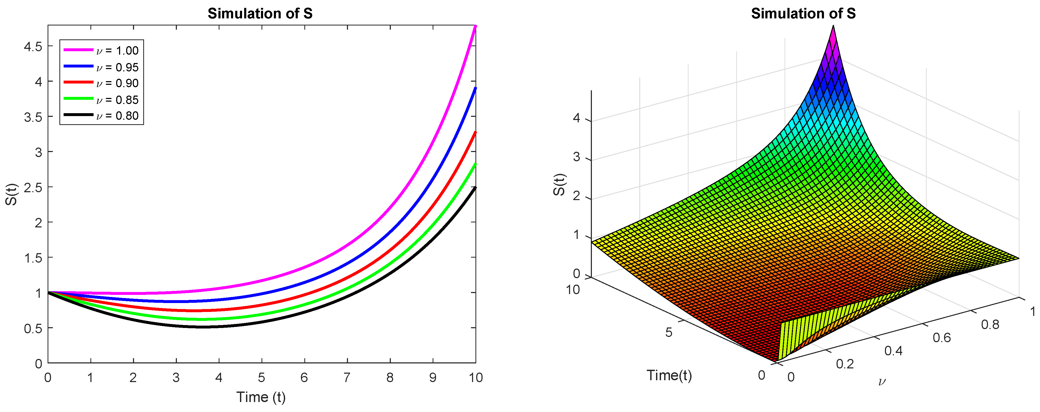
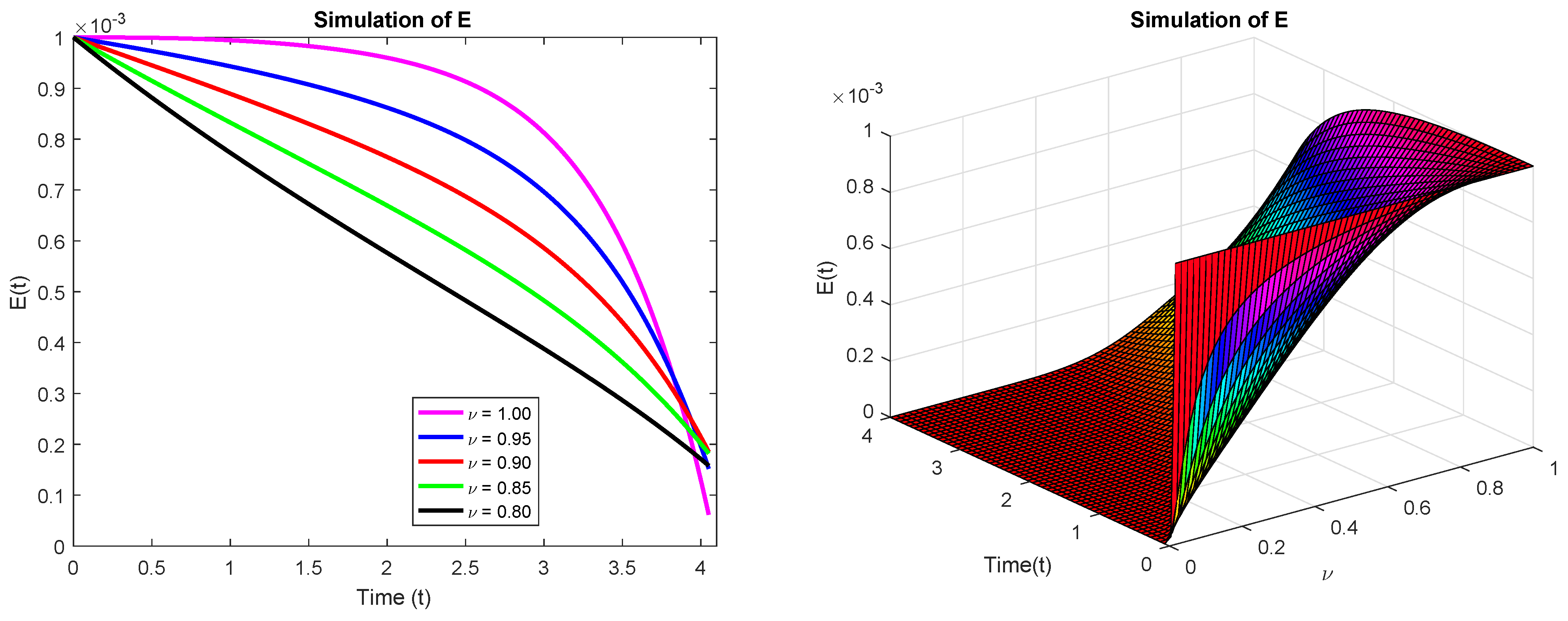
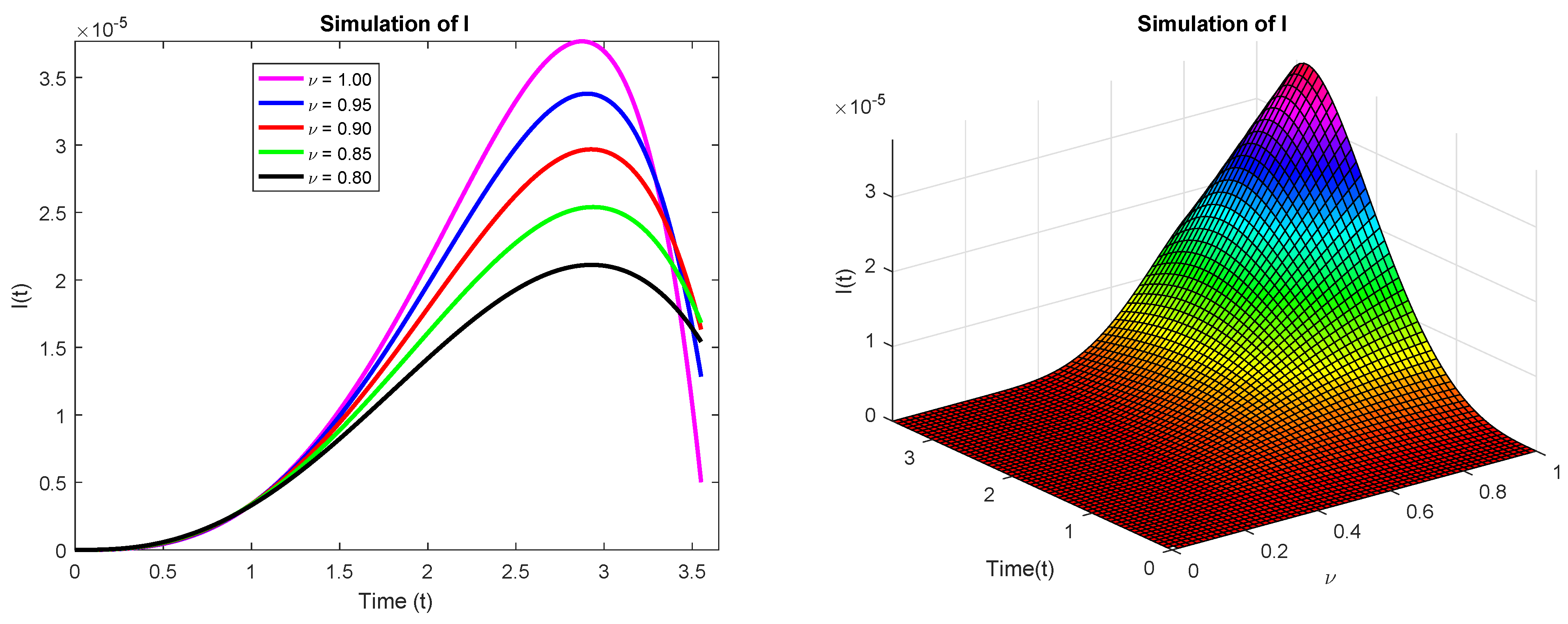
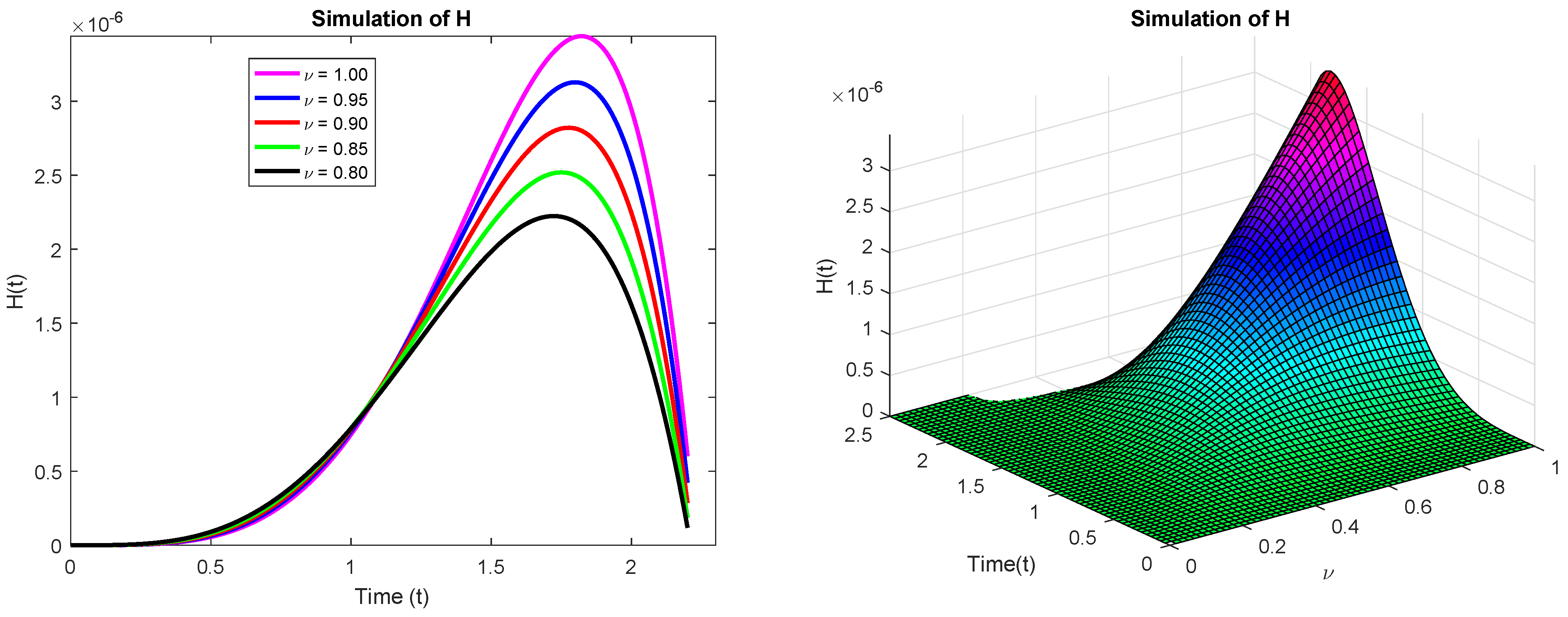
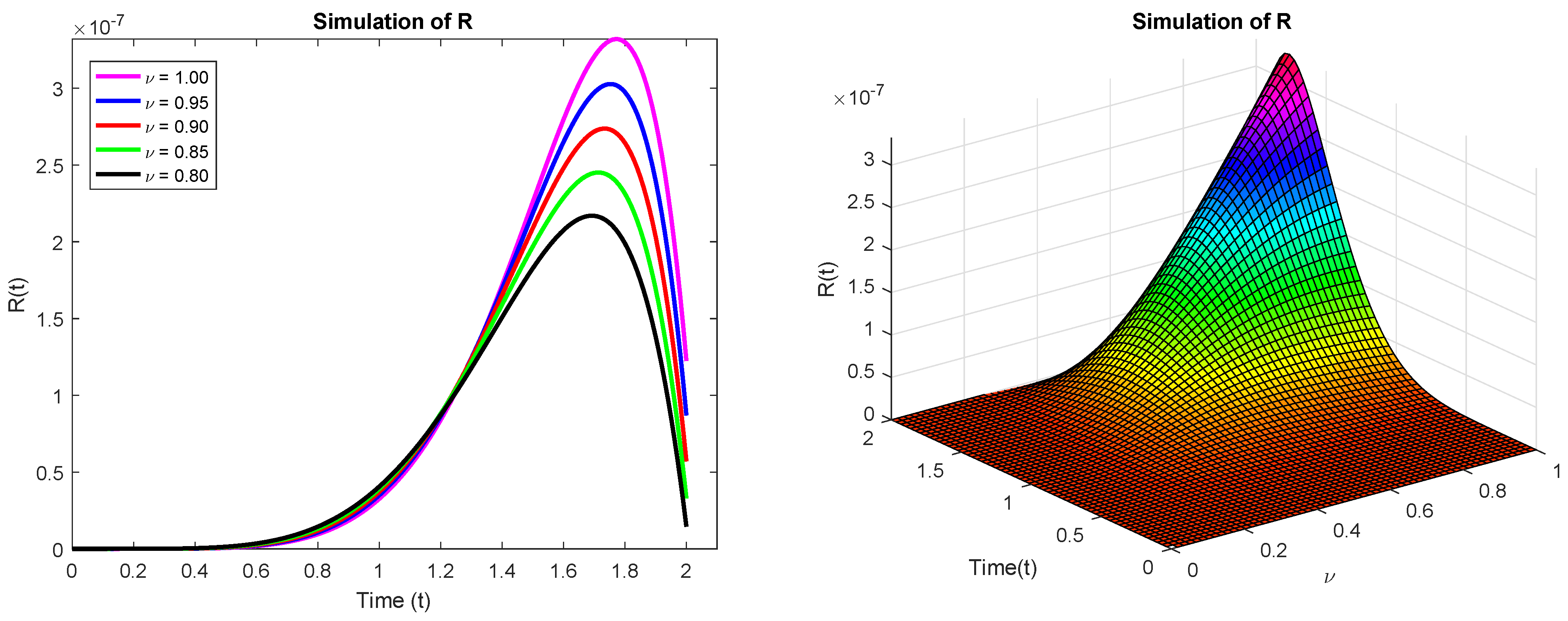
Figure 1, Figure 2, Figure 3, Figure 4, Figure 5 and Figure 6 are the representations of the susceptible people , exposed people , infected people , hospitalized people , recovered people , and dead people , respectively. As seen in Figure 1, the susceptible individuals rise as fractional values rise, whereas exposed , infected , hospitalized , recovered , and dead individuals fall as fractional values rise, as seen in Figure 2, Figure 3, Figure 4, Figure 5 and Figure 6, with all of the compartments of the proposed model convergent to their disease-free equilibrium. Additionally, we made use of 3D images to enhance the visualization of the simulation of the suggested model. By utilizing the model’s true geometry rather than condensing it to cylindric compartments, 3-D models are able to concurrently capture the Ebola virus potential and extracellular potential during activity. When fractional values are reduced, the behavior seen in every figure changes, suggesting that the outcome would be better if the fractional orders were lower than those of the integer-order derivative. Longer terms improve the approach’s effectiveness, while smaller fractional values improve the method’s accuracy and dependability. Graphical results show the spatiotemporal spread of the virus and the impacts of the vector sections by illustrating the memory influence of the fractional derivative in contrast with the traditional derivative. We find that the proposed fractional order structure is, in some ways, more flexible than ordinary derivatives. The trajectory of individuals changes more quickly for low fractional orders than for high fractional orders when values for fractions are present because they promote sectional cooperation. Table 3, Table 4, Table 5, Table 6, Table 7 and Table 8, which display the numerical results of several compartments, indicate bounds to disease-free spots at various fractional-order values over the course of a finite period of time.
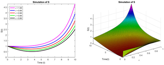
Figure 1.
Simulation of under different fractional orders .
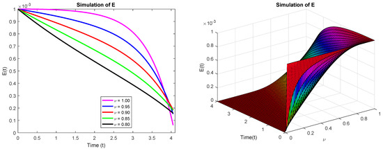
Figure 2.
Simulation of under different fractional orders .

Figure 3.
Simulation of under different fractional orders .
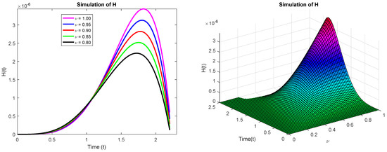
Figure 4.
Simulation of under different fractional orders .
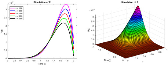
Figure 5.
Simulation of under different fractional orders .
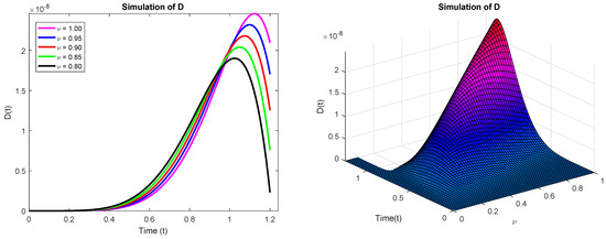
Figure 6.
Simulation of under different fractional orders .
Table 3.
Numerical simulation of for various fractional orders .
Table 4.
Numerical simulation of for various fractional orders .
Table 5.
Numerical simulation of for various fractional orders .
Table 6.
Numerical simulation of for various fractional orders .
Table 7.
Numerical simulation of for various fractional orders .
Table 8.
Numerical simulation of for various fractional orders .
7. Conclusions
In this study, our proposed Ebola virus model was examined using a nonlinear fractional-order model with a CPC derivative. It addressed the uniqueness of the claimed results using fixed-point theory discoveries, and it provided stable results for the fractional model using Ulam–Hyers conceptions. Theoretical and numerical data were offered for the proposed Ebola virus model, and the Laplace–Adomian decomposition method was used to arrive at the numerical results. The dynamics of infection are better understood by simulations, which also shows how the value of can affect a system’s behavior. To help public health professionals and decision-makers stop the spread of the Ebola virus, our fractional-order model analyzes the afflicted character from beginning to end. Our simulation demonstrates the evolution of an infected person’s health over time. As a result, this research is crucial for making decisions and setting boundaries.
Author Contributions
Methodology, C.X. and M.F.; Software, M.F.; Formal analysis, C.X. and M.F.; Investigation, C.X. and M.F.; Writing—original draft, C.X. and M.F.; Writing— review & editing, C.X. and M.F.; Project administration, M.F.; Funding acquisition, C.X. All authors have read and agreed to the published version of the manuscript.
Funding
Funding was provided by the Foundation of Science and Technology of Guizhou Province ([2019]1051) and the Guizhou University of Finance and Economics (2018XZD01).
Data Availability Statement
Not applicable.
Conflicts of Interest
The authors declare no conflict of interest.
References
- Ivorra, B.; Ngom, D.; Ramos, Á.M. Be-codis: A mathematical model to predict the risk of human diseases spread between countries-validation and application to the 2014–2015 ebola virus disease epidemic. Bull. Math. Biol. 2015, 77, 1668–1704. [Google Scholar] [CrossRef] [PubMed]
- Rachah, A.; Torres, D.F. Mathematical modelling, simulation, and optimal control of the 2014 Ebola outbreak in West Africa. Discrete dynamics in nature and society. Discret. Dyn. Nat. Soc. 2015, 2015, 1–9. [Google Scholar] [CrossRef]
- Djiomba, N.; Nyabadza, S.D.F. An optimal control model for Ebola virus disease. J. Biol. Syst. 2016, 24, 29–49. [Google Scholar] [CrossRef]
- Khajanchi, S.; Sarkar, K.; Mondal, J.; Nisar, K.S.; Abdelwahab, S.F. Mathematical modeling of the COVID-19 pandemic with intervention strategies. Results Phys. 2021, 25, 104285. [Google Scholar] [CrossRef] [PubMed]
- Khajanchi, S.; Sarkar, K.; Mondal, J. Dynamics of the COVID-19 pandemic in India. arXiv 2020, arXiv:2005.06286. [Google Scholar]
- Tiwari, P.K.; Rai, R.K.; Khajanchi, S.; Gupta, R.K.; Misra, A.K. Dynamics of coronavirus pandemic: Effects of community awareness and global information campaigns. Eur. Phys. J. Plus 2021, 136, 994. [Google Scholar] [CrossRef]
- Khajanchi, S.; Sarkar, K.; Banerjee, S. Modeling the dynamics of COVID-19 pandemic with implementation of intervention strategies. Eur. Phys. J. Plus 2022, 137, 129. [Google Scholar] [CrossRef]
- Mondal, J.; Khajanchi, S. Mathematical modeling and optimal intervention strategies of the COVID-19 outbreak. Nonlinear Dyn. 2022, 109, 177–202. [Google Scholar] [CrossRef]
- Khajanchi, S.; Bera, S.; Roy, T.K. Mathematical analysis of the global dynamics of a HTLV-I infection model, considering the role of cytotoxic T-lymphocytes. Math. Comput. Simul. 2020, 180, 354–378. [Google Scholar] [CrossRef]
- Bera, S.; Khajanchi, S.; Roy, T.K. Dynamics of an HTLV-I infection model with delayed CTLs immune response. Appl. Math. Comput. 2022, 430, 127206. [Google Scholar] [CrossRef]
- Bhatter, S.; Jangid, K.; Kumawat, S.; Purohit, S.D.; Baleanu, D.; Suthar, D.L. A generalized study of the distribution of buffer over calcium on a fractional dimension. Appl. Math. Sci. Eng. 2023, 31, 2217323. [Google Scholar] [CrossRef]
- Singh, J.P.; Abdeljawad, T.; Baleanu, D.; Kumar, S. Transmission dynamics of a novel fractional model for the Marburg virus and recommended actions. Eur. Phys. J. Spec. Top. 2023, 1–11. [Google Scholar] [CrossRef]
- Xu, C.; Mu, D.; Liu, Z.; Pang, Y.; Aouiti, C.; Tunc, O.; Ahmad, S.; Zeb, A. Bifurcation dynamics and control mechanism of a fractional-order delayed Brusselator chemical reaction model. Match-Commun. Math. Comput. Chem. 2023, 89, 73–106. [Google Scholar] [CrossRef]
- Farman, M.; Akgül, A.; Abdeljawad, T.; Naik, P.A.; Bukhari, N.; Ahmad, A. Modeling and analysis of fractional order Ebola virus model with Mittag-Leffler kernel. Alex. Eng. J. 2022, 61, 2062–2073. [Google Scholar] [CrossRef]
- Zhang, L.; Addai, E.; Ackora-Prah, J.; Arthur, Y.D.; Asamoah, J.K.K. Fractional-order Ebola-Malaria coinfection model with a focus on detection and treatment rate. Comput. Math. Methods Med. 2022, 2022, 1–19. [Google Scholar] [CrossRef]
- Khan, F.M.; Ali, A.; Bonyah, E.; Khan, Z.U. The mathematical analysis of the new fractional order Ebola model. J. Nanomater. 2022, 2022, 1–12. [Google Scholar] [CrossRef]
- Shah, N.H.; Chaudhary, K. Analysis of the Ebola with a fractional-order model involving the Caputo-Fabrizio derivative. Songklanakarin J. Sci. Technol. 2023, 45, 69–79. [Google Scholar]
- Tosin, A.S.; Yemisi, O.; Olarenwaju, I.M.; Bala, A. Approximate Solution of a Fractional-Order Ebola Virus Disease Model with Contact Tracing and Quarantine. Appl. Math. Comput. Intell. 2023, 12, 30–42. [Google Scholar]
- Ndenda, J.P.; Njagarah, J.B.H.; Shaw, S. Influence of environmental viral load, interpersonal contact and infected rodents on Lassa fever transmission dynamics: Perspectives from fractional-order dynamic modelling. AIMS Math. 2022, 7, 8975–9002. [Google Scholar] [CrossRef]
- Yavuz, M.; Özköse, F.; Susam, M.; Kalidass, M. A new modeling of fractional-order and sensitivity analysis for hepatitis-b disease with real data. Fractal Fract. 2023, 7, 165. [Google Scholar] [CrossRef]
- Chu, Y.M.; Zarin, R.; Khan, A.; Murtaza, S. A vigorous study of fractional order mathematical model for SARS-CoV-2 epidemic with Mittag-Leffler kernel. Alex. Eng. J. 2023, 71, 565–579. [Google Scholar] [CrossRef]
- Kulakov, M.; Frisman, E. Clustering Synchronization in a Model of the 2D Spatio-Temporal Dynamics of an Age-Structured Population with Long-Range Interactions. Mathematics 2023, 11, 2072. [Google Scholar] [CrossRef]
- Farman, M.; Alfiniyah, C.; Shehzad, A. Modelling and analysis tuberculosis (TB) model with hybrid fractional operator. Alex. Eng. J. 2023, 72, 463–478. [Google Scholar] [CrossRef]
- Taneja, K.; Deswal, K.; Kumar, D.; Baleanu, D. Novel Numerical Approach for Time Fractional Equations with Nonlocal Condition. Numer. Algorithms 2023, 138, 1–21. [Google Scholar] [CrossRef]
- Farman, M.; Baleanu, D. Modeling and Analysis of Smokers Model with Constant Proportional Fractional Operators. In Proceedings of the 2023 International Conference on Fractional Differentiation and Its Applications (ICFDA), Ajman, United Arab Emirates, 14–16 March 2023; IEEE: New York, NY, USA, 2023; pp. 1–7. [Google Scholar]
- Farman, M.; Shehzad, A.; Akgül, A.; Baleanu, D.; Sen, M.D.L. Modelling and analysis of a measles epidemic model with the constant proportional Caputo operator. Symmetry 2023, 15, 468. [Google Scholar] [CrossRef]
- Ali, A.D.; Erturk, V.S.; Zeb, A.R.; Khan, R.A. Numerical solution of fractional order immunology and aids model via Laplace transform Adomian decomposition method. J. Fract. Calcul. Appl. 2019, 10, 242–252. [Google Scholar]
- Baleanu, D.; Aydogn, S.M.; Mohammadi, H.; Rezapour, S. On modelling of epidemic childhood diseases with the Caputo-Fabrizio derivative by using the Laplace Adomian decomposition method. Alex. Eng. J. 2020, 59, 3029–3039. [Google Scholar] [CrossRef]
- Sweilam, N.; Al-Mekhlafi, S.; Baleanu, D. A hybrid fractional optimal control for a novel Coronavirus (2019-nCov) mathematical model. J. Adv. Res. 2020, 32, 149–160. [Google Scholar] [CrossRef]
- Caputo, M. Linear models of dissipation whose Q is almost frequency independent—II. Geophys. J. Int. 1967, 13, 529–539. [Google Scholar] [CrossRef]
- Baleanu, D.; Diethelm, K.; Scalas, E.; Trujillo, J.J. Fractional Calculus: Models and Numerical Methods; World Scientific: Singapore, 2012; Volume 3. [Google Scholar]
- Anderson, D.R.; Ulness, D.J. Newly defined conformable derivatives. Adv. Dyn. Syst. Appl. 2015, 10, 109–137. [Google Scholar]
- Baleanu, D.; Fernandez, A.; Akgül, A. On a fractional operator combining proportional and classical differintegrals. Mathematics 2020, 8, 360. [Google Scholar] [CrossRef]
- Ahmed, I.; Kumam, P.; Jarad, F.; Borisut, P.; Jirakitpuwapat, W. On Hilfer generalized proportional fractional derivative. Adv. Differ. Equations 2020, 2020, 1–18. [Google Scholar] [CrossRef]
- Jarad, F.; Abdeljawad, T.; Alzabut, J. Generalized fractional derivatives generated by a class of local proportional derivatives. Eur. Phys. J. Spec. Top. 2017, 226, 3457–3471. [Google Scholar] [CrossRef]
- Seck, R.; Ngom, D.; Ivorra, B.; Ramos, Á.M. An optimal control model to design strategies for reducing the spread of the Ebola virus disease. Math. Biosci. Eng. 2021, 19, 1746–1774. [Google Scholar] [CrossRef]
- Driessche, P.v.D.; Watmough, J. Reproduction numbers and sub-threshold endemic equilibria for compartmental models of disease transmission. Math. Biosci. 2002, 180, 29–48. [Google Scholar] [CrossRef] [PubMed]

Disclaimer/Publisher’s Note: The statements, opinions and data contained in all publications are solely those of the individual author(s) and contributor(s) and not of MDPI and/or the editor(s). MDPI and/or the editor(s) disclaim responsibility for any injury to people or property resulting from any ideas, methods, instructions or products referred to in the content. |
© 2023 by the authors. Licensee MDPI, Basel, Switzerland. This article is an open access article distributed under the terms and conditions of the Creative Commons Attribution (CC BY) license (https://creativecommons.org/licenses/by/4.0/).