Abstract
The time dynamics of the instrumental seismicity recorded in the area of the Lai Chau reservoir (Vietnam) between 2015 and 2021 were analyzed in this study. The Gutenberg–Richter analysis of the frequency–magnitude distribution has revealed that the seismic catalog is complete for events with magnitudes larger or equal to 0.6. The fractal method of the Allan Factor applied to the series of the occurrence times suggests that the seismic series is characterized by time-clustering behavior with rather large degrees of clustering, as indicated by the value of the fractal exponent . The time-clustering of the time distribution of the earthquakes is also confirmed by a global coefficient of variation value of 1.9 for the interevent times. The application of the correlogram-based periodogram, which is a robust method used to estimate the power spectrum of short series, has revealed three main cycles with a significance level of (of 10 months, 1 year, and 2 years) in the monthly variation of the mean water level of the reservoir, and two main periodicities with a significance level of (at 6 months and 2 years) in the monthly number of earthquakes. By decomposing the monthly earthquake counts into intrinsic mode functions (IMFs) using the empirical decomposition method (EMD), we identified two IMFs characterized by cycles of 10 months and 2 years, significant at the 1% level, and one cycle of 1 year, significant at the 5% level. The cycles identified in these two IMFs are consistent with those detected in the water level, showing that, in a rigorously statistical manner, the seismic process occurring in the Lai Chau area might be triggered by the loading–unloading operational cycles of the reservoir.
1. Introduction
Reservoir-triggered seismicity (RTS) is one of the main debated topics in seismology due to its potential to damage buildings and infrastructures and, in the worst cases, result in casualties. The RTS phenomenon is linked to several factors, including static loading (such as the weight of the water reservoir and seasonal changes in the water level), tectonic faults, liquefaction, and variations in pore pressure. Numerous studies have investigated RTS, including references [1,2,3,4,5,6,7,8,9,10]. These studies generally concluded that the impoundment of a reservoir affects the Earth’s crust and influences the seismic activity in regions prone to earthquakes. The operation of a reservoir typically follows a cyclic loading pattern driven by the seasonal fluctuations of the water level, as discussed in reference [3]. Previous research has suggested that RTS may be related to pore pressure diffusion beneath the reservoir or the gravitational loading of the reservoir, as proposed in [11,12,13]. Mikhailov et al. [5] suggested that earthquakes could be triggered by a combination of factors, including ambient stress field conditions resulting from water loading to a failure, hydromechanical properties of rocks beneath the reservoir, local geology, reservoir size, and fluctuations of lake levels. Rajendran et al. [14] identified triggered seismicity as a consequence of the disruption of equilibrium caused by a reduction in the strength of fault zones. This conclusion was further refined by the authors of reference [1], who asserted that “water passes through the basalts broken by the meridional faults and penetrates into the fault zone with the highly permeable” layers. There are documented cases of seismic activity occurring in aseismic regions globally, years after the impoundment of a reservoir, as observed by Malik et al. [15].
In Vietnam, the occurrence of earthquakes in the vicinity of the Hoa Binh hydropower reservoir in 1989 prompted seismological researchers to focus on studies on reservoir-triggered seismic activity. The construction of the Hoa Binh hydropower was accomplished in 1988 and the reservoir was impounded in May 1988. But on 23 May 1989, a large earthquake with a magnitude of occurred in the area of the reservoir, leading researchers to suggest the event was triggered by the reservoir [16,17]. After the Hoa Binh reservoir, the impoundment of the Song Tranh 2 reservoir began, and soon after, in March 2011, seismic activity increased in its vicinity, culminating in two large earthquakes with local magnitudes of 4.6 and 4.7 on 22 October and 15 November 2012, respectively.
The impact of the stress field, caused by reservoir load on the fault plane, was investigated to gain insights into the causative mechanisms of earthquakes in this region [18,19]; previous research was conducted to explore the connection between changes in the water level of the reservoir and seismic activity by using robust statistical techniques [20,21,22].
The Lai Chau reservoir is located in the Lai Chau province in northwestern Vietnam. Construction of the dam commenced on 5 November 2011, at the upper reaches of the main Da River in Vietnam, near the border with China. The dam’s highest point reaches an elevation of 303 m, and it has a total capacity of 1215 million cubic meters. The impoundment of the Lai Chau hydropower reservoir took place in June 2015. Lizurek et al. [23] conducted research to assess the earthquake’s background before and after the reservoir impoundment. Additionally, Wiszniowski et al. [24] employed machine learning and artificial intelligence techniques to automatically detect earthquake signals in waveform data and determine earthquake locations. However, up until this point, no comprehensive study has been undertaken to conclusively analyze triggered seismicity in the region.
In this work, we analyze seismicity around the Lai Chau reservoir by using several statistical methods (fractal, spectral, and decompositional) to deeply investigate the series of earthquakes and assess their potential relationship with the cyclic operational activity of the dam.
2. Seismotectonic Settings
Northwestern Vietnam is a mountainous region with a complicated geological structure, dominated by many active faults, such as the Lai Chau–Dien Bien Fault zone, the Son La Fault, the Ma River Fault, the Da River Fault zone, and the Red River Fault. This region is the most seismically active in Vietnam. The present tectonic features of the faults are determined on the basis of surface geological investigations and studies of deep crustal structures [18,25,26,27,28]. The Lai Chau reservoir is located in the Muong Te district, the Lai Chau province of northwestern Vietnam, and the dam was constructed on the Paleozoic rocks of the Da River complex formations (Figure 1) [27,28]. There are four main faults in the studied region: Lai Chau–Dien Bien, Muong Te, Nam Nho, and Nam Nhe; all the remaining faults are branches of these main faults. The Lai Chau–Dien Bien is the most active fault zone in the study region; the strongest earthquakes (M > 5) were observed on this fault zone. This fault zone was formed in the early–middle Jurassic period (198–158 Ma) during its first deformation phase. Since then, the fault zone has undergone several deformation phases; presently, the fault exhibits left-lateral and normal left-lateral motions, with the normal component increasing towards the north [28]. The Muong Te fault zone, near which the Lai Chau reservoir is located, has two deformation phases in the neotectonic period: the early phase of the left-lateral strike-slip motion and the late phase of the right-lateral strike-slip motion. Moderate earthquakes () were observed at this fault zone. Similar to the Muong Te fault zone, the Muong Nhe fault zone also has two deformation phases, the left and right-lateral strike-slip motions in the early and late phases, respectively. Small earthquakes were observed at the Muong Nhe and Nam Nhe fault zones (Figure 1) [27,28,29].
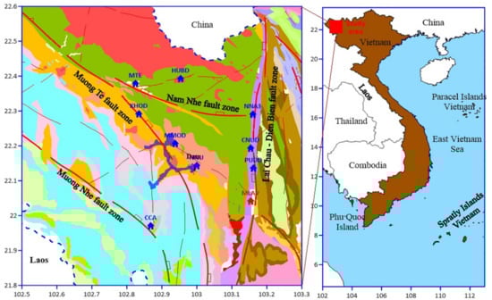
Figure 1.
Seismotectonics of northwestern Vietnam. The local seismic stations and national seismic stations are denoted by blue and red symbols, respectively. The geology and geologically identified mapped faults (red) with dip and slip directions are taken from [29].
Before September 2014, the seismicity of the Lai Chau region was monitored by the Vietnamese National Stations Network, which could record earthquakes at a magnitude of . Only the Muong Lay (MLAV) station of this network was located in the Lai Chau region (the red symbol in Figure 1). From September 2014 to June 2017, a seismic network of nine stations was established by the Institute of Geophysics, the Vietnam Academy of Science and Technology (IGP-VAST). The stations are situated on hard rock. Among these, Nam Nhun (NNU), Muong Te (MTE), Nam Na 3 (NNA3), and Cha Cang (CCA) were equipped with Guralp-CMG-6TD seismometers; Chan Nua (CNUD), Pu Dao (PUDD), Muong Mo (MMOD), Can Ho (KHOD), and Hua Bum (HUBD) are equipped with GeoSIG-GMSplus seismometers [23]. All stations have a sampling rate of 100 samples per second. The positions of stations are determined based on the locations of previous earthquakes, ensuring the recordings of small earthquakes around the reservoir. A system based on SeisComP software (http://www.seiscomp.de/) was used for data collection. Additional components, like modules for communicating with stations, were added to adapt the system to the project’s requirements. Data from Guralp stations were downloaded using the SCREAM program and then transmitted to SeisComP. The earthquake data were analyzed using the SEISAN seismic analysis software (https://www.seisan.com/). The continuous waveform data from the nearest stations were first analyzed and the timings of the local earthquakes were noted; the particular waveforms of those earthquakes were picked up from the rest of the seismic stations. The waveforms of a particular earthquake from all the stations were merged to determine the hypocenter parameters, i.e., the origin times, locations, focal depths, magnitudes, and errors in these four parameters.
3. The Frequency–Magnitude Distribution
The Gutenberg–Richter (GR) law [30] that correlates the number N of earthquakes of magnitude to the magnitude threshold and is represented by is generally used to fit the frequency–magnitude distribution of earthquakes. The a-value indicates the level of seismicity or “seismic productivity” in an area and the b-value provides information about the proportion of small events compared to large ones and the stress conditions of the crust. The reliable estimate of the b-value, then, is necessary to perform a reliable assessment of seismic hazards (Scholz, 1968; Wyss, 1973). In this study, we apply the maximum likelihood method (MLE) [31] to estimate the b-value:
where is the average magnitude of the subset of earthquakes of magnitude , where is the binning width of the catalog and is the completeness magnitude, which is the minimum magnitude that could be detected by the seismic network [32].
The estimate of the b-value depends on the calculation of . We employ the goodness-of-fit test (GFT) method [33] to calculate . By using the GFT method, is calculated by comparing the observed frequency–magnitude distributions with synthetic ones. The synthetic distributions are obtained using the values of a and b, estimated from the observed dataset for magnitude as the function of the increasing cutoff magnitude . Let R represent the absolute difference in the number of earthquakes in each magnitude bin between the observed and synthetic distributions, is found at the first , for which the observed data for are modeled by a straight line (in log–lin plot) for a fixed confidence level . Lizurek et al. [23] examined seismic activity in a region spanning several tens of kilometers from the center of the dam, and reported a completeness magnitude of 0.7 and a b-value of 0.5 after the impoundment of the dam.
In this paper, we analyzed the series of earthquakes that occurred around the Lai Chau water reservoir (Vietnam) from 2015 to 2021, within 10 km of the center of the dam (Figure 2). The maximum depth of the hypocenters is 8.8 km and the number of events is 136.
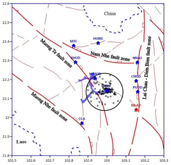
Figure 2.
Spatial distribution of the analyzed seismicity. The earthquakes included in the black circle are located within 10 km from the center of the reservoir.
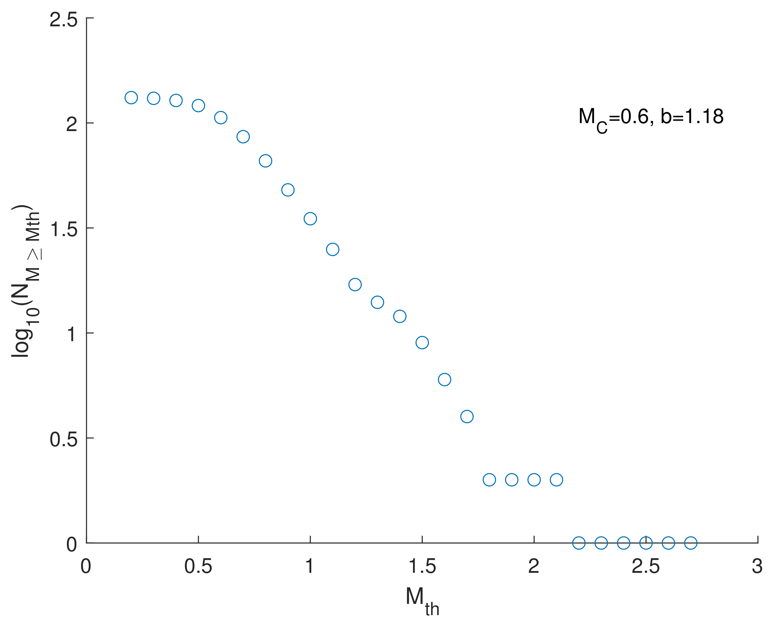
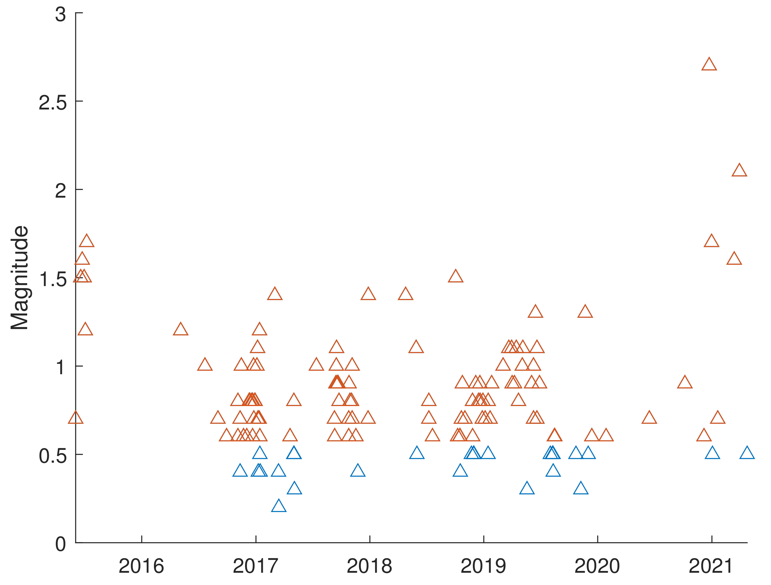
Prior to examining the fractal and spectral characteristics of the seismic dataset, we computed the frequency–magnitude distribution (Figure 3) and utilized the GFT (goodness-of-fit test) method with a confidence level of to determine the completeness magnitude, which was found to be . By using Equation (1), we obtained a b-value of 1.18. Thus, we only selected those earthquakes of magnitude , which reduced the total number of earthquakes to 106 (represented by the red triangles in Figure 4). Subsequent analyses will be conducted on this complete subset of earthquakes.
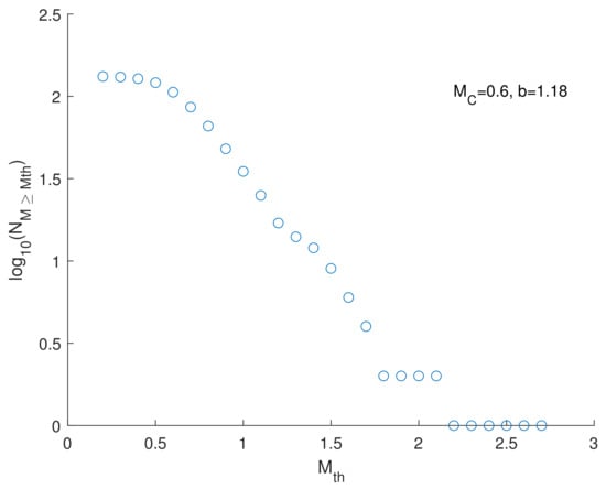
Figure 3.
Cumulative frequency–magnitude distribution. By applying the GFT method the completeness magnitude = 0.6 and b = 1.18.
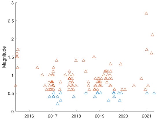
Figure 4.
Time distribution of the earthquakes in the investigated area. The red triangles represent the earthquakes above the completeness magnitude.
4. Methods
4.1. The Allan Factor
A seismic sequence can be described by a temporal point process marked by the magnitude
where is the occurrence time of the earthquake i with magnitude .
Dividing the time axis into equally spaced contiguous windows with a duration of (representing the timescale), the series of earthquake counts can be constructed, counting the number of events that fall in each k-th window [34].
AF is defined by the following formula:
where the symbol indicates the mean. AF was used to investigate the time dynamics of a variety of natural phenomena [35,36]. If the series of events are Poissonian, meaning that the events are uncorrelated and independent, AF is rather flat for all available timescales, fluctuating at around 1 (except for very large timescales due to finite-size effects [37]); if the series of events are clusterized, the AF changes with the timescale , increasing as a power law for a fractal (self-similar) process:
The power law exponent , called the fractal exponent, quantifies the strength of time-clustering; is the fractal onset time and delimits the lower limit of significant scaling behavior in the AF [34]. Thus, if , the earthquake sequence can be considered Poissonian, and if , it is clusterized.
For a purely periodic process, AF approaches zero as the timescale increases [38], with local minima corresponding to timescales multiple of the main period [39]; therefore, the timescale where the AF drops down corresponds to the periodicity.
In regard to Poissonian point processes, since the occurrence times are uncorrelated and independent, the probability density function of the interevent time is a decreasing exponential function , with denoting the mean rate of the process. In clusterized fractal point processes, the generally decreases as a power law function of the interevent time, , with denoting the above-mentioned fractal exponent [34]. As an example, Figure 5 shows two simulated sequences: a Poissonian (red) sequence and a fractal sequence with a scaling exponent of (blue), alongside their AF curves; the two sequences have the same number of events (consistent with the number of events of the Lai Chau area) and are generated to keep the same mean interevent time. By fitting the AF curve displayed in log-log scales with a line and determining the slope using the least squares method, the estimated scaling exponent of the fractal series is 0.47. This is remarkably close to the theoretical value of 0.5.
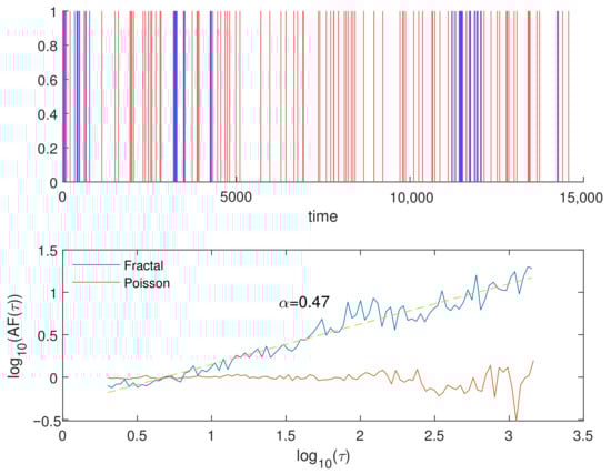
Figure 5.
(Top) Poissonian (red) and fractal (blue) simulated sequences of N = 100 events with a mean interevent time = 143.95. The fractal sequence was simulated with a fractal exponent = 0.5. (Bottom) the Allan Factor of the two sequences. The fractal sequence shows increasing behavior of the AF with an estimated scaling exponent = 0.47.
4.2. The Global and Local Coefficients of Variation
Representing a seismic sequence as the series of the interevent times, which are the intervals between consecutive events, we can define two quantities: the global coefficient of variation [40]:
and the local coefficient of variation [41]
where is the series of the interevent times and and are their standard deviation and mean.
These two quantities are used to quantify the time-clustering presence in a series of earthquakes. For Poissonian earthquake sequences, both and are 1, for periodic or regular sequences, they are lower than 1, while for clusterized sequences, they are larger than 1. measures the global clustering properties of the sequence and, thus, could be affected by event rate fluctuations, while measures the local stepwise variability of the interevent times, because it is rather independent of the slow variation in the average rate. For instance, by joining two periodic sequences, the resulting sequence is characterized by because it appears periodic locally. On a global scale, it could appear highly clusterized, with a larger than 1. By calculating and for the two simulated sequences shown in Figure 5, the Poissonian series yields and , while the fractal series produces and . These values confirm the purely random nature of the time distribution of the Poissonian sequence and the clusterized character of the fractal sequence on both global and local scales.
4.3. The Correlogram-Based Periodogram
Regarding short time series, an efficient algorithm to calculate the power spectrum is the correlogram-based periodogram. Telesca et al. [8] employed this method to detect the yearly cycle in the monthly and quarterly number of earthquakes that occurred around the Pertusillo Reservoir (Southern Italy). Considering the simple model of periodic series:
with > 0, , distributed as a uniform variable in , and denoting a series of uncorrelated random variables with a mean of 0 and standard deviation , independent of .
The classical periodogram is given by
with N being the length of the series, and it is calculated by
where , and indicates the integer part of x. If the series is modulated by a strong cycle with frequency , the periodogram shows a peak at . For an uncorrelated series, instead, , the periodogram is almost flat, without any clear peak [42]. Ahdesmäki et al. [43] proposed a correlogram-based periodogram that is more effective than the classical periodogram in detecting the main cycle of a series. The classical periodogram is equivalent to the correlogram:
where
is the estimator of the autocorrelation function. Using the sample autocorrelation function
where indicates the mean, Ahdesmäki et al. [43] proposed the following correlogram-based periodogram to estimate the power spectrum of a series:
where indicates the real part of x, N is the length of the series, and is the biased Spearman rank correlation coefficient. Contrary to the standard periodogram, the correlogram-based periodogram can be negative; thus, the absolute value is considered.
To test a frequency , the g-statistics can be used:
If g is large, then the tested frequency is very powerful. To evaluate the significance of the tested frequency, we can use the simulation-based technique [43]: random series modeled as Equation (7) are generated. For each simulated series, the g-value is calculated by using Equation (14). The distribution of g-statistics is estimated by all the calculated g-values and, therefore, the p-value is obtained. A low p-value identifies a strong frequency.
4.4. Empirical Mode Decomposition
Huang et al. [44] proposed the use of the empirical mode decomposition (EMD) to decompose a series into a finite and often small number of components, called intrinsic mode functions (IMFs). The IMFs satisfy the following two conditions: (1) the number of extremes and that of zero-crossings differ at most by one; (2) at any point, the mean value of the upper (defined by the local maxima) and lower (defined by the local minima) envelopes is zero. The decomposition of a series into the IMFs makes use of the sifting algorithm:
- (a)
- Identify all the local maxima and connect them with a cubic spline line to produce the upper envelope ;
- (b)
- Repeat a) for the local minima to produce the lower envelope ;
- (c)
- Calculate the mean and subtract it from the series: ;
- (d)
- If does not meet the criteria to be considered an IMF, treat as the series and return to (a). The sifting process will be repeated until an IMF is obtained.
- (e)
- After obtaining the first IMF , subtract it from the series and return to (a).
- (f)
- When all the IMFs are obtained, the residual is just given by removing from the series all the IMFs that were found.
The whole decomposition is expected to be completed with a finite number of IMFs.
5. Results
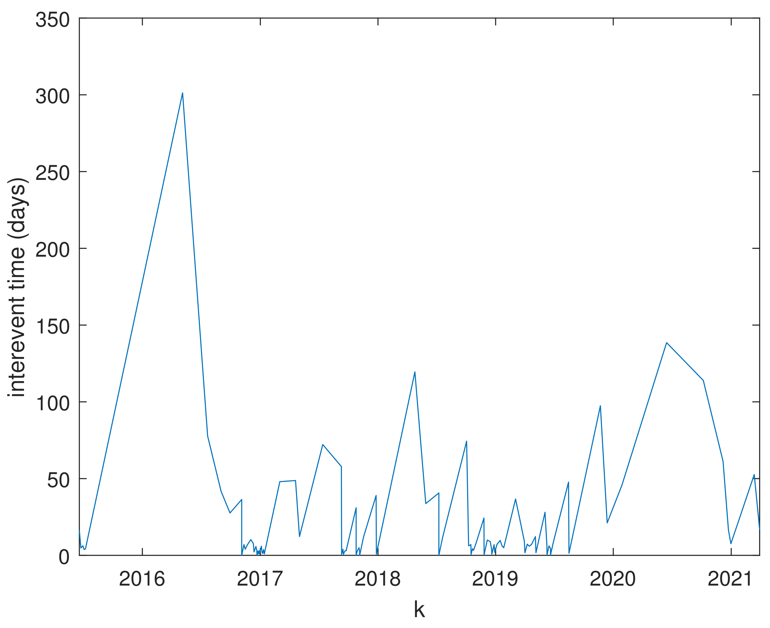
Our investigation focused on the fractal and spectral features of seismicity that occurred around the Lai Chau reservoir. Figure 6 shows the interevent times; the large interevent time values correspond to events that occurred after large periods in which no earthquakes occurred, while small values correspond to periods in which the earthquakes occurred as clusters. The series of interevent times allows one to calculate the global and local coefficients of variation, = 1.9 and = 1.14; these values indicate that the seismic series is globally clusterized in time much more than locally. The relatively large value of and low value of , rather close to the Poissonian limit, indicate that the series of earthquakes can be viewed as a superposition of clusters, with earthquakes behaving as a Poisson process within each of them.
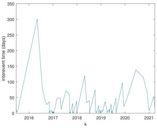
Figure 6.
Interevent times of the analyzed earthquakes.
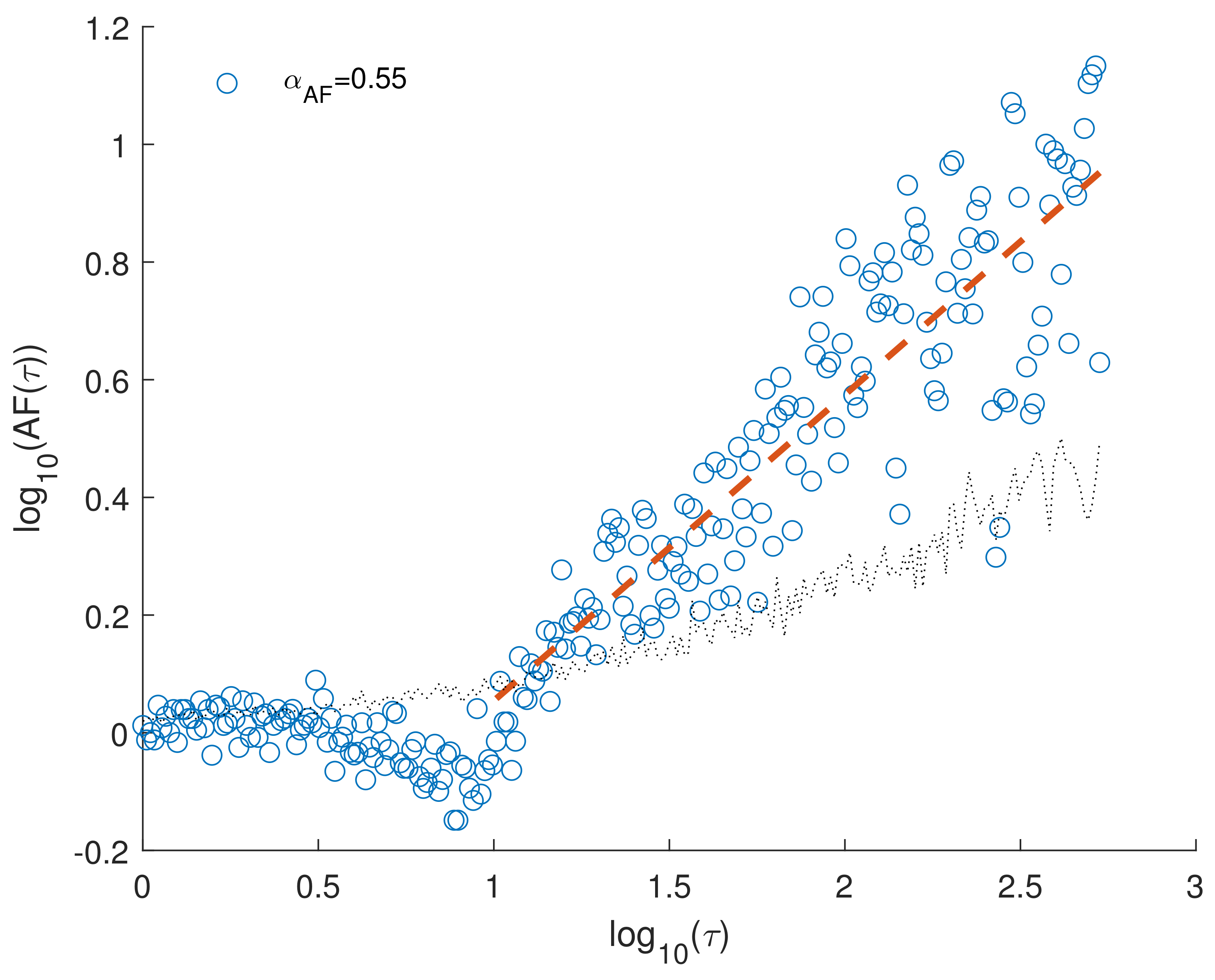
Figure 7 illustrates the AF of the earthquake series, represented by blue circles. The AF consistently exceeds the 97.5% confidence curve for a Poissonian distribution (depicted as a black dotted line), signifying a significant temporal clustering within the earthquake series. To derive the Poissonian 97.5% confidence curve, we generated one thousand Poissonian surrogates with the same number of events and mean interevent time as the original earthquake sequence. For each surrogate, we calculated the AF, and at each timescale , we computed the 97.5 percentiles from their AF values. Consequently, the 97.5% confidence curve was constructed by enveloping these 97.5 percentiles.
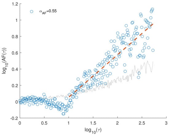
Figure 7.
The Allan factor of the analyzed earthquake series in log–log scales (blue circle). The dotted gray line represents the 95% confidence line for Poisson surrogates (see the text for details). The red dashed line is the least-squares linear fitting function for timescale > 10 days. The AF scaling exponent is the slope of the fitting line.
When examining the AF using a log–log scale, we observed a mostly linear increase for timescales exceeding approximately 10 days, which we consider the cutoff timescale. Below this threshold, the seismic process can be approximated as Poissonian. By fitting the log–log representation of AF for using the least squares method, we determine a scaling exponent value of . This suggests a rather high degree of temporal clustering within the earthquake series. Although the AF exhibits some scatter within the range of timescales used for estimating the scaling exponent , the overall increasing trend of AF with increasing indicates that the earthquake series displays fractal temporal distribution.
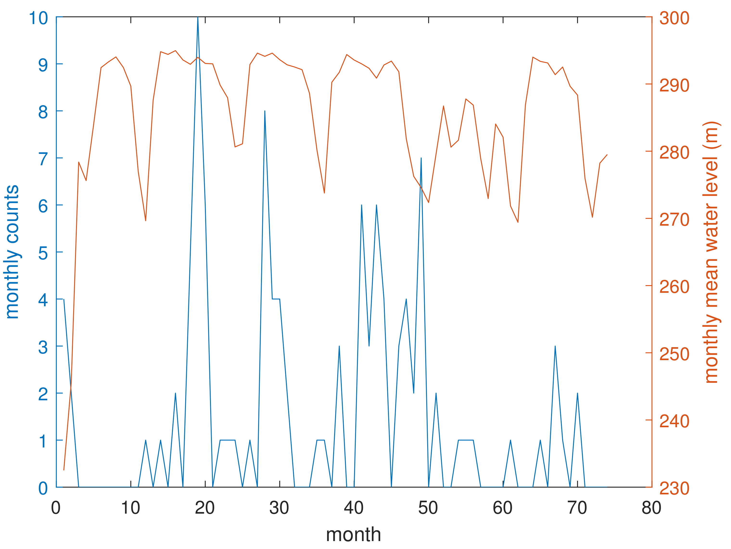
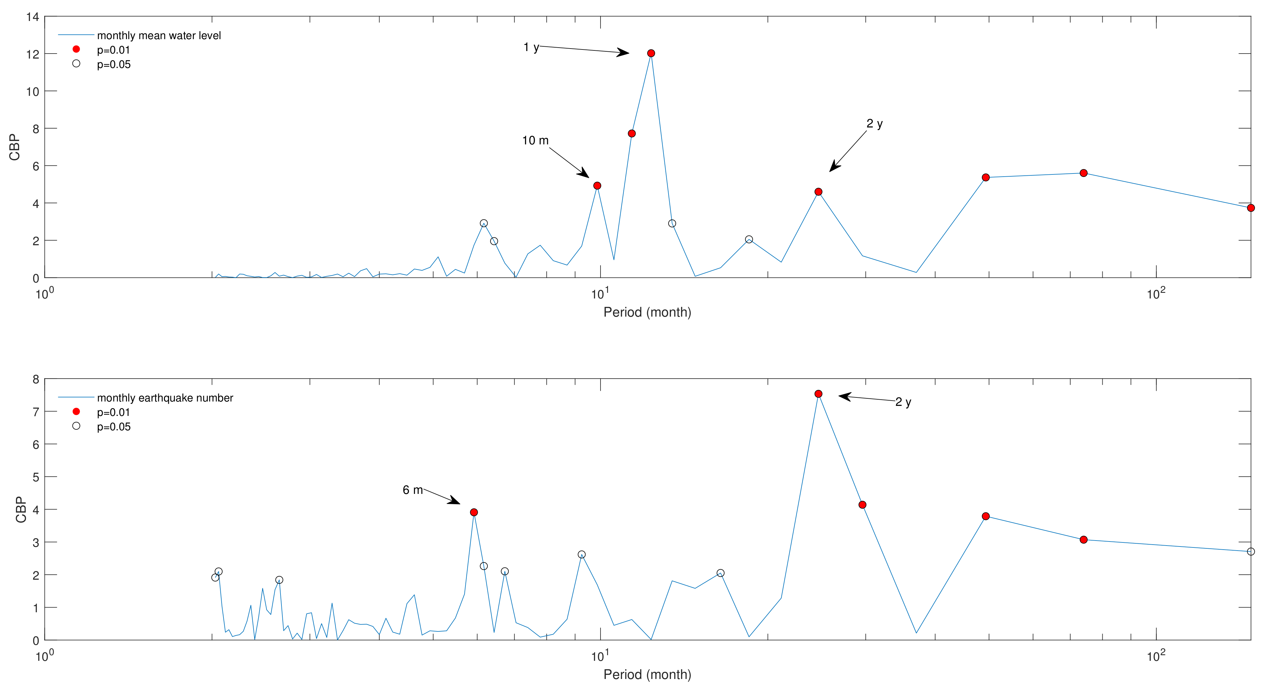
Figure 8 depicts the monthly variations in the number of earthquakes (with ) alongside the mean water level of the Lai Chau reservoir. In Figure 9, we present the correlogram-based periodogram for both series. The marked points in the periodogram denote periods significant at p below 0.05 (indicated by black hollow circles) and below 0.01 (indicated by red filled circles).
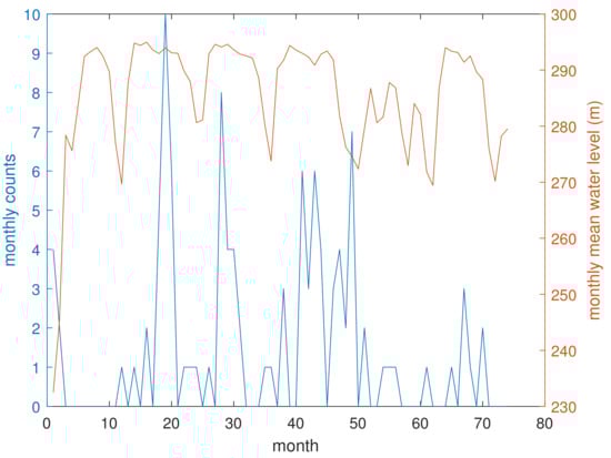
Figure 8.
Monthly number of earthquakes and mean water level of the Lai Chau reservoir.
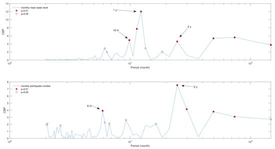
Figure 9.
Correlogram-based periodogram for the monthly mean water level and number of earthquakes. The black hollow circles mark the periodicities significant at , while the filled red circles mark the periodicities significant at .
When considering periodicities significant at p < 0.01, we observe that the monthly mean water level exhibits three main periodicities (10 months, 1 year, and 2 years). On the other hand, the monthly number of earthquakes displays two main cycles at 6 months and 2 years. Notably, the peak at 1 year in the mean water level is the most prominent, which aligns with the annual loading/unloading cycles of the reservoir, and is consistent with the region’s climatology. Additionally, the presence of a peak at 2 years in the correlogram-based periodogram of the monthly number of earthquakes suggests that the seismic activity is primarily influenced by a biannual oscillation, which may be related to the biannual cycle of the mean water level. It should be highlighted that a periodicity or cycle corresponds to a peak in the periodogram. In fact, if we look at the correlogram-based periodogram of the water level, for instance, the period between 1 year and 10 months, despite being significant with p < 0.01, cannot be considered a cycle because it is not a peak of the periodogram; the three periods above 2 years, significant with p < 0.01, do not qualify as cycles, rather, they reflect the long-term fluctuations in the water level.
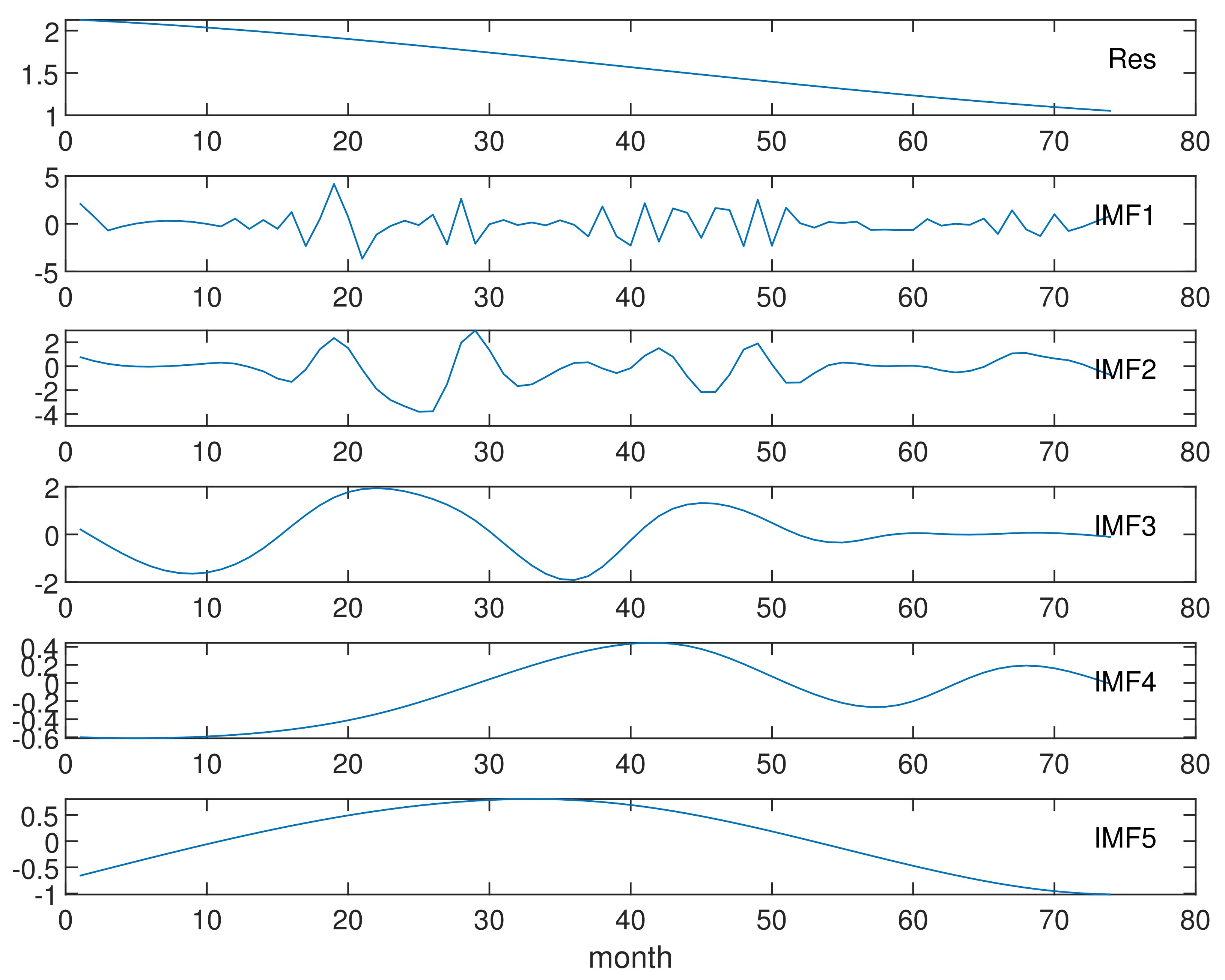
In order to delve deeply into the insights and time dynamics of the earthquakes, and to possibly find out the fingerprints of the yearly cycle (that could be put in a relationship with the annual loading/unloading cycles of the reservoir), we employed the empirical mode decomposition (EMD) method on the count series. The sifting algorithm generated five intrinsic mode functions (IMFs) and a residual component, as visualized in Figure 10. Subsequently, we computed correlogram-based periodograms for each IMF, as presented in Figure 11.
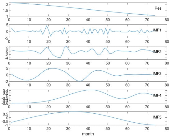
Figure 10.
Residuals and IMFs of the EMD applied to the monthly number of earthquakes.
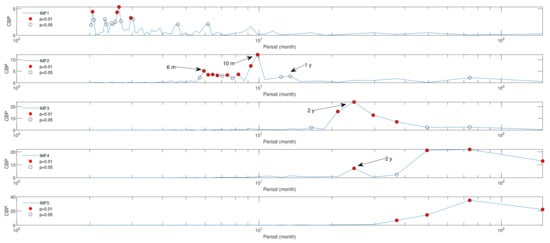
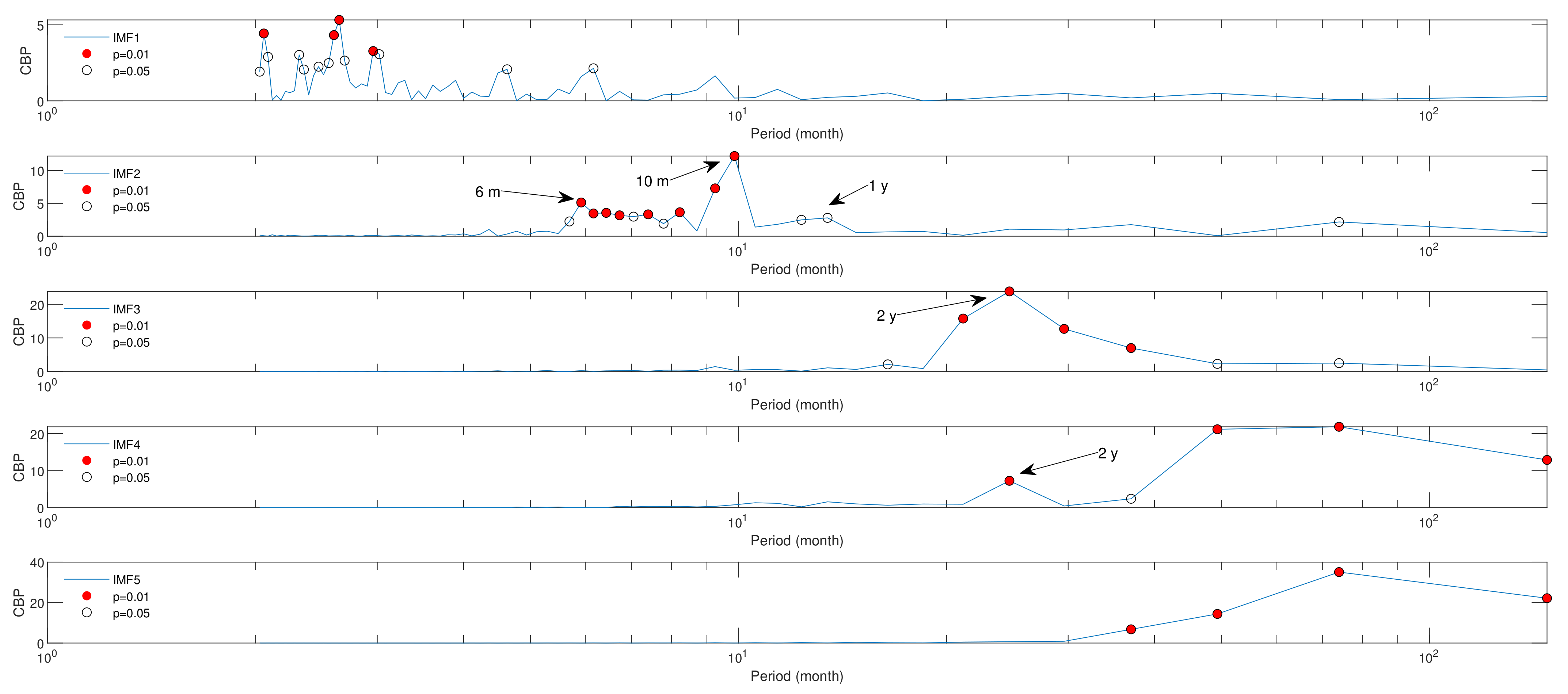
Figure 11.
Correlogram-based periodogram for the IMFs of the monthly number of earthquakes. The black hollow circles mark the periodicities significant at , while the filled red circles mark the periodicities significant at .
Among these five IMFs, the second one exhibits significant periodicities at the 1% significance level with a cycle of 10 months, and at the 5% significance level with an annual cycle; a further period appears significant at the 1% significance level with a cycle of 6 months, which could likely be considered a higher harmonic of the annual periodicity. Meanwhile, the third and fourth IMFs reveal significant periodicities at the 1% significance level, with a cycle of 2 years. The correlogram-based periodogram of the first IMF is predominantly marked by higher content at shorter periods ranging between 2 and 3 months, suggesting that it predominantly captures the short-term fluctuations within the count series. In contrast, the fifth IMF is indicative of the series’ long-term variations, as evidenced by its correlogram-based periodogram, which exhibits higher content at relatively longer periods. The identified periodicities in the EMD components of the monthly counts, in particular, the ones of 10 months and 2 years with a significance level of 1%, and at 1 year with a significance level of 5%, align with the principal significant periodic patterns that characterize the oscillatory fluctuations in water levels. This suggests that seismic activity around the Lai Chau reservoir may be influenced, in part, by the loading and unloading cycles of the reservoir.
6. Conclusions
In this paper, we analyzed the temporal dynamics of the instrumental seismic activity that occurred between 2015 and 2021 in the vicinity of the Lai Chau reservoir in Vietnam. Our analysis focused on a dataset comprising seismicity located within a maximum distance of 10 km from the reservoir’s center and reached depths of up to about 9 km. The goal of our study was to deeply investigate the time dynamics of seismicity by using fractal and spectral methods. Additionally, the use of the EMD has allowed us to decompose the series of earthquake counts into independent components, capturing short-term as well as long-term fluctuations of the series, along with the identification of annual and biannual periodicities that might be associated with fluctuations in the water level of the reservoir.
Author Contributions
Conceptualization, L.T.; methodology, L.T.; software, L.T.; formal analysis, L.T.; investigation, L.T., A.T.T. and D.T.C. (Dinh Trong Cao); resources, L.T. and A.T.T.; data curation, A.T.T., D.T.C. (Dinh Trieu Cao), Q.V.D. and X.B.M.; writing—original draft preparation, L.T.; writing—review and editing, L.T. and A.T.T.; visualization, L.T. and A.T.T.; project administration, L.T. and D.T.C. (Dinh Trong Cao); funding acquisition, L.T. and D.T.C. (Dinh Trong Cao). All authors have read and agreed to the published version of the manuscript.
Funding
This research was funded by the Vietnam Academy of Science and Technology (VAST) under grant number VAST05.02/23-24, the CNR-VAST Italy–Vietnam common project 2023–2024 under grant number QTIT01.02/23-24, the Institute of Geophysics–VAST under grant number CSCL12.01/23-24, and the Ministry of Science and Technology of Vietnam under grant number DTDLCN.58/22.
Data Availability Statement
Not applicable.
Conflicts of Interest
The authors declare no conflict of interest.
References
- Rajendran, K.; Harish, C.M. Mechanism of triggered seismicity at Koyna: An assessment based on relocated earthquake during 1983–1993. Curr. Sci. 2000, 79, 358–363. [Google Scholar]
- do Nascimento, A.F.; Cowie, P.A.; Lunn, R.J.; Pearce, R.G. Spatio-temporal evolution of induced seismicity at Acu reservoir, NE Brazil. Geophys. J. Int. 2004, 158, 1041–1052. [Google Scholar] [CrossRef]
- Gupta, H.; Shashidhar, D.; Pereira, M.; Purnachandra Rao, N.; Kousalya, M.; Satyanarayana, H.V.S.; Saha, S.; Babu Naik, R.T.; Dimri, V.P. A new zone of seismic activity at Koyna, India. J. Geol. Soc. India 2007, 69, 1136–1137. [Google Scholar]
- Gupta, H.K.; Rao, N.P.; Roy, S.; Arora, K.; Tiwari, V.M.; Patro, P.K.; Satyanarayana, H.V.S.; Shashidhar, D.; Mallika, K.; Akkiraju, V.V. Investigations related to scientific deep drilling to study reservoir triggered earthquakes at Koyna, India. Int. J. Earth Sci. (Geol. Rundsch.) 2015, 10, 1511–1522. [Google Scholar] [CrossRef]
- Mikhailov, V.O.; Arora, K.; Ponomarev, A.V.; Srinagesh, D.; Smirnov, V.B.; Chadha, R.K. Reservoir induced seismicity in the Koyna–Warna region, India: Overview of the recent results and hypotheses. Izv. Phys. Solid Earth 2017, 53, 518–529. [Google Scholar] [CrossRef]
- Valoroso, L.; Improta, L.; Chiaraluce, L.; Di Stefano, R.; Ferranti, L.; Govoni, A.; Chiarabba, C. Active faults and induced seismicity in the Val d’Agri area (Southern Apennines, Italy). Geophys. J. Int. 2009, 178, 488–502. [Google Scholar] [CrossRef]
- Braun, T.; Cesca, S.; Kuhn, D.; Martirosian-Janssen, A.; Dahm, T. Anthropogenic seismicity in Italy and its relation to tectonics: State of the art and perspectives. Anthropocene 2018, 21, 80–94. [Google Scholar] [CrossRef]
- Telesca, L.; Giocoli, A.; Lapenna, V.; Stabile, T.A. Robust identification of periodic behavior in the time dynamics of short seismic series: The case of seismicity induced by Pertusillo Lake, southern Italy. Stoch. Environ. Res. Risk Assess. 2015, 29, 1437–1446. [Google Scholar] [CrossRef]
- Telesca, L.; Fat-Elbary, R.; Stabile, T.A.; Haggag, M.; Elgabry, M. Dynamical characterization of the 1982–2015 seismicity of Aswan region (Egypt). Tectonophysics 2017, 712–713, 132–144. [Google Scholar] [CrossRef]
- Telesca, L.; Kadirov, F.; Yetirmishli, G.; Safarov, R.; Babayev, G.; Islamova, S.; Kazimova, S. Analysis of the relationship between water level temporal changes and seismicity in the Mingechevir reservoir (Azerbaijan). J. Seismol. 2020, 24, 937–952. [Google Scholar] [CrossRef]
- Reoloffs, E.A. Fault stability changes induced beneath a reservoir with cyclic variations in water level. J. Geophys. Res. 1988, 93, 2107–2124. [Google Scholar] [CrossRef]
- Ellsworth, W. Injection-Induced Earthquakes. Science 2013, 341, 6142. [Google Scholar] [CrossRef]
- Grigoli, F.; Cesca, S.; Priolo, E.; Rinaldi, A.P.; Clinton, J.F.; Stabile, T.A.; Dost, B.; Fernandez, M.G.; Wiemer, S.; Dahm, T. Current challenges in monitoring, discrimination, and management of induced seismicity related to underground industrial activities: A European perspective. Rev. Geophys. 2017, 55, 310–340. [Google Scholar] [CrossRef]
- Rajendran, K.; Harish, C.M.; Kumaraswamy, S.V. Re-Evaluation of Earthquake Data from Koyna–Warna Region: Phase I. Rep. Dep. Sci. Technol. Trivandrum 1996, 94. [Google Scholar]
- Malik, L.K. Damage Risk Factors for Hydraulic Engineering Structures. In Safety Problems; Nauka: Moscow, Russia, 2005. [Google Scholar]
- Nguyen, D.X. Reservoir triggered seismicity in Hoa Binh hydropower. State-Level Indep. Final. Rep. 1996. [Google Scholar]
- Nguyen, N.T. Study on modern fault tectonics and related earthquakes in Hoa Binh area as a basis for evaluating the stability of Hoa Binh Hydropower. State-Level Indep. Final. Rep. 2008. [Google Scholar]
- Kalpna, G.; Thai, A.T.; Purnachandra Rao, N. Rapid and Delayed Earthquake Triggering by the Song Tranh 2 Reservoir, Vietnam. Bull. Seismol. Soc. Am. 2016, 106, 2389–2394. [Google Scholar]
- Thai, A.T.; Purnachandra Rao, N.; Kalpna, G.; Cao, D.T.; Le, V.D.; Cao, C.; Mallika, K. Evidence that earthquakes have been triggered by reservoir in the Song Tranh 2 region, Vietnam. J. Seismol. 2017, 21, 1131–1143. [Google Scholar]
- Telesca, L.; Thai, A.T.; Lovallo, M.; Cao, D.T.; Nguyen, L.M. Shannon Entropy Analysis of Reservoir-Triggered Seis-micity at Song Tranh 2 Hydropower Plant, Vietnam. Appl. Sci. 2022, 12, 8873. [Google Scholar] [CrossRef]
- Telesca, L.; Thai, A.T.; Lovallo, M.; Cao, D.T. Visibility Graph Analysis of Reservoir-Triggered Seismicity: The Case of Song Tranh 2 Hydropower, Vietnam. Entropy 2022, 24, 1620. [Google Scholar] [CrossRef]
- Telesca, L.; Thai, A.T.; Cao, D.T.; Ha, T.G. Spectral evidence for reservoir triggered seismicity at Song Tranh 2 Reservoir (Vietnam). Pure Appl. Geophys. 2021, 178, 3817–3828. [Google Scholar] [CrossRef]
- Lizurek, G.; Wiszniowski, J.; Nguyen, V.D.; Dinh, Q.V.; Le, V.D.; Van, D.T.; Plesiewicz, B. Background seismicity and seismic monitoring in the Lai Chau reservoir area. J. Seismol. 2019, 23, 1373–1390. [Google Scholar] [CrossRef]
- Wiszniowski, J.; Plesiewicz, B.; Lizurek, G. Machine learning applied to anthropogenic seismic events detection in Lai Chau reservoir area, Vietnam. Comput. Geosci. 2021, 146, 104628. [Google Scholar] [CrossRef]
- Cao, D.T.; Le, V.D.; Pham, N.H.; Nguyen, H.T.; Mai, X.B.; Thai, A.T. Main structural units of the Earth’s crust in Northwest region of Vietnam. J. Earth Sci. 2004, 26, 244–257. [Google Scholar]
- Le, H.M.; Phan, V.N.; Boyer, D.; Nguyen, N.T.; Le, T.T.; Nguyen, V.Q.; Marquis, G. Investigation on the deep geoelectric struc- ture of the Lai Chau - Dien Bien fault zone by magnetotelluric sounding. J. Geol. Ser. 2009, 311, 11–21. [Google Scholar]
- Tran, V.T.; Van, D.T. Characteristics of the Pliocene—Quaternary neotectonics in Northwest Vietnam region. J. Sci. Sci. Earth 2006, 22, 86–99. [Google Scholar]
- Van, D.T. Development Characteristics of the Lai Chau–Dien Bien Fault Zone. Ph.D. Thesis, Institute of Geological Sciences, Vietnam Academy of Science and Technology, Hanoi, Vietnam, 2011. [Google Scholar]
- Le, V.D. Establishing the seismological observation network for reservoir earth-quake in Da River Ladder of Hydroelectric Dam. State-Level Indep. Final. Rep. 2019. [Google Scholar]
- Gutenberg, R.; Richter, C.F. Frequency of earthquakes in California. Bull. Seismol. Soc. Am. 1944, 34, 185–188. [Google Scholar] [CrossRef]
- Aki, K. Maximum likelihood estimate of b in the formula log(N) = a − bM and its confidence limits. Bull. Earthq. Res. Inst. Univ. Tokyo 1965, 43, 237–239. [Google Scholar]
- Utsu, T. Representation and analysis of the earthquake size distribution: A historical review and some new approaches. Pageoph 1999, 155, 509–535. [Google Scholar] [CrossRef]
- Wiemer, S.; Wyss, M. Minimum magnitude of completeness in earthquake catalogs: Examples from Alaska, the Western United States, and Japan. Bull. Seismol. Soc. Am. 2000, 90, 859–869. [Google Scholar] [CrossRef]
- Thurner, S.; Lowen, S.B.; Feurstein, M.C.; Heneghan, C.; Feichtinger, H.G.; Teich, M.C. Analysis, synthesis, and estimation of fractal-rate stochastic point processes. Fractals 1997, 5, 565–596. [Google Scholar] [CrossRef]
- Telesca, L.; Cuomo, V.; Lapenna, V.; Macchiato, M. Statistical analysis of fractal properties of point processes modeling seismic sequences. Phys. Earth Planet. Int. 2001, 125, 65–83. [Google Scholar] [CrossRef]
- Telesca, L.; Amatulli, G.; Lasaponara, R.; Lovallo, M.; Santulli, A. Time-scaling properties in forest-fire sequences observed in Gargano area (southern Italy). Ecol. Model. 2005, 185, 531–544. [Google Scholar] [CrossRef]
- Telesca, L.; ElShafey Fat ElBary, R.; Amin Mohamed, A.E.E.; ElGabry, M. Analysis of the cross-correlation between seismicity and water level in the Aswan area (Egypt) from 1982 to 2010. Nat. Hazards Earth Syst. Sci. 2012, 12, 2203–2207. [Google Scholar] [CrossRef]
- Gebber, G.L.; Orer, H.S.; Barman, S.M. Fractal Noises and Motions in Time Series of Presympathetic and Sympathetic Neural Activities. J. Neurophysiol. 2006, 95, 1176–1184. [Google Scholar] [CrossRef]
- Serinaldi, F.; Kilsby, C.G. On the sampling distribution of Allan factor estimator for a homogeneous Poisson process and its use to test inhomogeneities at multiple scales. Physica A 2013, 392, 1080–1089. [Google Scholar] [CrossRef]
- Kagan, Y.Y.; Jackson, D.D. Long-Term Earthquake Clustering. Geophys. J. Int. 1991, 104, 117–134. [Google Scholar] [CrossRef]
- Shinomoto, S.; Miura, K.; Koyama, S. A measure of local variation of inter-spike intervals. Biosystems 2005, 79, 67–72. [Google Scholar] [CrossRef]
- Priestley, M.B. Spectral Analysis and Time Series; Academic Press: London, UK; New York, NY, USA, 1981; p. 890. [Google Scholar]
- Ahdesmäki, M.; Lähdesmäki, H.; Pearson, R.; Huttunen, H.; Yli-Harja, O. Robust detection of periodic time series measured from biological systems. BMC Bioinform. 2005, 6, 117. [Google Scholar] [CrossRef]
- Huang, N.E.; Shen, Z.; Long, S.R.; Wu, M.L.; Shih, H.H.; Zheng, Q.; Yen, N.C.; Tung, C.C.; Liu, H.H. The empirical mode decomposition and Hilbert spectrum for nonlinear and non-stationary time series analysis. Proc. Roy. Soc. London A 1998, 454, 903–995. [Google Scholar] [CrossRef]


Disclaimer/Publisher’s Note: The statements, opinions and data contained in all publications are solely those of the individual author(s) and contributor(s) and not of MDPI and/or the editor(s). MDPI and/or the editor(s) disclaim responsibility for any injury to people or property resulting from any ideas, methods, instructions or products referred to in the content. |
© 2023 by the authors. Licensee MDPI, Basel, Switzerland. This article is an open access article distributed under the terms and conditions of the Creative Commons Attribution (CC BY) license (https://creativecommons.org/licenses/by/4.0/).