Abstract
This paper focuses on presenting an accurate, stable, efficient, and fast pseudospectral method to solve tempered fractional differential equations (TFDEs) in both spatial and temporal dimensions. We employ the Chebyshev interpolating polynomial for g at Gauss–Lobatto (GL) points in the range and any identically shifted range. The proposed method carries with it a recast of the TFDE into integration formulas to take advantage of the adaptation of the integral operators, hence avoiding the ill-conditioning and reduction in the convergence rate of integer differential operators. Via various tempered fractional differential applications, the present technique shows many advantages; for instance, spectral accuracy, a much higher rate of running, fewer computational hurdles and programming, calculating the tempered-derivative/integral of fractional order, and its spectral accuracy in comparison with other competitive numerical schemes. The study includes stability and convergence analyses and the elapsed times taken to construct the collocation matrices and obtain the numerical solutions, as well as a numerical examination of the produced condition number of the resulting linear systems. The accuracy and efficiency of the proposed method are studied from the standpoint of the and -norms error and the fast rate of spectral convergence.
1. Introduction
The study of fractional calculus has gained significant interest from researchers worldwide in recent years, owing to its extensive range of applications in diverse fields such as chemistry, physics, electricity, mechanics, economy, biology, signal and image processing, control theory, blood flow phenomena, biophysics, and aerodynamics [1,2,3]. It is worth noting that Leibniz was the first to propose the notion of fractional calculus in 1695 when he wrote to L’Hopital, posing the famous question, ‘What if, for instance, the derivative is 1/2 instead of a positive integer? How would the derivative be defined?’ [4]. This intriguing subject has been studied by mathematicians throughout history. However, practical applications were not anticipated for centuries.
A tempered fractional operator is obtained by multiplying fractional operators by an exponential factor. The resulting fractional operator depends on a parameter , and, in specific circumstances, the well-known Riemann–Liouville (RL) and Caputo fractional derivatives (FDs) are derived for . Due to its applications in groundwater hydrology [5,6], physics [7,8,9], geophysical flow [10], finance poroelasticity [11], etc., the tempered fractional derivative (TFD) has become a popular topic for research in recent years.
TFDs determine the bounds of random walk simulations with an exponentially tempered power-law jump distribution in fractional diffusion equation [4,12,13,14]. Consequently, it describes the crossover between anomalous and standard diffusion. Furthermore, the operators of tempered fractionals have found applications in wind speed data [4], finance [15], geophysics [6,16], and a variety of fields [17,18,19] in recent years.
Many approaches for obtaining exact analytical and approximate solutions to TFDEs have been provided, including the fractional spectral method [20], the fast predictor-corrector technique [21], the tempered fractional Laplace method [22], the fractional Jacobi-predictor-corrector algorithm [23], the fractional natural decomposition method [24,25], the fractional reduced differential transform method [26], and the fractional Fourier transform method [27]. Obeidat and Bentil [28] used a flexible tool called the tempered fractional natural transform method to find exact and approximate analytical solutions to tempered fractional linear ordinary and partial differential equations as an alternative to existing techniques; for instance, the Laplace transform and its extension to transforms such as the Sumudu transform and the -transform [29], which is a novel and effective integral transformation approach.
Currently dealing with TFDEs, spectral methods are fast, stable, and accurate [20]. These strategies were established in the 1970s, after finite element methods and the finite difference, which are often based on discretizing variables in a finite set of basis functions, typically of the Jacobi type [30,31,32], and producing equations for these functions’ coefficients. For smooth functions, such methods display an exponential convergence rate of solutions. A sparse representation of equations has been produced recently in research, which is substantially well-conditioned and faster than traditional dense collocation approaches [33,34,35]. The aforementioned characteristics make spectral methods interesting to scientists in their attempts to examine a wide range of physical phenomena with high accuracy.
Due to the non-local nature of fractional operators and spectral methods, the usage of spectral methods to treat TFDEs and FDEs has been studied over the last decade Doha et al. [36], Bhrawy et al. [37], Zaky et al. [38], Dabiri and Butcher [39]. Various operational matrices of fractional differentiation of integration were presented with varied polynomial bases Dabiri and Butcher [39], Dahy and Elgindy [40], Elgindy and Dahy [41]. There are two types of techniques for constructing operational matrices: indirect and direct [39]. The size of the operational matrices created by direct techniques is limited [42]. Consequently, they are ineffective for treating PDEs with largely oscillatory solutions. Recent methods to overcome this drawback include the use of a fast fractional Chebyshev differentiation matrix with a reliable recurrence relation [39]. Spectral operational matrices were effectively applied in estimating and system identification [43,44], optimization [45], control and stability [45], and simulation [43,44]. One of the collocation spectral techniques is Sinc-collocation, and its theoretical interpretation is provided in [46].
This brief study provides a high-order pseudospectral Chebyshev-tempered fractional method (PCTFM), an accurate, efficient, and fast pseudospectral tool for solving TFDEs in both spatial and temporal dimensions that can be stated as follows:
where , we denote as the tempered fractional differential operator (TFDO), are the greatest fractional orders of the spatial and temporal operators, respectively, and is a non-negative value that represents the tempering parameter. We applied a tempered integration matrix that may be used to numerically perform successive tempered integrations of order . To implement this strategy, we employed the most essential links between the first type of Chebyshev polynomials and Chebyshev interpolating polynomials of a function g defined on and any identically shifted range . This approach’s objectives are highly motivated by less computing complexity and programming, a significantly faster rate of running (speed), evaluating the tempered integration of fractional order with high accuracy, applicable in both spatial and temporal dimensions, and working in the non-tempering scenario when . Furthermore, by evaluating some tempered fractional integrals, this tool has been employed to numerically treat some initial or boundary linear and non-linear TFDEs in satisfactory agreement with the exact solutions.
The rest of the paper is organized as follows: in Section 2, we display important properties of Chebyshev polynomials. In Section 3, we introduce the fundamental concepts of tempered fractional calculus and some tempered fractional operators. In Section 4, we present Chebyshev-tempered fractional pseudospectral operational matrices, which are the fundamental tools of the PCTFM. Stability and convergence analyses are presented in Section 5. In Section 6, we examine the efficiency and accuracy of the proposed approach for the tempered fractional integral operator with the present technique through seven examples. Finally, in Section 7, we outline the main conclusions. Finally, Appendix A establishes an efficient computational Algorithm A1 for the implementation of the proposed method.
2. Important Properties of Chebyshev Polynomials
In this part, we will review some properties of Chebyshev polynomials of the first type , in addition to a few valuable formulae for developing their tempered operational matrices relying on GL points.
Chebyshev polynomials belong to the broader family of orthogonal polynomials (ultraspherical polynomials and Jacobi polynomials). In many practical circumstances, the Chebyshev series expansion of a function is superior to all other expansions into ultraspherical polynomials, which have a slower convergence rate compared to Chebyshev polynomials [47,48]. On the other hand, ultraspherical polynomials are stable and better suited for approximating functions with singularities in the interior of the interval [49,50]. The following three-term recurrence equation can be used to generate Chebyshev polynomials:
The first type of Chebyshev polynomials, , are odd or even functions of x defined as [51]
where is the ceil function, and represents the gamma function.
The first kind of Chebyshev polynomials, , show orthogonality when considering the weight function in the form
The first-order derivative and indefinite integral of are defined by
where is the second-type Chebyshev polynomial of degree .
The Nth-order Chebyshev interpolating polynomial of the function g at the points , where , is defined as
with
where satisfies the Kronecker delta function at the GL points, and for . Due to the fact that is unique, it may be expressed as a finite series of the standard Chebyshev polynomials, i.e.,
where
3. Definitions of Some Tempered Fractional Operators
In this section, we display the most important definitions and formulas of TFDs and integrals.
As we state in the above introduction, we can define the tempered RL (TRL) and tempered Caputo (TC) fractional integral and derivative operators as follows:
and
where is the tempering parameter and I and D are the usual RL and Caputo fractional integral and derivative operators, respectively.
For and the tempering parameter , the order RL’s TFD is defined as
And, for and the tempering parameter , the order Caputo’s TFD is defined as
Both RL and Caputo TFD types are mainly related by the following useful relation:
These definitions will be matched together when the boundary values vanish. Moreover, the associated tempered fractional integrations by parts for the aforementioned TFDs are obtained as
Also, we note an important property of the TRL’s FDs. Let , , and ; then,
Moreover,
and the integer-tempered order is defined as
We can define the order Grünwald–Letnikov’s tempered fractional integral on as follows:
Furthermore, if g can be differentiated for mth times on the interval , then
It was shown that both RL and the Grünwald–Letnikov TDs are exactly equivalent by repeated tempered integration by parts and tempered differentiation of RL’s TFDs (16) and (17). This equivalence will hold when the function g is differentiable times and is integrable on . Furthermore, if the function g has smooth derivatives, is integrable on , and for , the three TFDs are equivalent.
4. Chebyshev Pseudospectral Tempered Fractional Operational Matrices
In this section, we deduce the Chebyshev pseudospectral tempered differentiation matrix (CPTDM), the Chebyshev pseudospectral tempered integration matrix (CPTIM), and the Chebyshev pseudospectral tempered fractional differentiation/integration matrix (CPTFDIM).
4.1. Chebyshev Pseudospectral Tempered Differentiation Matrix
According to the tempered operator definitions (12)–(15) and using [52], the matrix form of the CPTDM of order of the function g for a tempering parameter at the GL points is
where is the Chebyshev pseudospectral differentiation matrix, ∘ denotes the Hadamard entrywise product defined as for and of the same dimension , and
thus, the elements of the Chebyshev pseudospectral tempered differentiation matrix for are
with and also
4.2. Chebyshev Pseudospectral Tempered Integration Matrix
The successive (n-fold) integration of the function g and its reduction by Cauchy’s formula is defined as
due to the operator definitions (12)–(15) and using [53], the matrix form of the CPTIM to perform the successive (n-fold) tempered integration of the function g at the GL points for a tempering parameter is
where is the usual (n-fold) integration matrix of the function g, and hence the elements of the CPTIM are
with , for , where the superscript denotes the vector or matrix transpose, and
4.3. Chebyshev Pseudospectral Tempered Fractional Differentiation/Integration Matrix
The major goal of this subsection is to develop a CPTFDIM that is applicable for any arbitrary . Following identical steps of the derivation in [54], using the left tempered operator definition (12) and via Cauchy formula
we obtain the elements of successive CPTIM of g at the GL points as
and the elements of the collocation matrix are
Also, one can deduce the elements of the shifted CPTIM on at the shifted GL points of the form
It should be noted that the CPTIMs and are working very fast, and they can be applied for any chosen as well as the fractional pseudospectral integration matrix constructed in [54].
Corollary 1.
Assume that g has mth smooth derivatives in the closed interval . For non-integer , and due to the equivalence between the λ-order RL and Grünwald–Letnikov TDs at the GL points, then
where is the CPTIM for a non-integer negative λ.
5. Stability and Convergence Analysis
Firstly, we define the two sets
We carry out the discrete stability analysis given the pair of and . We represent and choose to be a linear combination of elements in and , respectively, as follows:
Theorem 1.
Suppose that denoted as and in set are two distinct approximations of a function f. It can be demonstrated that there exists a positive constant σ that holds the following:
Proof.
From (44) and the tempered fractional derivative, we deduce that
where is a real positive constant and
Moreover, we have
This observation indicates that
where . Similar results can be achieved for , i.e.,
where .
Thus, there is a positive constant such that , by which and through the right side of the inequality (50), we obtain
hence, the stability is confirmed for , which supports the verification of Céa’s lemma, i.e.,
with the continuity real constant . □
Theorem 2.
Consider the exact solution of a real-valued function f expressed as an infinite series in terms of the left-tempered Chebyshev function . Then, there exists a real constant C that satisfies
Proof.
To obtain the projection error estimates, we express the exact solution using an infinite series of left-tempered Chebyshev functions.
Here, we would like to bound in terms of higher-order derivatives; for instance, . Take the tempered fractional derivative of both sides of Equation (54):
Therefore,
where and a positive real constant.
Let be a minimum value when . We obtain
where for any . □
6. Numerical Tests
In this section, we treat seven well-studied linear and non-linear numerical examples to demonstrate the efficiency, speed, and accuracy of the PCTFM. Some of these examples have exact solutions in the literature. All calculations, figures, and tables presented in this section were generated using MATLAB V. R2018a (8.5.0.197613) installed on a personal laptop equipped with an Intel (R) Core(TM) i5-4210U CPU working at 1.7 GHz (4 CPUs) and 2.4 GHz speed running on the Windows 10 64-bit operating system. The resulting linear algebraic systems were solved using the MATLAB mldivide and direct solver methods. To assess the accuracy of the PCTFM, we show the condition number of the collocation matrix and the elapsed times taken for constructing the pseudospectral matrices, and solve the resulting algebraic systems. Furthermore, we corroborate our numerical conclusions by presenting the and -norm errors of the absolute errors vector for the one-dimensional examples, defined by
and the absolute errors matrix for the two-dimensional examples, whose elements are defined by
For the two-dimensional examples, we present the cross sections of the approximate and exact solution surfaces at the specified nodes to further validate the correctness of our plots. Comparisons with other recent numerical methods are also performed to further assess the accuracy of the PCTFM. The readers can see the efficiency of the PCTFM from the provided figures and tables in the following examples.
Example 1.
As a typical numerical example, we consider the steady-state tempered fractional advection equation of order and the tempering parameter :
where
subject to the initial condition . The exact solution of this problem is .
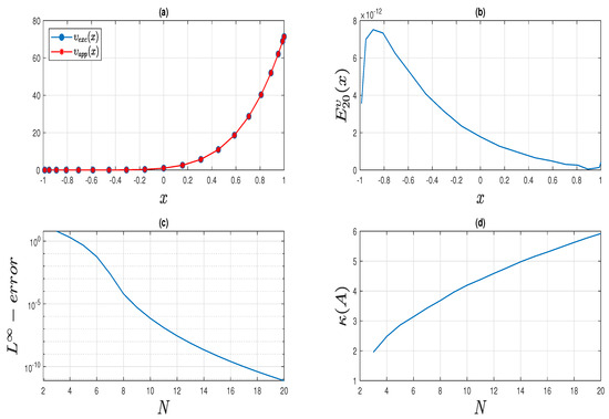
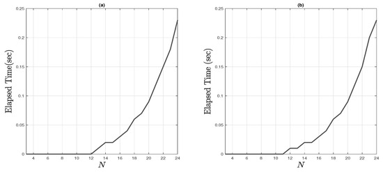
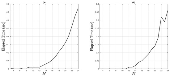
The numerical results are reported in Figure 1, showing excellent approximations using relatively small values of N. And, the elapsed time taken to construct the collocation matrix and the right-hand side vector , as well as the resulting solved linear system (59), are exhibited on the left plot of Figure 2.
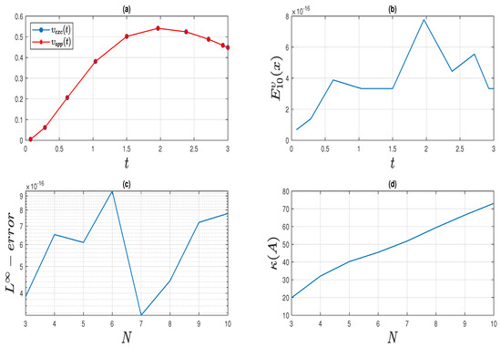
Figure 1.
The numerical results of Example 1 using the PCTFM for with the fractional order and tempering parameter . Plot (a) shows the exact and approximate solutions for . Plot (b) shows the absolute error. Plot (c) shows the norm infinity error for . Plot (d) shows the corresponding condition number .
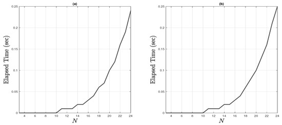
Figure 2.
The elapsed times were taken by the PCTFM to construct the collocation matrices and the vectors and then solve the resulted linear systems of Examples 1 and 2, respectively, against various sizes N. Plot (a) uses , and . Plot (b) uses , and .
Example 2.
Consider the following TFDE:
where the Caputo TFD for , subject to initial condition and
The exact solution to this problem is
To avoid the ill-conditioning of integer differential operators and the reduction in convergence rate for the derivative in the first term, an alternative direction to this example is to recast the TFDE into its integral formulation to take advantage of the well conditioning of integral operators. Thus, apply the first integration of Equation (60), impose the given initial condition, and then use the CPTIM and CPTFDIM to obtain
where denotes the identity matrix of size , is the GL points vector,
and
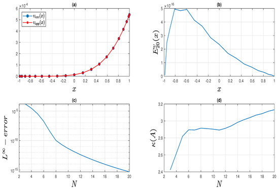
The numerical results are reported in Figure 3. And, the elapsed time taken to construct the collocation matrix and the vector , as well as the resulting linear system (62), are exhibited on the right plot of Figure 2. The non-tempering case of Example 2 was previously solved by two methods in the study by Gholami et al. [54].
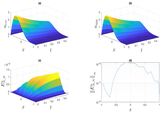
Figure 3.
The numerical results of Example 2 using the PCTFM with the fractional order , and tempering parameter for . Plot (a) shows the exact and approximate solutions for . Plot (b) shows the absolute error. Plot (c) shows the norm infinity error for . Plot (d) shows the corresponding condition number .
Example 3.

Consider the nonlinear TFDE
where
and
for subject to the initial condition , whose analytical solution is given by . This problem was treated before in [12,55]. Using the shifted CPTFDIM at the shifted GL points, we obtain the linear system
where
The numerical results, which include the exact and approximate solutions, the absolute error, and the condition number , are reported in Figure 4 for , , and . The elapsed time taken to evaluate the collocation matrix and the vector , as well as the resulting solved linear system (64), are exhibited on the left plot of Figure 5. Table 1 shows the - and -errors of the numerical solutions using and for . The -error comparison with the method of Morgado and Rebelo [55] at different values of λ and N for and is shown in Table 2.
Figure 4.
The numerical simulation of Example 3 using the PCTFM with the fractional order and tempering parameter for . Plot (a) exhibits the exact and approximate solutions for . Plot (b) shows the absolute error. Plot (c) shows the norm infinity error for . Plot (d) shows the corresponding condition number .
Figure 5.
The elapsed times were taken by the PCTFM to construct the collocation matrices and the vectors and then solve the resulted linear systems of Examples 3 and 4, respectively, against various sizes N. Plot (a) uses , and . Plot (b) uses , and .
Table 1.
The - and -errors of the numerical treatments of Example 3 using the PCTFM for and different small values of N.
Table 2.
A comparison of the -error of Example 3 between the numerical method Morgado and Rebelo [55] and the PCTFM with several values of N and step size with tempering parameter using the fractional orders and .
Example 4.
We consider the following TFDE in the long time interval:
with
and the initial condition for . The exact solution of this initial value problem is . This problem was treated before in [56].
Applying the same steps as previous problems, we have the following algebraic system:
where
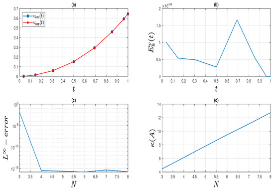
The numerical results, which include the exact and approximate solutions, the absolute error, and the condition number , are reported in Figure 6 for , , and . The elapsed time taken to construct the collocation matrix and the vector , as well as the resulting solved algebraic system (66), are exhibited on the right plot of Figure 5. Table 3 manifests again the superior accuracy of the PCTFM via the - and -errors of the numerical solutions using and for . The -error comparison with the method of Saedshoar Heris and Javidi [56] at different values of N for and is shown in Table 4.
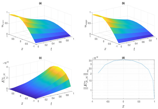
Figure 6.
The numerical simulations of Example 4 using the PCTFM with the fractional order and tempering parameter for . Plot (a) shows the exact and approximate solutions for . Plot (b) shows the absolute error. Plot (c) shows the norm infinity error for . Plot (d) shows the corresponding condition number .
Table 3.
The - and -errors of the numerical treatments of Example 4 using the PCTFM for using different small values of N.
Table 4.
A comparison of the absolute error of Example 4 between the predictor-corrector numerical method of Saedshoar Heris and Javidi [56] and the PCTFM for several values of N versus h with tempering parameter using the fractional orders at .
Example 5.
Consider the time–space-tempered fractional advection–diffusion problem:
with the initial condition together with the boundaries , associated with the fractional orders , and tempering parameters α. A non-tempering case of this problem was discussed before in [57].
Applying the CPTFDIM at the GL points for spatial terms and the shifted CPTFDIM at the shifted GL points for the temporal term, we obtain the linear Lyapunov system
where υ and represent the numerical solution and load matrices whose elements are and , respectively. The exact solution is given by
The left-hand side bi-variant function can be obtained using via Equation (67).
The numerical results, which include the exact and approximate solutions, the absolute error surface, and the norm infinity error for , are reported in Figure 7 for , , and . A cross-section of the exact and approximate solutions is shown at many values of the collocation temporal points t in Figure 8 for , , and tempering parameter using the PCTFM. The elapsed time taken to construct the collocation matrices and the vector , as well as the solved linear Lyapunov system (68), are exhibited on the left plot of Figure 9. Table 5 manifests again the superior accuracy of the PCTFM via the - and -errors of the numerical solutions using , and , for .
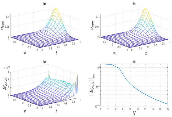
Figure 7.
The numerical simulations of Example 5 using the PCTFM with the fractional orders , and tempering parameter and . Plots (a,b) show the exact and approximate solutions, respectively, for . The plot (c) shows the absolute error. Plot (d) shows the norm infinity error for .
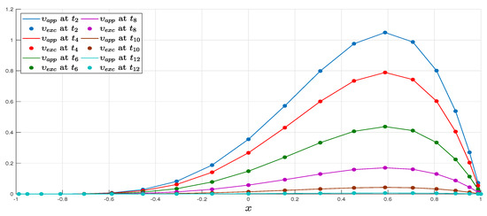
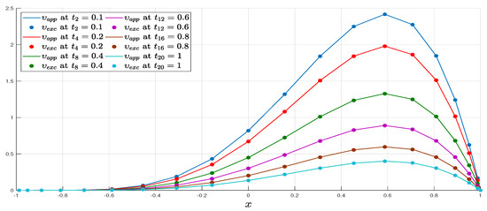
Figure 8.
The exact and approximate solutions of Example 5 using the PCTFM with the fractional orders and tempering parameter for at the collocation points .
Figure 9.
The elapsed times were taken by the PCTFM to perform Examples 5 and 6, respectively, against various sizes N. Plot (a) shows the construction of the collocation matrices and , and the vector , and then the solving of the Lyapunov system Equation (68) with , and . Plot (b) shows the elapsed time taken to confirm the first discretization (70) for using , and .
Table 5.
The - and -errors of the numerical treatments of Example 5 using the PCTFM when , for different values of t and .
Example 6.
One of the most significant advantages of the PCTFM is the efficient numerical treatment of nonlinear tempered fractional differential terms in TFDEs. We consider the nonlinear time-dependent space-tempered fractional Burgers’ equation:
with the initial condition , together with the boundaries , where and . The spatial discretization style can be similarly carried out as shown in previous examples; hence, we have a system of first-order differential equations in the form
where are the components of the solution vector. We perform the time discretization of the resulting system using a Runge–Kutta algorithm of order four (RK-4). We have studied four different values of ν: the inviscid TFBE when , the viscous TFBE with very small diffusivity for , the viscous TFBE with small diffusivity for , and the viscous TFBE with comparatively larger diffusivity for . For each case, the exact solution of such a problem is with the corresponding forcing term
where .
The numerical results, which include the exact and approximate solutions, the absolute error surface, and the norm infinity error for , are reported in Figure 10 for , , and . We employ in our RK-4 multistage time-discretization algorithm. A cross-section of the exact and approximate solutions is shown at many values of the collocation temporal points t in Figure 11 for , and tempering parameter using . The elapsed time taken to perform the first discretization is shown in Equation (70) exhibited on the right plot of Figure 9. Table 6 again manifests the superior accuracy of the PCTFM via the - and -errors of the numerical solutions using , and for .
Figure 10.
The numerical simulation of Example 6 using the PCTFM. Plot (a) exhibits the exact solution on . Plot (b) shows the numerical solution for the same region obtained using . Plot (c) shows the absolute error surface. Plot (d) shows versus x for the parameters and .
Figure 11.
The exact and approximate solutions of Example 6 using the PCTFM for , , for the fractional orders , and tempering parameter at the collocation points .
Table 6.
The - and -errors of the numerical treatments of Example 6 using the PCTFM when , and many values of and x.
Example 7.
Finally, we consider a simple model of the tempered fractional unsteady conjugate heat transfer problem:
with the initial condition , where , and k is a real constant. The spatial discretization style can be similarly carried out as shown in previous examples; hence, we have a system of first-order differential equations in the form
where are the components of the solution vector. We perform the time discretization of the resulting system using a Runge–Kutta algorithm of order four (RK-4). The exact solution of such a problem is .
The numerical results, which include the exact and approximate solutions, the absolute error surface, and the norm infinity error for , are reported in Figure 12 for , , and . We employ in our RK-4 multistage time-discretization algorithm.
Figure 12.
The numerical simulation of Example 7 using the PCTFM. Plot (a) exhibits the exact solution on . Plot (b) shows the numerical solution for the same region obtained using . Plot (c) shows the absolute error surface. Plot (d) shows versus x for the parameters , and .
7. Conclusions
We introduced the development of Chebyshev-tempered fractional pseudospectral operational matrices and their applications. These matrices are constructed using Chebyshev interpolating polynomials at Gauss–Lobatto points, based on the definitions of tempered fractional operators. The key features of the CPTFDIM include a high accuracy in numerical tempered integrations of any order, applicability, and efficiency in finding numerical solutions to TFDEs. We demonstrate that the developed matrix accurately handles any non-integer negative order in the CPTFDIM. Due to the lower computational complexity of the approach, it provides fast and straightforward computation. Numerical results, stability, and convergence analyses show that the error in approximating a function decreases exponentially with an increase in the number of collocation points. Overall, the CPTFDIM offers efficient and rapid convergence rates for numerical computations. Furthermore, our numerical simulations indicate that the condition number of the resulting collocation matrices, denoted as , scales approximately linearly with N. The presented operational matrices are demonstrated to be highly efficient and accurate in dealing with linear and nonlinear problems, surpassing some recently presented techniques in the literature.
As a future aim, we expect to use these matrices to treat an efficient ADI difference scheme for the non-local evolution problem in three-dimensional space, multi-dimensional variable-order tempered fractional Schrödinger equations, and some elliptic problems.
Author Contributions
Conceptualization, T.A.; Software, S.A.D.; Writing—original draft, S.A.D.; Writing—review & editing, A.E.-A.; Visualization, S.A.D. and A.F.; Supervision, H.M.E.-H.; Funding acquisition, A.E.-A. and A.F. All authors have read and agreed to the published version of the manuscript.
Funding
This research received no external funding.
Data Availability Statement
Not applicable.
Acknowledgments
We thank the three anonymous reviewers for their careful reading of the manuscript and their constructive comments and suggestions. The first author extends their appreciation to the Deputyship for Research and Innovation, Ministry of Education in Saudi Arabia for funding this research work through project number: 445-9-397.
Conflicts of Interest
The authors declare no competing interest.
Appendix A. Computational Algorithm
This section presents the simple pseudocode performance of an algorithm that can effectively address Problem 6 using PCTFM. The approximate solution of Problem 6 is computed on a predetermined set of Gauss–Chebyshev nodes via the tempered differential matrices and as a spatial discretization, while the temporal discretization is performed using a direct Runge–Kutta algorithm of order four. The following pseudocode has demonstrated remarkable effectiveness and efficiency in tackling the given problem. Users should be able to utilize the algorithms after reading their descriptions.
| Algorithm A1 PCTFM algorithm for solving tempered fractional Burgers’ problem. |
|
References
- Hendy, A.S.; Zaky, M.A. Combined Galerkin spectral/finite difference method over graded meshes for the generalized nonlinear fractional Schrödinger equation. Nonlinear Dyn. 2021, 103, 2493–2507. [Google Scholar] [CrossRef]
- Roy, R.; Akbar, M.A.; Wazwaz, A.M. Exact wave solutions for the nonlinear time fractional Sharma–Tasso–Olver equation and the fractional Klein–Gordon equation in mathematical physics. Opt. Quantum Electron. 2018, 50, 1–19. [Google Scholar] [CrossRef]
- Podlubny, I. Fractional differential equations. Math. Sci. Eng. 1999, 198, 41–119. [Google Scholar]
- Sabzikar, F.; Meerschaert, M.M.; Chen, J. Tempered fractional calculus. J. Comput. Phys. 2015, 293, 14–28. [Google Scholar] [CrossRef] [PubMed]
- Rosenau, P. Tempered diffusion: A transport process with propagating fronts and inertial delay. Phys. Rev. A 1992, 46, R7371. [Google Scholar] [CrossRef] [PubMed]
- Meerschaert, M.M.; Zhang, Y.; Baeumer, B. Tempered anomalous diffusion in heterogeneous systems. Geophys. Res. Lett. 2008, 35, L17403. [Google Scholar] [CrossRef]
- He, J.Q.; Dong, Y.; Li, S.T.; Liu, H.L.; Yu, Y.J.; Jin, G.Y.; Liu, L.D. Study on force distribution of the tempered glass based on laser interference technology. Optik 2015, 126, 5276–5279. [Google Scholar] [CrossRef]
- Samiee, M.; Akhavan-Safaei, A.; Zayernouri, M. Tempered fractional LES modeling. J. Fluid Mech. 2022, 932, A4. [Google Scholar] [CrossRef]
- Cartea, A.; del Castillo-Negrete, D. Fractional diffusion models of option prices in markets with jumps. Phys. A Stat. Mech. Its Appl. 2007, 374, 749–763. [Google Scholar] [CrossRef]
- Meerschaert, M.M.; Sabzikar, F.; Phanikumar, M.S.; Zeleke, A. Tempered fractional time series model for turbulence in geophysical flows. J. Stat. Mech. Theory Exp. 2014, 2014, P09023. [Google Scholar] [CrossRef]
- Hanyga, A. Wave propagation in media with singular memory. Math. Comput. Model. 2001, 34, 1399–1421. [Google Scholar] [CrossRef]
- Shiri, B.; Wu, G.C.; Baleanu, D. Collocation methods for terminal value problems of tempered fractional differential equations. Appl. Numer. Math. 2020, 156, 385–395. [Google Scholar] [CrossRef]
- Boniece, B.C.; Didier, G.; Sabzikar, F. On fractional Lévy processes: Tempering, sample path properties and stochastic integration. J. Stat. Phys. 2020, 178, 954–985. [Google Scholar] [CrossRef]
- Aboelenen, T. Stability analysis and error estimates of implicit–explicit Runge–Kutta local discontinuous Galerkin methods for nonlinear fractional convection–diffusion problems. Comput. Appl. Math. 2022, 41, 1–27. [Google Scholar] [CrossRef]
- Carr, P.; Geman, H.; Madan, D.B.; Yor, M. Stochastic volatility for Lévy processes. Math. Financ. 2003, 13, 345–382. [Google Scholar] [CrossRef]
- Zhang, Y.; Meerschaert, M.M.; Packman, A.I. Linking fluvial bed sediment transport across scales. Geophys. Res. Lett. 2012, 39, L20404. [Google Scholar] [CrossRef]
- Meerschaert, M.M.; Sabzikar, F. Tempered fractional Brownian motion. Stat. Probab. Lett. 2013, 83, 2269–2275. [Google Scholar] [CrossRef]
- Cao, J.; Li, C.; Chen, Y. On tempered and substantial fractional calculus. In Proceedings of the 2014 IEEE/ASME 10th International Conference on Mechatronic and Embedded Systems and Applications (MESA), Senigallia, Italy, 10–12 September 2014; IEEE: Piscataway, NJ, USA, 2014; pp. 1–6. [Google Scholar]
- Ding, H.; Li, C. A high-order algorithm for time-Caputo-tempered partial differential equation with Riesz derivatives in two spatial dimensions. J. Sci. Comput. 2019, 80, 81–109. [Google Scholar] [CrossRef]
- Zhao, L.; Deng, W.; Hesthaven, J.S. Spectral methods for tempered fractional differential equations. Math. Comput. 2016. [Google Scholar]
- Deng, J.; Zhao, L.; Wu, Y. Fast predictor-corrector approach for the tempered fractional differential equations. Numer. Algorithms 2017, 74, 717–754. [Google Scholar] [CrossRef]
- Alrawashdeh, M.S.; Kelly, J.F.; Meerschaert, M.M.; Scheffler, H.P. Applications of inverse tempered stable subordinators. Comput. Math. Appl. 2017, 73, 892–905. [Google Scholar] [CrossRef]
- Lu, B.; Zhang, Y.; Reeves, D.M.; Sun, H.; Zheng, C. Application of tempered-stable time fractional-derivative model to upscale subdiffusion for pollutant transport in field-scale discrete fracture networks. Mathematics 2018, 6, 5. [Google Scholar] [CrossRef]
- Rawashdeh, M.S. The fractional natural decomposition method: Theories and applications. Math. Methods Appl. Sci. 2017, 40, 2362–2376. [Google Scholar] [CrossRef]
- Rawashdeh, M.S.; Al-Jammal, H. Numerical solutions for systems of nonlinear fractional ordinary differential equations using the FNDM. Mediterr. J. Math. 2016, 13, 4661–4677. [Google Scholar] [CrossRef]
- Rawashdeh, M.S. An efficient approach for time-fractional damped Burger and time-Sharma-Tasso-Olver equations using the FRDTM. Appl. Math. Inf. Sci. 2015, 9, 1239. [Google Scholar]
- Sejdić, E.; Djurović, I.; Stanković, L. Fractional Fourier transform as a signal processing tool: An overview of recent developments. Signal Process. 2011, 91, 1351–1369. [Google Scholar] [CrossRef]
- Obeidat, N.A.; Bentil, D.E. New theories and applications of tempered fractional differential equations. Nonlinear Dyn. 2021, 105, 1689–1702. [Google Scholar] [CrossRef]
- Zhao, W.; Maitama, S. Beyond Sumudu transform and natural transform: J-transform properties and applications. J. Appl. Anal. Comput. 2020, 10, 1223–1241. [Google Scholar]
- Grandclément, P.; Fodor, G.; Forgács, P. Numerical simulation of oscillatons: Extracting the radiating tail. Phys. Rev. D 2011, 84, 065037. [Google Scholar] [CrossRef]
- Guo, B. Some progress in spectral methods. Sci. China Math. 2013, 56, 2411–2438. [Google Scholar] [CrossRef]
- Bhrawy, A.H.; Alofi, A.S. A Jacobi–Gauss collocation method for solving nonlinear Lane–Emden type equations. Commun. Nonlinear Sci. Numer. Simul. 2012, 17, 62–70. [Google Scholar] [CrossRef]
- Burns, K.J.; Vasil, G.M.; Oishi, J.S.; Lecoanet, D.; Brown, B.P. Dedalus: A flexible framework for numerical simulations with spectral methods. Phys. Rev. Res. 2020, 2, 023068. [Google Scholar] [CrossRef]
- Miquel, B.; Julien, K. Hybrid Chebyshev function bases for sparse spectral methods in parity-mixed PDEs on an infinite domain. J. Comput. Phys. 2017, 349, 474–500. [Google Scholar] [CrossRef]
- Viswanath, D. Spectral integration of linear boundary value problems. J. Comput. Appl. Math. 2015, 290, 159–173. [Google Scholar] [CrossRef]
- Doha, E.H.; Bhrawy, A.H.; Baleanu, D.; Ezz-Eldien, S.S. On shifted Jacobi spectral approximations for solving fractional differential equations. Appl. Math. Comput. 2013, 219, 8042–8056. [Google Scholar] [CrossRef]
- Bhrawy, A.H.; Ezz-Eldien, S.S.; Doha, E.H.; Abdelkawy, M.A.; Baleanu, D. Solving fractional optimal control problems within a Chebyshev–Legendre operational technique. Int. J. Control 2017, 90, 1230–1244. [Google Scholar] [CrossRef]
- Zaky, M.; Ezz-Eldien, S.; Doha, E.; Tenreiro Machado, J.; Bhrawy, A. An efficient operational matrix technique for multidimensional variable-order time fractional diffusion equations. J. Comput. Nonlinear Dyn. 2016, 11, 061002. [Google Scholar] [CrossRef]
- Dabiri, A.; Butcher, E.A. Efficient modified Chebyshev differentiation matrices for fractional differential equations. Commun. Nonlinear Sci. Numer. Simul. 2017, 50, 284–310. [Google Scholar] [CrossRef]
- Dahy, S.A.; Elgindy, K.T. High-order numerical solution of viscous Burgers’ equation using an extended Cole–Hopf barycentric Gegenbauer integral pseudospectral method. Int. J. Comput. Math. 2022, 99, 446–464. [Google Scholar] [CrossRef]
- Elgindy, K.T.; Dahy, S.A. High-order numerical solution of viscous Burgers’ equation using a Cole-Hopf barycentric Gegenbauer integral pseudospectral method. Math. Methods Appl. Sci. 2018, 41, 6226–6251. [Google Scholar] [CrossRef]
- Moghaddam, B.P.; Machado, J.; Babaei, A. A computationally efficient method for tempered fractional differential equations with application. Comput. Appl. Math. 2018, 37, 3657–3671. [Google Scholar] [CrossRef]
- Bhrawy, A.; Zaky, M. Numerical simulation for two-dimensional variable-order fractional nonlinear cable equation. Nonlinear Dyn. 2015, 80, 101–116. [Google Scholar] [CrossRef]
- Dabiri, A.; Butcher, E.A.; Nazari, M. Coefficient of restitution in fractional viscoelastic compliant impacts using fractional Chebyshev collocation. J. Sound Vib. 2017, 388, 230–244. [Google Scholar] [CrossRef]
- Dabiri, A.; Nazari, M.; Butcher, E.A. Optimal fractional state feedback control for linear fractional periodic time-delayed systems. In Proceedings of the 2016 American Control Conference (ACC), Boston, MA, USA, 6–8 July 2016; IEEE: Piscataway, NJ, USA, 2016; pp. 2778–2783. [Google Scholar]
- Stenger, F. Handbook of Sinc Numerical Methods; CRC Press: Boca Raton, FL, USA, 2016. [Google Scholar]
- Piessens, R. Computing integral transforms and solving integral equations using Chebyshev polynomial approximations. J. Comput. Appl. Math. 2000, 121, 113–124. [Google Scholar] [CrossRef]
- Huang, Z.; Boyd, J.P. Bandwidth truncation for Chebyshev polynomial and ultraspherical/Chebyshev Galerkin discretizations of differential equations: Restrictions and two improvements. J. Comput. Appl. Math. 2016, 302, 340–355. [Google Scholar] [CrossRef]
- Boyd, J.P. Large-degree asymptotics and exponential asymptotics for Fourier, Chebyshev and Hermite coefficients and Fourier transforms. J. Eng. Math. 2009, 63, 355–399. [Google Scholar] [CrossRef]
- Gutleb, T.; Carrillo, J.; Olver, S. Computing equilibrium measures with power law kernels. Math. Comput. 2022, 91, 2247–2281. [Google Scholar] [CrossRef]
- Bulychev, Y.G.; Bulycheva, E.Y. Some new properties of the Chebyshev polynomials and their use in analysis and design of dynamic systems. Autom. Remote Control 2003, 64, 554–563. [Google Scholar] [CrossRef]
- Elbarbary, E.M.; El-Sayed, S.M. Higher order pseudospectral differentiation matrices. Appl. Numer. Math. 2005, 55, 425–438. [Google Scholar] [CrossRef]
- Elbarbary, E.M. Pseudospectral integration matrix and boundary value problems. Int. J. Comput. Math. 2007, 84, 1851–1861. [Google Scholar] [CrossRef]
- Gholami, S.; Babolian, E.; Javidi, M. Fractional pseudospectral integration/differentiation matrix and fractional differential equations. Appl. Math. Comput. 2019, 343, 314–327. [Google Scholar] [CrossRef]
- Morgado, M.L.; Rebelo, M. Well-posedness and numerical approximation of tempered fractional terminal value problems. Fract. Calc. Appl. Anal. 2017, 20, 1239–1262. [Google Scholar] [CrossRef][Green Version]
- Saedshoar Heris, M.; Javidi, M. A predictor–corrector scheme for the tempered fractional differential equations with uniform and non-uniform meshes. J. Supercomput. 2019, 75, 8168–8206. [Google Scholar] [CrossRef]
- Zayernouri, M.; Karniadakis, G.E. Fractional spectral collocation method. SIAM J. Sci. Comput. 2014, 36, A40–A62. [Google Scholar] [CrossRef]


Disclaimer/Publisher’s Note: The statements, opinions and data contained in all publications are solely those of the individual author(s) and contributor(s) and not of MDPI and/or the editor(s). MDPI and/or the editor(s) disclaim responsibility for any injury to people or property resulting from any ideas, methods, instructions or products referred to in the content. |
© 2023 by the authors. Licensee MDPI, Basel, Switzerland. This article is an open access article distributed under the terms and conditions of the Creative Commons Attribution (CC BY) license (https://creativecommons.org/licenses/by/4.0/).