Multiple Terms Identification of Time Fractional Diffusion Equation with Symmetric Potential from Nonlocal Observation

Abstract

This paper considers a simultaneous identification problem of a time-fractional diffusion equation with a symmetric potential, which aims to identify the fractional order, the potential function, and the Robin coefficient from a nonlocal observation. Firstly, the existence and uniqueness of the weak solution are established for the forward problem. Then, by the asymptotic behavior of the Mittag-Leffler function, the Laplace transform, and the analytic continuation theory, the uniqueness of the simultaneous identification problem is proved under some appropriate assumptions. Finally, the Levenberg–Marquardt method is employed to solve the simultaneous identification problem for finding stably approximate solutions of the fractional order, the potential function, and the Robin coefficient. Numerical experiments for three test cases are given to demonstrate the effectiveness of the presented inversion method.

1. Introduction

With deepening research on inverse problems of fractional-order differential equations, many scholars have focused on parameters’ inversions of time-fractional diffusion equations and achieved a series of significant research results. For single-parameter inverse problems of time-fractional diffusion equations, the authors in [1,2,3] studied the identification problems of the source terms in the control equations. In [4], the contraction and monotonicity-based reconstruction operator was introduced to recover a spatial potential function from the terminal data. The works in [5,6] studied the identification problems of Robin coefficients in the boundary conditions. For the time-fractional diffusion-wave equations, the authors in [7] applied the Levenberg–Marquardt regularization method to identify a time-dependent zeroth-order coefficient and proved the conditional stability of the identification problem; the authors in [8] proved the existence and uniqueness of identifying a spatial-dependent zeroth-order coefficient by using the data measured at a boundary point; the authors in [9] proposed a generalized quasi-boundary value regularization method to identify the spatially related source term from the final time measurements.

Recently, the multiparameter inverse problems of time-fractional diffusion equations have attracted the attention of many scholars both domestically and internationally. The work in [10] studied the simultaneous recovery of fractional orders and the spatially related source term from the partial Cauchy boundary data. The works in [11,12] employed an alternating minimization algorithm to investigate the simultaneous identification of the source term and fractional orders by using two different types of observation data. In [13], the authors utilized the asymptotic behavior of Mittag-Leffler functions and the Marchenko uniqueness theorem to study the simultaneous inverse problem of identifying the fractional order, the spatial potential, and the Robin coefficients under nonuniform boundary conditions. The works in [14,15] applied the Levenberg–Marquardt regularization method and the conjugate gradient method, respectively, to simultaneously recover the spatial potential and the fractional order from the Cauchy data. Both studies established the uniqueness of the simultaneous inversion problem by using Laplace transform and Gel’fand–Levitan theory. In [16,17], the Levenberg–Marquardt regularization method was utilized to reconstruct the temporal potential term in a multi-term time-fractional diffusion equation. The work in [18] investigated the inverse problem of recovering the spatial potential term and the fractional order from the transversal Cauchy data without assuming full knowledge of the initial data and source term, where the authors proposed a two-stage numerical identification method for reconstructing the fractional order and the potential coefficient. For the time-fractional diffusion-wave equation, the authors in [19] studied the nonlinear inverse problem of identifying the fractional orders and the temporal potential term from the integral data. They proved the uniqueness of the simultaneous inversion problem and presented a Bayesian method for numerically reconstructing the temporal potential and the fractional orders. In [20], the authors proposed a nonstationary iterative Tikhonov regularization to simultaneously identify the time-dependent potential coefficient and the temporal source term from two-point observation data. In [21], the authors studied the inverse problem of identifying the zeroth-order coefficient and the fractional order simultaneously in a time-fractional reaction-diffusion-wave equation and obtained the uniqueness of the simultaneously inverse problem.

In this paper, we consider the following problem of the time-fractional diffusion equation:

$$\left\{\begin{array}{cc}{\mathsf{\partial }}_t^{\mathit{\alpha }}u(x,t)={\displaystyle \frac{{\mathsf{\partial }}^{2}u(x,t)}{\mathsf{\partial }{x}^2}}-q\left(x\right)u(x,t),\hfill & \hfill (x,t)\in (0,1)\times (0,T],\\ u(x,0)=0,\hfill & \hfill x\in [0,1],\\ \frac{\mathsf{\partial }u(0,t)}{\mathsf{\partial }x}-\mathit{\kappa }u(0,t)=0,\hfill & \hfill t\in (0,T],\\ \frac{\mathsf{\partial }u(1,t)}{\mathsf{\partial }x}+\mathit{\kappa }u(1,t)=\mathit{\mu }\left(t\right),\hfill & \hfill t\in (0,T],\end{array}\right.$$

(1)

where $q\left(x\right)\ge 0$ is a symmetric potential due to $q\left(x\right)=q(1-x),x\in [0,1]$ and ${\mathsf{\partial }}_t^{\mathit{\alpha }}u(x,t)$ is the $\mathit{\alpha }$ order Caputo fractional derivative of the time variable t, and it is defined as

$${\mathsf{\partial }}_t^{\mathit{\alpha }}u(x,t)=\frac{1}{\Gamma (1-\mathit{\alpha })}{\int }_0^t\frac{\mathsf{\partial }u(x,s)}{\mathsf{\partial }s}\frac{\mathrm{d}s}{{(t-s)}^{\mathit{\alpha }}},\mathit{\alpha }\in (0,1).$$

(2)

If the potential function $q\left(x\right)$, the Robin coefficient $\mathit{\kappa }$, and the boundary condition $\mathit{\mu }\left(t\right)$ in problem (1) are known, finding the distribution of the physical quantity u is called the direct problem. However, our focus here is on the inverse problem of determining simultaneously the potential function $q\left(x\right)$, the Robin coefficient $\mathit{\kappa }$, and the fractional order $\mathit{\alpha }$ in problem (1) from the known boundary value $\mathit{\mu }\left(t\right)$ and the following nonlocal condition:

$$d\left(t\right)={\int }_0^1\mathit{\omega }\left(x\right)u(x,t)\mathrm{d}x,0<t\le T,$$

(3)

where $\mathit{\omega }\left(x\right)\in L^2[0,1]$ is the weight function.

The remainder of this paper is organized as follows. Some preliminary knowledge and the solution of the direct problem are presented in Section 2. Then, the uniqueness of the simultaneous inversion problem is stated in Section 3, and it is proved by the use of the asymptotic behavior of the Mittag-Leffler function, the Laplace transform, and the analytic continuation theory. In Section 4, a numerical algorithm based on the Levenberg–Marquardt method is provided for solving the simultaneous inversion problem. Several numerical experiments are given in Section 5 to demonstrate the effectiveness of simultaneously identifying the fractional order, potential function, and Robin coefficient. Finally, Section 6 summarizes this paper.

2. Preliminary and Weak Solution of the Direct Problem

In this section, we give some preliminaries, such as the definition and propositions of the two-parameter Mittag-Leffler function, and present the weak solution to direct problem (1).

2.1. Preliminary

Definition 1. 

The two-parameter Mittag-Leffler function is defined by

$$E_{\mathit{\alpha },\mathit{\beta }}\left(z\right)=\sum _{k=0}^{\infty }\frac{z^k}{\Gamma (\mathit{\alpha }k+\mathit{\beta })},z\in \mathbb{C},$$

where $\mathit{\alpha }>0$, $\mathit{\beta }>0$ are two positive constants.

Proposition 1. 

Let $0<\mathit{\alpha }<1$ and $\mathit{\lambda }>0$, and then we have

$$\begin{array}{cc}\hfill & \frac{\mathrm{d}}{\mathrm{d}t}{E}_{\mathit{\alpha },1}(-\mathit{\lambda }{t}^{\mathit{\alpha }})=-\mathit{\lambda }{t}^{\mathit{\alpha }-1}{E}_{\mathit{\alpha },\mathit{\alpha }}(-\mathit{\lambda }{t}^{\mathit{\alpha }}),t>0.\hfill \end{array}$$

(4)

Proposition 2. 

Let $0<\mathit{\alpha }<2$ and $\mathit{\beta }\in \mathbb{R}$. Suppose that ς satisfies ${\displaystyle \frac{\mathit{\pi }\mathit{\alpha }}{2}}<\mathit{\varsigma }<min\{\mathit{\pi },\mathit{\pi }\mathit{\alpha }\}$. Then, there exists a constant $c=c(\mathit{\alpha },\mathit{\beta },\mathit{\varsigma })>0$ such that

$$\left|E_{\mathit{\alpha },\mathit{\beta }}\left(z\right)\right|\le \frac{c}{1+\left|z\right|},\mathit{\varsigma }\le |arg\left(z\right)|\le \mathit{\pi }.$$

(5)

Lemma 1 

([6,18]). Let $0<\mathit{\alpha }<1$ and $\mathit{\lambda }>0$. If $\mathit{\mu }\left(t\right)\in AC[0,T]$, we have

$$\begin{array}{cc}\hfill & {\mathsf{\partial }}_t^{\mathit{\alpha }}{\int }_0^t\mathit{\mu }(\mathit{\tau }){(t-\mathit{\tau })}^{\mathit{\alpha }-1}{E}_{\mathit{\alpha },\mathit{\alpha }}(-\mathit{\lambda }{(t-\mathit{\tau })}^{\mathit{\alpha }})\mathrm{d}\mathit{\tau }\hfill \\ \hfill & =\mathit{\mu }\left(t\right)-\mathit{\lambda }{\int }_0^t\mathit{\mu }(\mathit{\tau }){(t-\mathit{\tau })}^{\mathit{\alpha }-1}{E}_{\mathit{\alpha },\mathit{\alpha }}(-\mathit{\lambda }{(t-\mathit{\tau })}^{\mathit{\alpha }})\mathrm{d}\mathit{\tau },0<t\le T.\hfill \end{array}$$

(6)

Moreover, if $\mathit{\mu }\left(t\right)\in C^1[0,1]$, we have

$$\begin{array}{cc}\hfill & {\int }_0^t{(t-\mathit{\tau })}^{\mathit{\alpha }-1}{E}_{\mathit{\alpha },\mathit{\alpha }}(-\mathit{\lambda }{(t-\mathit{\tau })}^{\mathit{\alpha }}){\mathsf{\partial }}_{\mathit{\tau }}^{\mathit{\alpha }}\mathit{\mu }(\mathit{\tau })\mathrm{d}\mathit{\tau }\hfill \\ \hfill & =\mathit{\mu }\left(t\right)-\mathit{\mu }\left(0\right)E_{\mathit{\alpha },1}(-\mathit{\lambda }{t}^{\mathit{\alpha }})-\mathit{\lambda }{\int }_0^t\mathit{\mu }(\mathit{\tau }){(t-\mathit{\tau })}^{\mathit{\alpha }-1}{E}_{\mathit{\alpha },\mathit{\alpha }}(-\mathit{\lambda }{(t-\mathit{\tau })}^{\mathit{\alpha }})\mathrm{d}\mathit{\tau }.\hfill \end{array}$$

(7)

Lemma 2. 

([22]). (Convolution Young inequality). Suppose that $f\in L^p\left({\mathbb{R}}^d\right)$, $g\in L^q\left({\mathbb{R}}^d\right)$ for $1\le p,q,r\le \infty$, and

$${\displaystyle \frac{1}{p}}+{\displaystyle \frac{1}{q}}={\displaystyle \frac{1}{r}}+1.$$

Then, we have ${\parallel f\ast g\parallel }_r\le {\parallel f\parallel }_p{\parallel g\parallel }_q$, where the symbol ∗ represents the convolution of two functions.

Define the differential operator $\mathcal{A}$ by

$$\mathcal{A}u(x,t)=-{\displaystyle \frac{{\mathsf{\partial }}^{2}u(x,t)}{\mathsf{\partial }{x}^2}}+q\left(x\right)u(x,t),$$

(8)

and let $\{{\mathit{\lambda }}_n,{\mathit{\varphi }}_n\left(x\right)\}$ satisfy the initial value problem:

$$\left\{\begin{array}{cc}\mathcal{A}{\mathit{\varphi }}_n\left(x\right)={\mathit{\lambda }}_n{\mathit{\varphi }}_n\left(x\right),\hfill & x\in (0,1),\hfill \\ {\mathit{\varphi }}_n\left(0\right)=1,{\mathit{\varphi }}_n^{\prime }\left(0\right)=\mathit{\kappa }.\hfill \end{array}\right.$$

(9)

According to the spectral theory of Sturm–Liouville eigenvalue problems [23], ${\{{\mathit{\lambda }}_n,{\mathit{\varphi }}_n\left(x\right)\}}_{n=1}^{\infty }$ is the eigenpairs of operator $\mathcal{A}$, and it can make it that ${\mathit{\varphi }}_n\left(1\right)=1$ always holds true. Moreover, ${\left\{{\mathit{\lambda }}_n\right\}}_{n=1}^{\infty }$ is a strictly increasing sequence, and ${\left\{{\mathit{\varphi }}_n\left(x\right)\right\}}_{n=1}^{\infty }$ can be chosen to form an orthonormal basis of the space $L^2(0,1)$. Denote ${\mathit{\rho }}_n={\parallel {\mathit{\varphi }}_n\parallel }_{L^2(0,1)}^{-2}$. Then, we have the asymptotic properties ${\mathit{\rho }}_n=c_0+o\left(1\right),{\mathit{\varphi }}_n\left(x\right)=cos((n-1)\mathit{\pi }x)+o\left(1\right)$ and ${\mathit{\lambda }}_n={(n-1)}^2{\mathit{\pi }}^2+O\left(1\right),n\to \infty$ for $\{{\mathit{\lambda }}_n,{\mathit{\varphi }}_n\left(x\right)\}$.

Definition 2. 

For a given $\mathit{\gamma }\in R$, we define a Hilbert space of fractional power ${\mathcal{A}}^{\mathit{\gamma }}$ by

$$D\left({\mathcal{A}}^{\mathit{\gamma }}\right)=\left\{\mathit{\psi }\in L^2(\Omega ):\sum _{n=1}^{\infty }{\mathit{\lambda }}_n^{2\mathit{\gamma }}{\mathit{\rho }}_n{\left|(\mathit{\psi },{\mathit{\varphi }}_n)\right|}^2<\infty \right\},$$

(10)

with the associated norm

$${\parallel \mathit{\psi }\parallel }_{D\left({\mathcal{A}}^{\mathit{\gamma }}\right)}={\left(\sum _{n=1}^{\infty }{\mathit{\lambda }}_n^{2\mathit{\gamma }}{\mathit{\rho }}_n{\left|(\mathit{\psi },{\mathit{\varphi }}_n)\right|}^2\right)}^{\frac{1}{2}},$$

(11)

where $(·,·)$ represents the scalar product in $L^2[0,1]$.

2.2. The Weak Solution of the Direct Problem

Now, we are ready to state and prove the representation formula for the weak solution to direct problem (1).

Definition 3. 

If $u\in L^2(0,T;D\left({\mathcal{A}}^{\mathit{\gamma }}\right))$ satisfies $u(x,0)=0$ for a.e. $x\in [0,1]$, together with ${\mathsf{\partial }}_t^{\mathit{\alpha }}u\in L^2(0,T;D\left({\mathcal{A}}^{\mathit{\gamma }-1}\right))$, and the following weak form holds:

$${({\mathsf{\partial }}_t^{\mathit{\alpha }}u(·,t),\mathit{\varphi })}_{L^2(0,1)}-{(u(·,t),\mathit{\varphi }{}^{\prime \prime })}_{L^2(0,1)}-\mathit{\mu }\left(t\right)\mathit{\varphi }\left(1\right)+{(u(·,t),q\mathit{\varphi })}_{L^2(0,1)}=0,t\in (0,T),$$

(12)

then, u is called a weak solution of direct problem (1).

Theorem 1. 

Let $\mathit{\mu }\left(t\right)\in AC[0,1]\bigcap C^1[0,1]$. Then, direct problem (1) has a unique weak solution of $u(x,t)\in L^2(0,T;D\left({\mathcal{A}}^{\mathit{\gamma }}\right))$, with ${\mathsf{\partial }}_t^{\mathit{\alpha }}u(x,t)\in L^2(0,T;D\left({\mathcal{A}}^{\mathit{\gamma }-1}\right))$, where the unique solution $u(x,t)$ can be expressed as

$$u(x,t)=\sum _{n=1}^{\infty }{\mathit{\rho }}_n{\int }_0^t\mathit{\mu }(\mathit{\tau }){(t-\mathit{\tau })}^{\mathit{\alpha }-1}{E}_{\mathit{\alpha },\mathit{\alpha }}\left(-{\mathit{\lambda }}_n{(t-\mathit{\tau })}^{\mathit{\alpha }}\right)\mathrm{d}\mathit{\tau }{\mathit{\varphi }}_n\left(x\right).$$

(13)

Proof. 

Firstly, we derive Formula (13). Let $v(x,t)=u(x,t)-e\left(x\right)\mathit{\mu }\left(t\right)$ with $e\left(x\right)=$${(\mathit{\kappa }+2)}^{-1}{x}^2$. The direct calculations show that $v(x,t)$ satisfies

$$\left\{\begin{array}{cc}{\mathsf{\partial }}_t^{\mathit{\alpha }}v(x,t)+\mathcal{A}v(x,t)=f(x,t),\hfill & \hfill (x,t)\in (0,1)\times (0,T],\\ v(x,0)=-e\left(x\right)\mathit{\mu }\left(0\right),\hfill & \hfill x\in [0,1],\\ \frac{\mathsf{\partial }v(0,t)}{\mathsf{\partial }x}-\mathit{\kappa }v(0,t)=0,\hfill & \hfill t\in (0,T],\\ \frac{\mathsf{\partial }v(1,t)}{\mathsf{\partial }x}+\mathit{\kappa }v(1,t)=0,\hfill & \hfill t\in (0,T],\end{array}\right.$$

(14)

where $f(x,t)=-e\left(x\right){\mathsf{\partial }}_t^{\mathit{\alpha }}\mathit{\mu }\left(t\right)-\mathcal{A}(e\left(x\right)\mathit{\mu }\left(t\right))$. By the method of the separation of variables in [24], $v(x,t)$ can be expressed by

$$\begin{array}{cc}\hfill v(x,t)& =\sum _{n=1}^{\infty }{\mathit{\rho }}_n{E}_{\mathit{\alpha },1}(-{\mathit{\lambda }}_n{t}^{\mathit{\alpha }})({\mathit{\varphi }}_n,v(x,0)){\mathit{\varphi }}_n\left(x\right)\hfill \\ \hfill & +\sum _{n=1}^{\infty }{\mathit{\rho }}_n{\int }_0^t{(t-\mathit{\tau })}^{\mathit{\alpha }-1}{E}_{\mathit{\alpha },\mathit{\alpha }}(-{\mathit{\lambda }}_n{(t-\mathit{\tau })}^{\mathit{\alpha }})({\mathit{\varphi }}_n,f(x,\mathit{\tau }))\mathrm{d}\mathit{\tau }{\mathit{\varphi }}_n\left(x\right).\hfill \end{array}$$

(15)

By Formula (7), it can be deduced that

$$\begin{array}{cc}\hfill & {\int }_0^t{(t-\mathit{\tau })}^{\mathit{\alpha }-1}{E}_{\mathit{\alpha },\mathit{\alpha }}(-{\mathit{\lambda }}_n{(t-\mathit{\tau })}^{\mathit{\alpha }})({\mathit{\varphi }}_n,f(x,\mathit{\tau }))\mathrm{d}\mathit{\tau }\hfill \\ \hfill & =-{\int }_0^t{(t-\mathit{\tau })}^{\mathit{\alpha }-1}{E}_{\mathit{\alpha },\mathit{\alpha }}(-{\mathit{\lambda }}_n{(t-\mathit{\tau })}^{\mathit{\alpha }})[{\mathsf{\partial }}_{\mathit{\tau }}^{\mathit{\alpha }}\mathit{\mu }(\mathit{\tau })(e,{\mathit{\varphi }}_n)-\mathit{\mu }(\mathit{\tau })(-\mathcal{A}e,{\mathit{\varphi }}_n)]\mathrm{d}\mathit{\tau }\hfill \\ \hfill & =-\left[\mathit{\mu }\left(t\right)-\mathit{\mu }\left(0\right)E_{\mathit{\alpha },1}(-{\mathit{\lambda }}_n{t}^{\mathit{\alpha }})-{\mathit{\lambda }}_n{\int }_0^t{(t-\mathit{\tau })}^{\mathit{\alpha }-1}{E}_{\mathit{\alpha },\mathit{\alpha }}(-{\mathit{\lambda }}_n{(t-\mathit{\tau })}^{\mathit{\alpha }})\mathit{\mu }(\mathit{\tau })\mathrm{d}\mathit{\tau }\right](e,{\mathit{\varphi }}_n)\hfill \\ \hfill & +{\int }_0^t{(t-\mathit{\tau })}^{\mathit{\alpha }-1}{E}_{\mathit{\alpha },\mathit{\alpha }}(-{\mathit{\lambda }}_n{(t-\mathit{\tau })}^{\mathit{\alpha }})\mathit{\mu }(\mathit{\tau })\mathrm{d}\mathit{\tau }(-\mathcal{A}e,{\mathit{\varphi }}_n)\hfill \\ \hfill & =-\left[\mathit{\mu }\left(t\right)-\mathit{\mu }\left(0\right)E_{\mathit{\alpha },1}(-{\mathit{\lambda }}_n{t}^{\mathit{\alpha }})\right](e,{\mathit{\varphi }}_n)\hfill \\ \hfill & +{\int }_0^t{(t-\mathit{\tau })}^{\mathit{\alpha }-1}{E}_{\mathit{\alpha },\mathit{\alpha }}(-{\mathit{\lambda }}_n{(t-\mathit{\tau })}^{\mathit{\alpha }})\mathit{\mu }(\mathit{\tau })\mathrm{d}\mathit{\tau }\left[{\mathit{\lambda }}_n(e,{\mathit{\varphi }}_n)+(-\mathcal{A}e,{\mathit{\varphi }}_n)\right].\hfill \end{array}$$

Noticing that $\{{\mathit{\lambda }}_n,{\mathit{\varphi }}_n\left(x\right)\}$ is the eigensystem of the problem

$$\left\{\begin{array}{cc}\mathcal{A}{\mathit{\varphi }}_n\left(x\right)={\mathit{\lambda }}_n{\mathit{\varphi }}_n\left(x\right),\hfill & x\in (0,1),\hfill \\ {\mathit{\varphi }}_n^{\prime }\left(0\right)-\mathit{\kappa }{\mathit{\varphi }}_n\left(0\right)=0,\hfill \\ {\mathit{\varphi }}_n^{\prime }\left(1\right)+\mathit{\kappa }{\mathit{\varphi }}_n\left(1\right)=0,\hfill \end{array}\right.$$

(16)

by the use of integration by parts, we obtain

$$\begin{array}{cc}\hfill {\mathit{\lambda }}_n(e,{\mathit{\varphi }}_n)+(-\mathcal{A}e,{\mathit{\varphi }}_n)& =(e,\mathcal{A}{\mathit{\varphi }}_n)+(-\mathcal{A}e,{\mathit{\varphi }}_n)\hfill \\ \hfill & =e^{\prime }{\mathit{\varphi }}_n{{|}_{x=0}^{x=1}-e{\mathit{\varphi }}_n^{\prime }|}_{x=0}^{x=1}\hfill \\ \hfill & =e^{\prime }\left(1\right){\mathit{\varphi }}_n\left(1\right)-e^{\prime }\left(0\right){\mathit{\varphi }}_n\left(0\right)-e\left(1\right){\mathit{\varphi }}_n^{\prime }\left(1\right)+e\left(0\right){\mathit{\varphi }}_n^{\prime }\left(0\right)\hfill \\ \hfill & ={\mathit{\varphi }}_n\left(1\right)=1.\hfill \end{array}$$

Therefore, we have

$$\begin{array}{cc}\hfill & {\int }_0^t{(t-\mathit{\tau })}^{\mathit{\alpha }-1}{E}_{\mathit{\alpha },\mathit{\alpha }}(-{\mathit{\lambda }}_n{(t-\mathit{\tau })}^{\mathit{\alpha }})({\mathit{\varphi }}_n,f(x,\mathit{\tau }))\mathrm{d}\mathit{\tau }\hfill \\ \hfill & =-\left[\mathit{\mu }\left(t\right)-\mathit{\mu }\left(0\right)E_{\mathit{\alpha },1}(-{\mathit{\lambda }}_n{t}^{\mathit{\alpha }})\right](e,{\mathit{\varphi }}_n)+{\int }_0^t{(t-\mathit{\tau })}^{\mathit{\alpha }-1}{E}_{\mathit{\alpha },\mathit{\alpha }}(-{\mathit{\lambda }}_n{(t-\mathit{\tau })}^{\mathit{\alpha }})\mathit{\mu }(\mathit{\tau })\mathrm{d}\mathit{\tau }.\hfill \end{array}$$

Thus, $v(x,t)$ is reformulated into

$$v(x,t)=-e\left(x\right)\mathit{\mu }\left(t\right)+\sum _{n=1}^{\infty }{\mathit{\rho }}_n{\int }_0^t{(t-\mathit{\tau })}^{\mathit{\alpha }-1}{E}_{\mathit{\alpha },\mathit{\alpha }}(-{\mathit{\lambda }}_n{(t-\mathit{\tau })}^{\mathit{\alpha }})\mathit{\mu }(\mathit{\tau })\mathrm{d}\mathit{\tau }{\mathit{\varphi }}_n\left(x\right),$$

which implies that

$$u(x,t)=\sum _{n=1}^{\infty }{\mathit{\rho }}_n{\int }_0^t\mathit{\mu }(\mathit{\tau }){(t-\mathit{\tau })}^{\mathit{\alpha }-1}{E}_{\mathit{\alpha },\mathit{\alpha }}\left(-{\mathit{\lambda }}_n{(t-\mathit{\tau })}^{\mathit{\alpha }}\right)\mathrm{d}\mathit{\tau }{\mathit{\varphi }}_n\left(x\right).$$

Secondly, we prove that $u(x,t)\in L^2(0,T;D\left({\mathcal{A}}^{\mathit{\gamma }}\right))$ and ${\mathsf{\partial }}_t^{\mathit{\alpha }}u(x,t)\in L^2(0,T;D\left({\mathcal{A}}^{\mathit{\gamma }-1}\right))$. According to Proposition 1, it is easy to know that

$${\int }_0^t{\mathit{\tau }}^{\mathit{\alpha }-1}{E}_{\mathit{\alpha },\mathit{\alpha }}(-{\mathit{\lambda }}_n{\mathit{\tau }}^{\mathit{\alpha }})\mathrm{d}\mathit{\tau }=\frac{1}{{\mathit{\lambda }}_n}\left[1-E_{\mathit{\alpha },1}(-{\mathit{\lambda }}_n{t}^{\mathit{\alpha }})\right]\le \frac{1}{{\mathit{\lambda }}_n},t>0.$$

(17)

Let ${\mathit{\mu }}_n\left(t\right)={\int }_0^t\mathit{\mu }(\mathit{\tau }){(t-\mathit{\tau })}^{\mathit{\alpha }-1}{E}_{\mathit{\alpha },\mathit{\alpha }}(-{\mathit{\lambda }}_n{(t-\mathit{\tau })}^{\mathit{\alpha }})\mathrm{d}\mathit{\tau },t\in (0,T],n=1,2,\cdots$. By (17) and Lemma 2, we obtain

$$\begin{array}{cc}\hfill {\left|\left|{\mathit{\mu }}_n\left(t\right)\right|\right|}_{L^2(0,T)}^2& \le {\int }_0^T{|\mathit{\mu }\left(t\right)|}^2\mathrm{d}t{\left({\int }_0^T\left|t^{\mathit{\alpha }-1}{E}_{\mathit{\alpha },\mathit{\alpha }}(-{\mathit{\lambda }}_n{t}^{\mathit{\alpha }})\right|\mathrm{d}t\right)}^2\hfill \\ \hfill & \le \frac{1}{{\mathit{\lambda }}_n^2}\left({\int }_0^T{|\mathit{\mu }\left(t\right)|}^2\mathrm{d}t\right).\hfill \end{array}$$

(18)

Therefore, for $\mathit{\gamma }<\frac{3}{4}$, the use of the asymptotic properties of $\{{\mathit{\lambda }}_n,{\mathit{\varphi }}_n\left(x\right)\}$ generates

$$\begin{array}{cc}\hfill {∥u∥}_{L^2(0,T;D\left({\mathcal{A}}^{\mathit{\gamma }}\right))}^2& \le \sum _{n=1}^{\infty }{\mathit{\lambda }}_n^{2\mathit{\gamma }-2}{\mathit{\rho }}_n{\int }_0^T{|\mathit{\mu }\left(t\right)|}^2\mathrm{d}t\le C{\parallel \mathit{\mu }\parallel }_{L^2(0,T)}^2.\hfill \end{array}$$

(19)

From (17), Lemma 1, and Lemma 2, it can be obtained that

$$\begin{array}{cc}\hfill & {∥{\mathsf{\partial }}_t^{\mathit{\alpha }}{\int }_0^t\mathit{\mu }(\mathit{\tau }){(t-\mathit{\tau })}^{\mathit{\alpha }-1}{E}_{\mathit{\alpha },\mathit{\alpha }}(-{\mathit{\lambda }}_n{(t-\mathit{\tau })}^{\mathit{\alpha }})\mathrm{d}\mathit{\tau }∥}_{L^2(0,T)}^2\hfill \\ \hfill & \le 2{\int }_0^T{|\mathit{\mu }\left(t\right)|}^2\mathrm{d}t+2{\int }_0^T{|\mathit{\mu }\left(t\right)|}^2\mathrm{d}t{\left({\int }_0^T\left|{\mathit{\lambda }}_n{t}^{\mathit{\alpha }-1}{E}_{\mathit{\alpha },\mathit{\alpha }}(-{\mathit{\lambda }}_n{t}^{\mathit{\alpha }})\right|\mathrm{d}t\right)}^2\hfill \\ \hfill & \le 4{\int }_0^T{|\mathit{\mu }\left(t\right)|}^2\mathrm{d}t.\hfill \end{array}$$

(20)

Because

$$\begin{array}{c}\hfill {\parallel u(·,t)\parallel }_{D\left({\mathcal{A}}^{\mathit{\gamma }-1}\right)}^2=\sum _{n=1}^{\infty }{\mathit{\lambda }}_n^{2\mathit{\gamma }-2}{\mathit{\rho }}_n{\left|{\mathit{\mu }}_n\left(t\right)\right|}^2\le C{\parallel \mathit{\mu }\parallel }_{L^{\infty }(0,T)}^2,\end{array}$$

(21)

we have

$$\begin{array}{cc}\hfill & \parallel {\mathsf{\partial }}_t^{\mathit{\alpha }}{u\parallel }_{L^2(0,T;D\left({\mathcal{A}}^{\mathit{\gamma }-1}\right))}^2\hfill \\ \hfill & \le \sum _{n=1}^{\infty }{\mathit{\lambda }}_n^{2\mathit{\gamma }-2}{\mathit{\rho }}_n{\int }_0^T{\left|{\mathsf{\partial }}_t^{\mathit{\alpha }}\left({\int }_0^t\mathit{\mu }(\mathit{\tau }){(t-\mathit{\tau })}^{\mathit{\alpha }-1}{E}_{\mathit{\alpha },\mathit{\alpha }}(-{\mathit{\lambda }}_n{(t-\mathit{\tau })}^{\mathit{\alpha }})\mathrm{d}\mathit{\tau }\right)\right|}^2\mathrm{d}t\hfill \\ \hfill & \le 4{\int }_0^T{|\mathit{\mu }\left(t\right)|}^2\mathrm{d}t\sum _{n=1}^{\infty }{\mathit{\lambda }}_n^{2\mathit{\gamma }-2}\le 4C{\mathit{\lambda }}_1^{2\mathit{\gamma }-2}{\parallel \mathit{\mu }\parallel }_{L^2(0,T)}^2.\hfill \end{array}$$

(22)

Next, we verify that (13) is indeed a weak solution to direct problem (1). From Proposition 4.5 in [25], we know

$${\mathsf{\partial }}_t^{\mathit{\alpha }}{\mathit{\mu }}_n\left(t\right)+{\mathit{\lambda }}_n{\mathit{\mu }}_n\left(t\right)=\mathit{\mu }\left(t\right).$$

(23)

Thus, according to the orthogonality of eigenfunctions, there are

$$\begin{array}{cc}\hfill & {({\mathsf{\partial }}_t^{\mathit{\alpha }}u,{\mathit{\varphi }}_m)}_{L^2(0,1)}={(\sum _{n=1}^{\infty }{\mathit{\rho }}_n{\mathsf{\partial }}_t^{\mathit{\alpha }}{\mathit{\mu }}_n\left(t\right){\mathit{\varphi }}_n,{\mathit{\varphi }}_m)}_{L^2(0,1)}={\mathsf{\partial }}_t^{\mathit{\alpha }}{\mathit{\mu }}_m\left(t\right)=\mathit{\mu }\left(t\right)-{\mathit{\lambda }}_m{\mathit{\mu }}_m\left(t\right),\hfill \\ \hfill & -{(u,{\mathit{\varphi }}_m^{\prime \prime })}_{L^2(0,1)}+{(u,q{\mathit{\varphi }}_m)}_{L^2(0,1)}=\sum _{n=1}^{\infty }{\mathit{\rho }}_n{\mathit{\mu }}_n\left(t\right){({\mathit{\varphi }}_n,-{\mathit{\varphi }}_m^{\prime \prime }+q{\mathit{\varphi }}_m)}_{L^2(0,1)}.\hfill \end{array}$$

(24)

Note that $\mathcal{A}{\mathit{\varphi }}_m={\mathit{\lambda }}_m{\mathit{\varphi }}_m$ and ${\mathit{\varphi }}_m\left(1\right)=1$, and then for any ${\mathit{\varphi }}_m$, there is

$${({\mathsf{\partial }}_t^{a}u(·,t),{\mathit{\varphi }}_m)}_{L^2(0,1)}-{(u(·,t),{\mathit{\varphi }}_m^{\prime \prime })}_{L^2(0,1)}-\mathit{\mu }\left(t\right)+{(u(·,t),q{\mathit{\varphi }}_m)}_{L^2(0,1)}=0,t\in (0,T].$$

(25)

According to the spectral theory of the Sturm–Liouville eigenvalue problem in [23], it follows that ${\left\{{\mathit{\varphi }}_m\right\}}_{m=1}^{\infty }$ is dense in $D\left({\mathcal{A}}^{\mathit{\gamma }}\right)$, which means that equality (25) holds for any $\mathit{\varphi }\in D\left({\mathcal{A}}^{\mathit{\gamma }}\right)$.

Finally, we prove the uniqueness of the weak solution to direct problem (1). Let ${\mathit{\theta }}_n\left(t\right)=(v(·,t),{\mathit{\varphi }}_n)$, $n=1,2,\cdots$. Noting that the boundary conditions for $u(x,t)$ and ${\mathit{\varphi }}_n\left(x\right)$, and using the technique of integration by parts, we have

$$(\mathcal{A}v(·,t),{\mathit{\varphi }}_n)=(v(·,t),\mathcal{A}{\mathit{\varphi }}_n)={\mathit{\lambda }}_n(v(·,t),{\mathit{\varphi }}_n).$$

Then, making an inner product by the eigenfunction ${\mathit{\varphi }}_n\left(x\right)$ on both sides of the first equation of problem (1), we obtain

$$\left\{\begin{array}{c}{\mathsf{\partial }}_t^{\mathit{\alpha }}{\mathit{\theta }}_n\left(t\right)=-{\mathit{\lambda }}_n{\mathit{\theta }}_n\left(t\right),0<t\le T,\hfill \\ {\mathit{\theta }}_n\left(0\right)=0.\hfill \end{array}\right.$$

(26)

From the known results on the uniqueness of the initial value problem of the fractional ordinary differential equation in [26], we know that ${\mathit{\theta }}_n\left(t\right)=0$, $0<t\le T,n\in \mathbb{N}$. Moreover, we have $u(x,t)=0$ due to the completeness of ${\left\{{\mathit{\varphi }}_n\right\}}_{n=1}^{\infty }$ in $L^2(0,1)$. Therefore, the weak solution to direct problem (1) is unique. □

3. Uniqueness of the Inverse Problem

In this section, we study the uniqueness of the inverse problem for identifying simultaneously the fractional order $\mathit{\alpha }$, the potential $q\left(x\right)$, and the Robin coefficient $\mathit{\kappa }$ from the integral data (3).

Lemma 3 

([23]). In the eigenvalue problem (16), if the potential function $q\left(x\right)$ satisfies $q\left(x\right)=q(1-x)$, then the potential function $q\left(x\right)$ and the Robin coefficient κ can be uniquely determined by the eigenvalues ${\left\{{\mathit{\lambda }}_n\right\}}_{n=1}^{\infty }$.

Let $\left\{{\mathit{\lambda }}_{i,n},{\mathit{\varphi }}_{i,n}\left(x\right)\right\}$ be the eigensystem of problem (16) with respect to $q_i\left(x\right)$ and ${\mathit{\kappa }}_i$, $i=1,2$. Moreover, let ${\mathit{\rho }}_{i,n}={\parallel {\mathit{\varphi }}_{i,n}\parallel }_{L^2(0,1)}^{-2}$ and

$${\Phi }_{i,n}:={\int }_0^1\mathit{\omega }\left(x\right){\mathit{\varphi }}_{i,n}\left(x\right)\mathrm{d}x>0,i=1,2,n=1,2,\cdots .$$

(27)

Lemma 4. 

Let ${\mathit{\lambda }}_{i,n},{\Phi }_{i,n}$ and ${\mathit{\rho }}_{i,n}$ be defined as above. If

$$\sum _{n=1}^{\infty }{\mathit{\rho }}_{1,n}{\Phi }_{1,n}{t}^{\mathit{\alpha }-1}{E}_{\mathit{\alpha },\mathit{\alpha }}(-{\mathit{\lambda }}_{1,n}{t}^{\mathit{\alpha }})=\sum _{n=1}^{\infty }{\mathit{\rho }}_{2,n}{\Phi }_{2,n}{t}^{\mathit{\alpha }-1}{E}_{\mathit{\alpha },\mathit{\alpha }}(-{\mathit{\lambda }}_{2,n}{t}^{\mathit{\alpha }}),t>0,$$

(28)

then ${\mathit{\lambda }}_{1,n}={\mathit{\lambda }}_{2,n}$, ${\mathit{\rho }}_{1,n}{\Phi }_{1,n}={\mathit{\rho }}_{2,n}{\Phi }_{2,n}$.

This proof is similar to that of Lemma 3.1 in Ref. [13]. So, we omit it. Next, we present the main result of this section.

Theorem 2. 

Let the potential functions $q_i\left(x\right)\in L^2(0,1),i=1,2$ satisfy $q_i\left(x\right)=q_i(1-x)$ and $u_i(x,t)$ be the solution to problem (1), with respect to the fractional order ${\mathit{\alpha }}_i$, the potential function $q_i\left(x\right)$, and Robin coefficient ${\mathit{\kappa }}_i,i=1,2$. If $d_1\left(t\right)=d_2\left(t\right)$ and the weight function $\mathit{\omega }\left(x\right)$ satisfies condition (27), then ${\mathit{\alpha }}_1={\mathit{\alpha }}_2$, $q_1\left(x\right)=q_2\left(x\right)$ and ${\mathit{\kappa }}_1={\mathit{\kappa }}_2$, where

$$d_i\left(t\right)={\int }_0^1\mathit{\omega }\left(x\right)u_i(x,t)\mathrm{d}x,0<t\le T.$$

Proof. 

Since $d_1\left(t\right)=d_2\left(t\right)$, we have

$$\begin{array}{cc}\hfill & {\int }_0^1\mathit{\omega }\left(x\right)\sum _{n=1}^{\infty }{\mathit{\rho }}_{1,n}{\int }_0^t\mathit{\mu }(\mathit{\tau }){(t-\mathit{\tau })}^{{\mathit{\alpha }}_1-1}{E}_{{\mathit{\alpha }}_1,{\mathit{\alpha }}_1}\left(-{\mathit{\lambda }}_{1,n}{(t-\mathit{\tau })}^{{\mathit{\alpha }}_1}\right)\mathrm{d}\mathit{\tau }{\mathit{\varphi }}_{1,n}\left(x\right)\mathrm{d}x\hfill \\ & ={\int }_0^1\mathit{\omega }\left(x\right)\sum _{n=1}^{\infty }{\mathit{\rho }}_{2,n}{\int }_0^t\mathit{\mu }(\mathit{\tau }){(t-\mathit{\tau })}^{{\mathit{\alpha }}_2-1}{E}_{{\mathit{\alpha }}_2,{\mathit{\alpha }}_2}\left(-{\mathit{\lambda }}_{2,n}{(t-\mathit{\tau })}^{{\mathit{\alpha }}_2}\right)\mathrm{d}\mathit{\tau }{\mathit{\varphi }}_{2,n}\left(x\right)\mathrm{d}x.\hfill \end{array}$$

It follows that

$$\begin{array}{cc}\hfill & {\int }_0^t\mathit{\mu }(t-\mathit{\tau })\sum _{n=1}^{\infty }{\mathit{\rho }}_{1,n}{\Phi }_{1,n}{\mathit{\tau }}^{{\mathit{\alpha }}_1-1}{E}_{{\mathit{\alpha }}_1,{\mathit{\alpha }}_1}\left(-{\mathit{\lambda }}_{1,n}{\mathit{\tau }}^{{\mathit{\alpha }}_1}\right)\mathrm{d}\mathit{\tau }\hfill \\ & ={\int }_0^t\mathit{\mu }(t-\mathit{\tau })\sum _{n=1}^{\infty }{\mathit{\rho }}_{2,n}{\Phi }_{2,n}{\mathit{\tau }}^{{\mathit{\alpha }}_2-1}{E}_{{\mathit{\alpha }}_2,{\mathit{\alpha }}_2}\left(-{\mathit{\lambda }}_{2,n}{\mathit{\tau }}^{{\mathit{\alpha }}_2}\right)\mathrm{d}\mathit{\tau },0<t\le T.\hfill \end{array}$$

(29)

By the Titchmarsh convolution theorem, equality (29) means that

$$\sum _{n=1}^{\infty }{\mathit{\rho }}_{1,n}{\Phi }_{1,n}{t}^{{\mathit{\alpha }}_1-1}{E}_{{\mathit{\alpha }}_1,{\mathit{\alpha }}_1}\left(-{\mathit{\lambda }}_{1,n}{t}^{{\mathit{\alpha }}_1}\right)=\sum _{n=1}^{\infty }{\mathit{\rho }}_{2,n}{\Phi }_{2,n}{t}^{{\mathit{\alpha }}_2-1}{E}_{{\mathit{\alpha }}_2,{\mathit{\alpha }}_2}\left(-{\mathit{\lambda }}_{2,n}{t}^{{\mathit{\alpha }}_2}\right),0<t\le T.$$

(30)

According to the asymptotic properties of the Mittag-Leffer functions and ${\mathit{\rho }}_{i,n}$, it can be seen that the series on the left and right sides of (30) are analytic in $t>0$, so there is

$$\sum _{n=1}^{\infty }{\mathit{\rho }}_{1,n}{\Phi }_{1,n}{t}^{{\mathit{\alpha }}_1-1}{E}_{{\mathit{\alpha }}_1,{\mathit{\alpha }}_1}\left(-{\mathit{\lambda }}_{1,n}{t}^{{\mathit{\alpha }}_1}\right)=\sum _{n=1}^{\infty }{\mathit{\rho }}_{2,n}{\Phi }_{2,n}{t}^{{\mathit{\alpha }}_2-1}{E}_{{\mathit{\alpha }}_2,{\mathit{\alpha }}_2}\left(-{\mathit{\lambda }}_{2,n}{t}^{{\mathit{\alpha }}_2}\right),t>0.$$

(31)

Noting that $E_{\mathit{\alpha },\mathit{\alpha }}$ has the following asymptotic property:

$$E_{\mathit{\alpha },\mathit{\alpha }}(-z)=\frac{-1}{\Gamma (-\mathit{\alpha })}\frac{1}{z^2}+O\left(z^{-3}\right),\mathrm{as}z\to +\infty ,$$

(32)

then, from (31), we can see that when $t\to +\infty$, there is

$$\sum _{n=1}^{\infty }\frac{-1}{\Gamma \left(-{\mathit{\alpha }}_1\right)}\frac{1}{t^{1+{\mathit{\alpha }}_1}}\frac{{\mathit{\rho }}_{1,n}{\Phi }_{1,n}}{{\mathit{\lambda }}_{1,n}^2}+O\left(\frac{1}{t^{1+2{\mathit{\alpha }}_1}}\right)=\sum _{n=1}^{\infty }\frac{-1}{\Gamma \left(-{\mathit{\alpha }}_2\right)}\frac{1}{t^{1+{\mathit{\alpha }}_2}}\frac{{\mathit{\rho }}_{2,n}{\Phi }_{2,n}}{{\mathit{\lambda }}_{2,n}^2}+O\left(\frac{1}{t^{1+2{\mathit{\alpha }}_2}}\right).$$

(33)

Multiplying $t^{1+{\mathit{\alpha }}_2}$ on both sides of the above equation, we obtain

$$\sum _{n=1}^{\infty }\frac{-{\mathit{\rho }}_{1,n}{\Phi }_{1,n}}{\Gamma \left(-{\mathit{\alpha }}_1\right)}\frac{1}{{\mathit{\lambda }}_{1,n}^2}\frac{t^{1+{\mathit{\alpha }}_2}}{t^{1+{\mathit{\alpha }}_1}}+O\left(\frac{t^{1+{\mathit{\alpha }}_2}}{t^{1+2{\mathit{\alpha }}_1}}\right)=\sum _{n=1}^{\infty }\frac{-{\mathit{\rho }}_{2,n}{\Phi }_{2,n}}{\Gamma \left(-{\mathit{\alpha }}_2\right)}\frac{1}{{\mathit{\lambda }}_{2,n}^2}+O\left(\frac{t^{1+{\mathit{\alpha }}_2}}{t^{1+2{\mathit{\alpha }}_2}}\right).$$

(34)

Suppose ${\mathit{\alpha }}_1>{\mathit{\alpha }}_2$, and then let $t\to +\infty$, one has

$$\sum _{n=1}^{\infty }\frac{-{\mathit{\rho }}_{2,n}{\Phi }_{2,n}}{\Gamma \left(-{\mathit{\alpha }}_2\right)}\frac{1}{{\mathit{\lambda }}_{2,n}^2}=0.$$

(35)

This contradicts with $-\Gamma (-{\mathit{\alpha }}_2)>0,{\mathit{\alpha }}_2\in (0,1)$ and ${\mathit{\rho }}_{2,n}{\Phi }_{2,n}>0$. Similarly, it can be proved that ${\mathit{\alpha }}_2>{\mathit{\alpha }}_1$ is also impossible. Therefore, ${\mathit{\alpha }}_2={\mathit{\alpha }}_1$ follows.

The conclusions of Lemmas 3 and 4 and Equation (31) imply that $q_1\left(x\right)=q_2\left(x\right)$ and ${\mathit{\kappa }}_1={\mathit{\kappa }}_2$. □

4. Numerical Inversion Method

Based on the well-known Levenberg–Marquardt method, this section presents a numerical inversion algorithm for the simultaneous identification of the fractional order $\mathit{\alpha }$, potential function $q\left(x\right)$, and Robin coefficient $\mathit{\kappa }$.

4.1. Numerical Inversion Algorithm Based on Levenberg–Marquardt Method

Let ${\Phi }^J\subset L^2[0,1]$, and

$${\Phi }^J=\mathrm{span}\left\{{\tilde{\mathit{\varphi }}}_1\left(x\right),{\tilde{\mathit{\varphi }}}_2\left(x\right),\dots ,{\tilde{\mathit{\varphi }}}_J\left(x\right)\right\},J\in \mathbb{N},$$

(36)

where ${\tilde{\mathit{\varphi }}}_1\left(x\right),{\tilde{\mathit{\varphi }}}_2\left(x\right),\dots ,{\tilde{\mathit{\varphi }}}_J\left(x\right)\in C[0,1]$ is a set of basis functions of space ${\Phi }^J$. Then, the approximation of $q\left(x\right)$ in space ${\Phi }^J$ can be represented as

$$q\left(x\right)\approx \sum _{j=1}^J{a}_j{\tilde{\mathit{\varphi }}}_j\left(x\right),$$

(37)

where $a_j,j=1,2,\cdots ,J$ are the expansion coefficients denoted as the J-dimensional vector $a={(a_1,a_2,\cdots ,a_J)}^T$. Meanwhile, the fractional order $\mathit{\alpha }$ and the Robin coefficient $\mathit{\kappa }$ are recorded as the two-dimensional vector $b={(\mathit{\alpha },\mathit{\kappa })}^T$.

Define the approximate operator of direct problem (1) as

$$\mathcal{K}:(a,b)\in {\mathbb{R}}^{J+2}\mapsto {\int }_0^1\mathit{\omega }\left(x\right)u(x,t;a,b)\mathrm{d}x,$$

(38)

where $u(x,t;a,b)$ is the solution to problem (1), with the fractional order $\mathit{\alpha }$ and the Robin coefficient $\mathit{\kappa }$, and $q\left(x\right)={\sum }_{j=1}^J{a}_j{\tilde{\mathit{\varphi }}}_j\left(x\right)$. Therefore, the inverse problem considered here is formulated into an approximate operator equation:

$$\mathcal{K}(a,b)=d^{\mathit{\delta }}\left(t\right),0<t\le T,$$

(39)

where $d^{\mathit{\delta }}\left(t\right)$ is the measurement of the exact data $d\left(t\right)$, which satisfies

$${∥d\left(t\right)-d^{\mathit{\delta }}\left(t\right)∥}_{L^2[0,1]}\le \mathit{\delta }.$$

(40)

Here, $\mathit{\delta }$ is called the error level.

Obviously, (39) is a nonlinear equation, which needs to be solved iteratively. Let $(a^k,b^k)$ be the approximate value of the kth iteration. Then, the residual of the kth iteration is

$$E_k={∥{\int }_0^1\mathit{\omega }\left(x\right)u(x,t;a^k,b^k)\mathrm{d}x-d^{\mathit{\delta }}\left(t\right)∥}_{L^2(0,T)},$$

(41)

and the nonlinear mapping $\mathcal{K}(a,b)$ can be linearized at $(a^k,b^k)$ into

$$\mathcal{K}(a,b)\approx \mathcal{K}(a^k,b^k)+{\mathcal{K}}_a^{{}^{\prime }}(a^k,b^k)(a-a^k)+{\mathcal{K}}_b^{{}^{\prime }}(a^k,b^k)(b-b^k),$$

(42)

where ${\mathcal{K}}_a^{{}^{\prime }}=({\mathcal{K}}_{a_1}^{{}^{\prime }},{\mathcal{K}}_{a_2}^{{}^{\prime }},\cdots ,{\mathcal{K}}_{a_J}^{{}^{\prime }})$, ${\mathcal{K}}_b^{{}^{\prime }}=({\mathcal{K}}_{\mathit{\alpha }}^{{}^{\prime }},{\mathcal{K}}_{\mathit{\kappa }}^{{}^{\prime }})$. Then, the nonlinear Equation (39) at the $(k+1)$th step is transformed approximately into the following linear equation:

$${\mathcal{K}}_a^{{}^{\prime }}(a^k,b^k)(a-a^k)+{\mathcal{K}}_b^{{}^{\prime }}(a^k,b^k)(b-b^k)=d^{\mathit{\delta }}\left(t\right)-\mathcal{K}(a^k,b^k).$$

(43)

In order to obtain $(a^{k+1},b^{k+1})$, the $(k+1)$th iteration minimizes the regularized functional

$$\begin{array}{cc}\hfill J\left(\mathit{\delta }{a}^k,\mathit{\delta }{b}^k\right)=& {∥{\mathcal{K}}_a^{\prime }\left(a^k,b^k\right)\mathit{\delta }{a}^k+{\mathcal{K}}_b^{\prime }\left(a^k,b^k\right)\mathit{\delta }{b}^k-\left(d^{\mathit{\delta }}\left(t\right)-\mathcal{K}\left(a^k,b^k\right)\right)∥}_{L^2(0,T)}^2\hfill \\ \hfill & +{\mathit{\mu }}_k{∥\mathit{\delta }{a}^k∥}_{L^2(0,1)}^2+{\mathit{\lambda }}_k{∥\mathit{\delta }{b}^k∥}_2^2,\hfill \end{array}$$

(44)

where $\mathit{\delta }{a}^k=a^{k+1}-a^k$, $\mathit{\delta }{b}^k=b^{k+1}-b^k$, ${∥·∥}_2$ is the discrete Euclidean norm, and ${\mathit{\mu }}_k$ and ${\mathit{\lambda }}_k$ are the regularization parameters.

Discreting the time domain $[0,T]$ with $0=t_0<t_1<\cdots <t_M=T$, and using the trapezoidal formula of numerical integration to compute the norm in $L^2(0,T)$, then we obtain the discrete form of regularized functional (44):

$$J\left(\mathit{\delta }{a}^k,\mathit{\delta }{b}^k\right)\approx \frac{T}{M}{∥(F_1,F_2)\left(\begin{array}{c}\mathit{\delta }{a}^k\\ \mathit{\delta }{b}^k\end{array}\right)-\left(W_1-U_1\right)∥}_2^2+\left({(\mathit{\delta }{a}^k)}^T,{(\mathit{\delta }{b}^k)}^T\right)A_k\left(\begin{array}{c}\mathit{\delta }{a}^k\\ \mathit{\delta }{b}^k\end{array}\right),$$

(45)

where $A_k=diag\left({\mathit{\mu }}_k{\left({\left({\mathit{\varphi }}_i,{\mathit{\varphi }}_j\right)}_{L^2}\right)}_{J\times J},{\mathit{\lambda }}_k{I}_{2\times 2}\right)$, $F_1={\left(f_{ij}^1\right)}_{M\times J}$, $F_2={\left(f_{ij}^2\right)}_{M\times 2}$, and

$$f_{ij}^1=\frac{{\int }_0^1\mathit{\omega }\left(x\right)u(x,t_i;(a_1^k,\cdots ,a_j^k+\mathit{\tau },\cdots ,a_J^k),b^k)\mathrm{d}x-{\int }_0^1\mathit{\omega }\left(x\right)u(x,t_i;a^k,b^k)\mathrm{d}x}{\mathit{\tau }},i\ne M.$$

Here, $\mathit{\tau }$ is a step of numerical differentiation. The value of $f_{ij}^2$ is computed just like $f_{ij}^1$, and

$$U_1={\left({\int }_0^1\mathit{\omega }\left(x\right)u(x,t_1;a^k,b^k)\mathrm{d}x,{\int }_0^1\mathit{\omega }\left(x\right)u(x,t_2;a^k,b^k)\mathrm{d}x,\dots ,{\int }_0^1\mathit{\omega }\left(x\right)u(x,t_M;a^k,b^k)\mathrm{d}x\right)}^T,$$

$$W_1={\left(d^{\mathit{\delta }}\left(t_1\right),d^{\mathit{\delta }}\left(t_2\right),\dots ,d^{\mathit{\delta }}\left(t_M\right)\right)}^T.$$

Obviously, minimizing the regularization functional (45) is equivalent to solving the following normal equation:

$$\left(\frac{M}{T}{A}_k+\left(\begin{array}{c}{F}_1^T\\ F_2^T\end{array}\right)(F_1,F_2)\right)\left(\begin{array}{c}\mathit{\delta }{a}^k\\ \mathit{\delta }{b}^k\end{array}\right)=\left(\begin{array}{c}{F}_1^T\\ F_2^T\end{array}\right)\left(W_1-U_1\right).$$

(46)

Thus,

$$\left(\begin{array}{c}{a}^{k+1}\\ b^{k+1}\end{array}\right)=\left(\begin{array}{c}{a}^k\\ b^k\end{array}\right)+{\left(\frac{M}{T}{A}_k+\left(\begin{array}{c}{F}_1^T\\ F_2^T\end{array}\right)(F_1,F_2)\right)}^{-1}\left(\begin{array}{c}{F}_1^T\\ F_2^T\end{array}\right)\left(W_1-U_1\right),$$

(47)

which is the iterative scheme for solving the approximate operator Equation (39).

4.2. Finite Difference Method for Solving the Direct Problem

The region $[0,1]\times [0,T]$ is equidistantly divided into $M\times N$ grids, and the points on it are denoted as $(x_i,t_n)$, and $x_i=ih,i=0,1,2,\cdots ,M$, $t_n=n\mathit{\tau },n=0,1,2,\cdots ,N$, where $h=\frac{1}{M}$, $\mathit{\tau }=\frac{T}{N}$. The grid ratio is denoted as $r=\Gamma (2-\mathit{\alpha })\frac{{\mathit{\tau }}^{\mathit{\alpha }}}{h^2}$.

Let $u_i^n=u(x_i,t_n)$. Then, the fractional derivative is discretized as

$${\mathsf{\partial }}_t^{\mathit{\alpha }}u(x,t)=\frac{{\mathit{\tau }}^{-\mathit{\alpha }}}{\Gamma (2-\mathit{\alpha })}\sum _{k=1}^n{w}_k(u_i^{n+1-k}-u_i^{n-k})+O(\mathit{\tau }),$$

(48)

where $w_k=k^{1-\mathit{\alpha }}-{(k-1)}^{1-\mathit{\alpha }}$. Again, let $q_i=q\left(x_i\right)$. The right-hand side of the first equation in problem (1) is discretized into

$$\frac{{\mathsf{\partial }}^{2}u}{\mathsf{\partial }{x}^2}(x_i,t_n)-q\left(x_i\right)u(x_i,t_n)=\frac{u_{i+1}^n-2u_i^n+u_{i-1}^n}{h^2}-q_i{u}_i^n+O\left(h^2\right).$$

(49)

Omitting higher order small quantities in (48) and (49), we obtain the difference equation:

$$u_i^n-u_i^{n-1}+\sum _{k=2}^n{w}_k(u_i^{n+1-k}-u_i^{n-k})=r(u_{i+1}^n-2u_i^n+u_{i-1}^n)-\Gamma (2-\mathit{\alpha }){\mathit{\tau }}^{\mathit{\alpha }}{q}_i{u}_i^n.$$

(50)

It follows that

$$-r{u}_{i+1}^n+(1+2r+\Gamma (2-\mathit{\alpha }){\mathit{\tau }}^{\mathit{\alpha }}{q}_i)u_i^n-r{u}_{i-1}^n=-\sum _{k=2}^n\left(w_k-w_{k-1}\right)u_i^{n+1-k}+w_n{u}_i^0.$$

(51)

Let ${\mathit{\mu }}^n=\mathit{\mu }\left(t_n\right),n=0,1\cdots ,n$. Then, the initial boundary condition is discretized as

$$u_i^0=0,u_{-1}^n=2h\mathit{\kappa }{u}_0^n+u_1^n,u_{M+1}^n=-2h\mathit{\kappa }{u}_M^n+2h{\mathit{\mu }}^n+u_{M-1}^n,$$

(52)

where $u_{-1}^n=u(-h,t_n)$ and $u_{M+1}^n=u(1+h,t_n)$ are the virtual boundaries introduced for approximating $\frac{\mathsf{\partial }u}{\mathsf{\partial }x}(0,t)$ and $\frac{\mathsf{\partial }u}{\mathsf{\partial }x}(1,t)$ by the central difference quotient, respectively.

Rewrite (51) and (52) into the matrix form:

$$A{U}^n=-\left[U^0,U^1,\cdots ,U^{n-1}\right]B+C,$$

(53)

where $U^n={[u_0^n,u_1^n,\cdots ,u_M^n]}^T$, A is a $(M+1)\times (M+1)$ dimension matrix, and

$$\begin{array}{cc}A=& \left[\begin{array}{ccccc}1+2r+Q_0-2rh\mathit{\kappa }& -2r& & & \\ -r& 1+2r+Q_1& -r& & \\ & \ddots & \ddots & \ddots & \\ & & -r& 1+2r+Q_{M-1}& -r\\ & & & -2r& 1+2r+Q_M+2rh\mathit{\kappa }\end{array}\right],\end{array}$$

$B={[-w_n,w_n-w_{n-1},\cdots ,w_{n+1-k}-w_{n-k},\cdots ,w_2-w_1]}^T$ is a $n\times 1$ matrix, $C={[0,0,\cdots ,0,2rh{\mathit{\mu }}^n]}^T$ is a $(M+1)\times 1$ column vector, and $Q_i=\Gamma (2-\mathit{\alpha }){\mathit{\tau }}^{\mathit{\alpha }}{q}_i,$$i=0,1,\cdots ,M$.

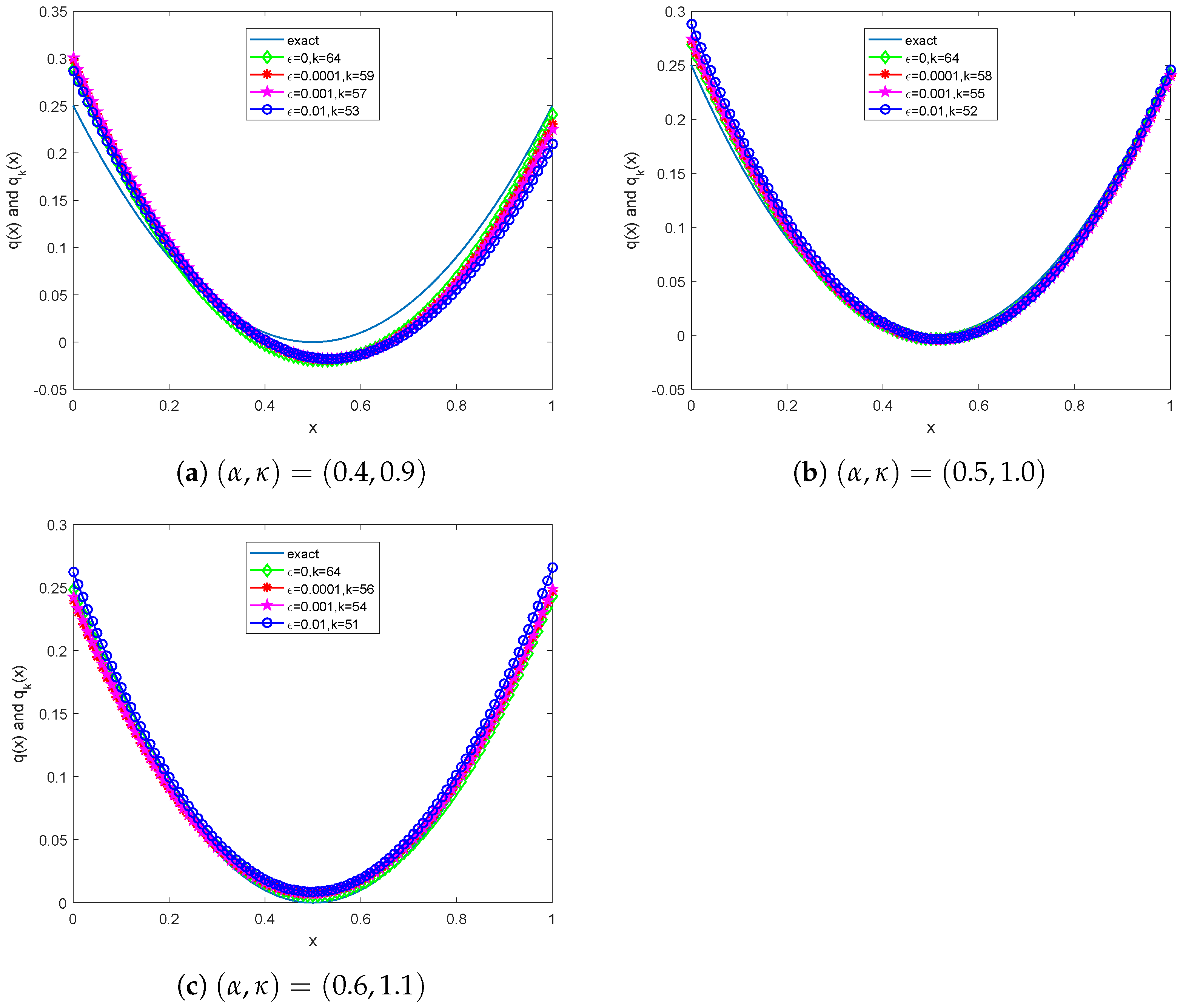
5. Numerical Experiments

In this section, we give three numerical examples to illustrate the effectiveness of the numerical inversion algorithm presented in the above section. And, in all the numerical experiments, we always take $\mathit{\mu }\left(t\right)=sin(2\mathit{\pi }t)$ and $T=1$. The spatial and time steps are always taken to be $h=0.01$ and $\mathit{\tau }=0.01$ when the finite difference method is used to solve the direct problem. The regularization parameters are taken to be

$${\mathit{\mu }}_k=\frac{1}{1+exp\left({\mathit{\beta }}_0\left(k-k_0\right)\right)}\mathrm{and}{\mathit{\lambda }}_k=\frac{1}{1+exp\left({\mathit{\beta }}_1\left(k-k_1\right)\right)},$$

where k is the iteration step, $k_i$ and ${\mathit{\beta }}_i>0(i=0,1)$ are the adjust parameters, and they are taken to be ${\mathit{\beta }}_0=0.45$, ${\mathit{\beta }}_1=0.6$, $k_0=4$, and $k_1=3$. Moreover, random noise is added to the exact data in the following way:

$$d^{\mathit{\delta }}=d+\mathit{ϵ}d\left(2rand\left(size\left(d\right)\right)-1\right).$$

(54)

In the iteration process, the well-known discrepancy principle is adopted to cease the iterations, that is, the iteration will stop at the kth step and k satisfies the inequality

$$E_k\le \mathit{\eta }\mathit{\delta }<E_{k-1},$$

(55)

where $\mathit{\eta }>1$ is a constant and can be taken heuristically to be 1.01. If the noise level is 0, then we take $k=64$ for all the examples. To show the accuracy of the numerical solutions, we compute the approximate errors defined by

$$r{e}_k=\frac{{∥q_k\left(x\right)-q\left(x\right)∥}_{L^2(0,1)}}{{\parallel q\left(x\right)\parallel }_{L^2(0,1)}}+\frac{{∥b^k-b∥}_2}{{\parallel b\parallel }_2},$$

(56)

where $q_k\left(x\right)$ and $b_k$ are the regularization solutions of $q\left(x\right)$ and b in the inverse problem, respectively.

Example 1. 

Suppose $q\left(x\right)=C$, where C is a positive constant. In this example, we take ${\Phi }^J=\left\{1\right\}$, $\mathit{\omega }\left(x\right)=1$, and initial guesses $b_0=(0.01,0.01)$ and $q_0=0$ for the numerical simulations. The inverse results for the various noise levels are shown in

Table 1. The inverse results of Example 1 for various noise levels.

$\mathit{ϵ}$	$(\mathit{q},\mathit{\alpha },\mathit{\kappa })$
	(1.0, 0.4, 0.9)	(2.0, 0.5, 1.0)	(2.5, 0.6, 1.1)
0	(1.0000, 0.4000, 0.9000)	(2.0000, 0.5000, 1.0000)	(2.5000, 0.6000, 1.1000)
0.0001	(0.9999, 0.4001, 0.8999)	(2.0000, 0.5000, 0.9999)	(2.5001, 0.6000, 1.0999)
0.001	(0.9993, 0.4001, 0.8991)	(1.9996, 0.5002, 0.9991)	(2.4998, 0.6002, 1.0993)
0.01	(0.9913, 0.4017, 0.8895)	(1.9959, 0.5019, 0.9898)	(2.4975, 0.6019, 1.0906)

and

Table 2. Relative errors $r{e}_k$ and stopping steps k with different noise levels in Example 1.

${\mathit{re}}_{\mathit{k}}\left(\mathit{k}\right)$
$(\mathit{q},\mathit{\alpha },\mathit{\kappa })$	$\mathit{ϵ}$
	0	0.0001	0.001	0.01
(1.0, 0.4, 0.9)	$2.0295\times {10}^{-12}$ (64)	$1.6549\times {10}^{-4}$ (30)	$1.6633\times {10}^{-3}$ (29)	$1.9495\times {10}^{-2}$ (27)
(2.0, 0.5, 1.0)	$4.3885\times {10}^{-13}$ (64)	$9.67791\times {10}^{-5}$ (31)	$9.2282\times {10}^{-4}$ (30)	$1.1343\times {10}^{-2}$ (28)
(2.5, 0.6, 1.1)	$9.0585\times {10}^{-14}$ (64)	$6.6295\times {10}^{-5}$ (30)	$6.7036\times {10}^{-4}$ (29)	$8.5622\times {10}^{-3}$ (27)

.

Example 2. 

The exact potential is $q\left(x\right)=\frac{1}{4}-x+x^2$. Here, we take ${\Phi }^J=\{1,x,x^2\}$, $\mathit{\omega }\left(x\right)=\frac{1}{25}{(x-1)}^{2}cos(2\mathit{\pi }(1-x))$, and initial guesses $b_0=(0.01,0.01)$ and $q_0=0$ for the numerical simulations. The inverse results for the various noise levels are shown in

Table 3. The inverse results of Example 2 for various noise levels.

$\mathit{ϵ}$	$(\mathit{q},\mathit{\alpha },\mathit{\kappa })$
	(0.4, 0.9)	(0.5, 1.0)	(0.6, 1.1)
0	(0.3998, 0.9002)	(0.5000, 1.0021)	(0.6000, 1.1012)
0.0001	(0.3998, 0.9021)	(0.5000, 1.0024)	(0.6001, 1.1003)
0.001	(0.3999, 0.9027)	(0.5000, 1.0029)	(0.6000, 1.1009)
0.01	(0.3999, 0.8997)	(0.4999, 1.0055)	(0.5999, 1.1048)

and

Table 4. Relative errors $r{e}_k$ and stopping steps k with different noise levels in Example 2.

${\mathit{re}}_{\mathit{k}}\left(\mathit{k}\right)$
$(\mathit{\alpha },\mathit{\kappa })$	$\mathit{ϵ}$
	0	0.0001	0.001	0.01
(0.4, 0.9)	$1.7017\times {10}^{-1}$ (64)	$2.0599\times {10}^{-1}$ (59)	$2.2145\times {10}^{-1}$ (57)	$2.2885\times {10}^{-1}$ (53)
(0.5, 1.0)	$7.5477\times {10}^{-2}$ (64)	$8.6859\times {10}^{-2}$ (58)	$9.5382\times {10}^{-2}$ (55)	$1.3022\times {10}^{-1}$ (52)
(0.6, 1.1)	$3.6931\times {10}^{-2}$ (64)	$4.8702\times {10}^{-2}$ (56)	$4.7942\times {10}^{-2}$ (54)	$9.8544\times {10}^{-2}$ (51)

and Figure 1.

Example 3. 

The exact potential is $q\left(x\right)=1+cos(2\mathit{\pi }x)$. In this example, we take ${\Phi }^J=\{1,cos(\mathit{\pi }x),cos(2\mathit{\pi }x)\}$, $\mathit{\omega }\left(x\right)=\frac{52}{11}(x-\frac{2}{13})(x-\frac{3}{4})$, and the initial guesses $b_0=(0.01,0.01)$ and $q_0=0$ for the numerical simulations. The inverse results for the various noise levels are shown in

Table 5. The inverse results of Example 3 for various noise levels.

$\mathit{ϵ}$	$(\mathit{q},\mathit{\alpha },\mathit{\kappa })$
	(0.4, 0.9)	(0.5, 1.0)	(0.6, 1.1)
0	(0.3998, 0.9105)	(0.4997, 1.0142)	(0.5996, 1.1156)
0.0001	(0.3999, 0.9106)	(0.4997, 1.0141)	(0.5996, 1.1169)
0.001	(0.3999, 0.9110)	(0.4998, 1.0144)	(0.5997, 1.1171)
0.01	(0.3995, 0.9171)	(0.4998, 1.0185)	(0.5987, 1.1219)

and

Table 6. Relative errors $r{e}_k$ and stopping steps k with different noise levels in Example 3.

${\mathit{re}}_{\mathit{k}}\left(\mathit{k}\right)$
$(\mathit{\alpha },\mathit{\kappa })$	$\mathit{ϵ}$
	0	0.0001	0.001	0.01
(0.4, 0.9)	$6.4558\times {10}^{-2}$ (64)	$6.4581\times {10}^{-2}$ (55)	$6.5082\times {10}^{-2}$ (53)	$7.3998\times {10}^{-2}$ (51)
(0.5, 1.0)	$8.0963\times {10}^{-2}$ (64)	$8.0440\times {10}^{-2}$ (53)	$8.0668\times {10}^{-2}$ (51)	$8.5009\times {10}^{-2}$ (49)
(0.6, 1.1)	$8.3986\times {10}^{-2}$ (64)	$9.1304\times {10}^{-2}$ (51)	$9.1397\times {10}^{-2}$ (50)	$9.7026\times {10}^{-2}$ (47)

and Figure 2.

The numerical results in Examples 1–3 show that the presented inversion method is effective for noise free data, and it can obtain satisfactory approximations of the fractional order, the potential, and the Robin coefficient when the noise level does not exeed $1\%$.

6. Conclusions

In this paper, we simultaneously identified the fractional order, the potential function, and the Robin coefficient in a time-fractional diffusion equation with a symmetric potential from an additional integral condition. And, we established the uniqueness of the considered identification problem by using the asymptotic behavior of the Mittag-Leffler function and the methods of Laplace transforms and analytic continuation. We also proved the existence and uniqueness of the weak solution for the forward problem. Finally, we applied the Levenberg–Marquardt regularization method with regularization parameters selected by a sigmoid-type function to simultaneously recover the fractional order, the potential, and the Robin coefficient. Numerical experiments for three test cases were given to demonstrate the effectiveness of the presented method.

References

1. Sakamoto, K.; Yamamoto, M. Inverse source problem with a final overdetermination for a fractional diffusion equation. Math. Control Relat. Fields 2011, 1, 509–518. [Google Scholar] [CrossRef]
2. Hendy, A.S.; van Bockstal, K. On a reconstruction of a solely time-dependent source in a time-fractional diffusion equation with non-smooth solutions. J. Sci. Comput. 2022, 90, 41. [Google Scholar] [CrossRef]
3. Partohaghighi, M.; Karatas Akgül, E.; Weber, G.W.; Yao, G.; Akgül, A. Recovering source term of the time-fractional diffusion equation. Pramana 2021, 95, 153. [Google Scholar] [CrossRef]
4. Zhang, Z.; Zhou, Z. Recovering the potential term in a fractional diffusion equation. IMA J. Appl. Math. 2017, 82, 579–600. [Google Scholar] [CrossRef]
5. Wang, J.G.; Ran, Y.H.; Yuan, Z.B. Uniqueness and numerical scheme for the Robin coefficient identification of the time-fractional diffusion equation. Comput. Math. Appl. 2018, 75, 4107–4114. [Google Scholar] [CrossRef]
6. Wei, T.; Zhang, Z.Q. Robin coefficient identification for a time-fractional diffusion equation. Inverse Probl. Sci. Eng. 2016, 24, 647–666. [Google Scholar] [CrossRef]
7. Wei, T.; Liao, K. Identifying a time-dependent zeroth-order coefficient in a time-fractional diffusion-wave equation by using the measured data at a boundary point. Appl. Anal. 2022, 101, 6522–6547. [Google Scholar] [CrossRef]
8. Wei, T.; Yan, X.B. Uniqueness for identifying a space-dependent zeroth-order coefficient in a time-fractional diffusion-wave equation from a single boundary point measurement. Appl. Math. Lett. 2021, 112, 106814. [Google Scholar] [CrossRef]
9. Wei, T.; Luo, Y. A generalized quasi-boundary value method for recovering a source in a fractional diffusion-wave equation. Inverse Probl. 2022, 38, 045001. [Google Scholar] [CrossRef]
10. Sun, L.; Yan, X.; Liao, K. Simultaneous inversion of a fractional order and a space source term in an anomalous diffusion model. J. Inverse III-Posed Probl. 2022, 30, 791–805. [Google Scholar] [CrossRef]
11. Ruan, Z.; Zhang, W.; Wang, Z. Simultaneous inversion of the fractional order and the space-dependent source term for the time-fractional diffusion equation. Appl. Math. Comput. 2018, 328, 365–379. [Google Scholar] [CrossRef]
12. Ruan, Z.; Zhang, S. Simultaneous inversion of time-dependent source term and fractional order for a time-fractional diffusion equation. J. Comput. Appl. Math. 2020, 368, 112566. [Google Scholar] [CrossRef]
13. Jing, X.; Peng, J. Simultaneous uniqueness for an inverse problem in a time-fractional diffusion equation. Appl. Math. Lett. 2020, 109, 106558. [Google Scholar] [CrossRef]
14. Sun, L.L.; Li, Y.S.; Zhang, Y. Simultaneous inversion of the potential term and the fractional orders in a multi-term time-fractional diffusion equation. Inverse Probl. 2021, 37, 055007. [Google Scholar] [CrossRef]
15. Sun, L.; Wei, T. Identification of the zeroth-order coefficient in a time fractional diffusion equation. Appl. Numer. Math. 2017, 111, 160–180. [Google Scholar] [CrossRef]
16. Sun, L.; Zhang, Y.; Wei, T. Recovering the time-dependent potential function in a multiterm time-fractional diffusion equation. Appl. Numer. Math. 2019, 135, 228–245. [Google Scholar] [CrossRef]
17. Jiang, S.Z.; Wu, Y.J. Recovering a time-dependent potential function in a multi-term time fractional diffusion equation by using a nonlinear condition. J. Inverse III-Posed Probl. 2021, 29, 233–248. [Google Scholar] [CrossRef]
18. Jin, B.; Zhou, Z. Recovering the potential and order in one-dimensional time-fractional diffusion with unknown initial condition and source. Inverse Probl. 2021, 37, 105009. [Google Scholar] [CrossRef]
19. Yan, X.; Wei, T. Identifying a fractional order and a time-dependent coefficient in a time-fractional diffusion wave equation. J. Comput. Appl. Math. 2023, 424, 114995. [Google Scholar] [CrossRef]
20. Yan, X.; Zhang, Z.; Wei, T. Simultaneous inversion of a time-dependent potential coefficient and a time source term in a time fractional diffusion-wave equation. Chaos Solitons Fractals 2022, 157, 111901. [Google Scholar] [CrossRef]
21. Wei, T.; Zhang, Y.; Gao, D. Identification of the zeroth-order coefficient and fractional order in a time-fractional reaction-diffusion-wave equation. Math. Methods Appl. Sci. 2023, 46, 142–166. [Google Scholar] [CrossRef]
22. Bogachev, V.I.; Ruas, M.A.S. Measure Theory; Springer: Berlin/Heidelberg, Germany, 2007. [Google Scholar]
23. Freiling, G.; Yurko, V.A. Inverse Sturm-Liouville Problems and Their Applications; NOVA Science Publishers: New York, NY, USA, 2001. [Google Scholar]
24. Sakamoto, K.; Yamamoto, M. Initial value/boundary value problems for fractional diffusion-wave equations and applications to some inverse problems. J. Math. Anal. Appl. 2011, 382, 426–447. [Google Scholar] [CrossRef]
25. Jin, B. Fractional Differential Equations: An Approach Via Fractional Derivatives; Springer: Berlin/Heidelberg, Germany, 2022. [Google Scholar]
26. Kilbas, A.; Srivastava, H.; Trujillo, J. Theory and Applications of Fractional Differential Equations; Elsevier: Amsterdam, The Netherlands, 2006. [Google Scholar]
Figure 1. Numerical inversions of the potential for various noise levels in Example 2.
Fractalfract 07 00778 g001
Figure 2. Numerical inversions of the potential for various noise levels in Example 3.
Fractalfract 07 00778 g002