A Spectral Collocation Method for Solving the Non-Linear Distributed-Order Fractional Bagley–Torvik Differential Equation

Abstract

One of the issues in numerical solution analysis is the non-linear distributed-order fractional Bagley–Torvik differential equation (DO-FBTE) with boundary and initial conditions. We solve the problem by proposing a numerical solution based on the shifted Legendre Gauss–Lobatto (SL-GL) collocation technique. The solution of the DO-FBTE is approximated by a truncated series of shifted Legendre polynomials, and the SL-GL collocation points are employed as interpolation nodes. At the SL-GL quadrature points, the residuals are computed. The DO-FBTE is transformed into a system of algebraic equations that can be solved using any conventional method. A set of numerical examples is used to verify the proposed scheme’s accuracy and compare it to existing findings.

1. Introduction

Fractional calculus (FC), which has disparate applications in engineering and physics, has captivated researchers over the last three decades. FC is utilized in various applications, including chemical physics, image processing [1], dynamical system control theory, electrical networks, optics, signal processing, probability, and statistics [2]. Linear and non-linear fractional integro-differential equations have extensive engineering and natural sciences applications. Various numerical approaches have been developed to find approximate solutions for spatial–temporal, biological, epidemic, boundary value, and physical modeling problems where analytical solutions are not available.

The distributed-order fractional Bagley–Torvik differential equation is a specific mathematical model used to describe complex dynamic systems with distributed-order fractional derivatives. This equation has applications in various fields, including physics, engineering, and economics. The equation itself can be quite complex, and its solutions can have a wide range of implications depending on the specific parameters and initial conditions.

Predicting precisely what society will derive from the solutions of this equation is challenging, as it depends on the context and how the equation is applied. Society can benefit from research related to distributed-order fractional Bagley–Torvik differential equations through improved understanding, better control of complex systems, innovative engineering solutions, enhanced economic modeling, and advancements in various fields. However, the specific applications and benefits will depend on the context and the problem being addressed.

This study introduces a shifted Legendre–Gauss collocation (SLC-G-C) method for solving the non-linear DO-FBTE, which is defined as follows:

$${\delta }_1\left(\varrho \right)D^2\mathcal{X}\left(\varrho \right)+{\delta }_2\left(\varrho \right)D_{\varrho }^{W_1\left({\alpha }_1\right)}\mathcal{X}\left(\varrho \right)+{\delta }_3\left(\varrho \right)D\mathcal{X}\left(\varrho \right)=\eta (\varrho ,\mathcal{X}\left(\varrho \right)),$$

(1)

with initial-value condition,

$${\mathcal{X}}^{\left(i\right)}\left(0\right)=d_i,i=0,1,$$

(2)

and boundary-value,

$$\mathcal{X}\left(0\right)=d_1,\mathcal{X}\left(1\right)=d_2,0<{\alpha }_1<2.$$

(3)

The fractional Bagley–Torvik equation (FBTE) was created using FC concepts, as mentioned in the references [3,4], whereas Mohammadi and Mohyud-Din [5] used operational matrix methods for solving the FBTE. Deshi and Gudodagi [6] adopted the Haar wavelet, while in [7,8] the authors utilized an implicit hybrid and Galerkin method to solve the FBTE. The FBTE has received a great deal of analytical and numerical attention [9,10].

Bagley and Torvik [11] have investigated the movement of a submerged plate that has been bound in a Newtonian fluid and a gas in a fluid, respectively, and established one of the earliest problems of this sort. The frequency-dependent damping materials have been effectively modeled using fractional-order (order 1/2 or 3/2) derivatives. The BTE has been solved by several authors, both numerically and analytically. Morgado et al. [12] used a finite difference for solving distributed-order diffusion equations, while Aminikhah et al. [13] utilized Grunwald–Letnikov and the transform technique for solving distributed-order fractional Bagley–Torvik equations. The author in [14] used Legendre wavelets for solving distributed-order fractional differential equations (DO-FDEs). Jibenja et al. [15] utilized Taylor polynomials and hybrid block-pulse functions to solve DO-FDEs. Maleknejad et al. [16] used the Muntz–Legendre wavelet approach and the Riemann–Liouville fractional integral for solving linear and non-linear DO-FDEs, while Pourbabaee and Saadatmandi [17] used Chebyshev polynomials and the collocation method to solve DO-FDEs. In [18], the author utilized an operational technique and Chebyshev wavelets for solving DO-FDEs. To the best of our knowledge, no published paper constructs the numerical scheme for the distributed-order non-linear fractional Bagley–Torvik equation with non-smooth initial and boundary conditions. This gap in current research is the motivation for our present work.

Spectral methods [19,20,21] have been widely used in various fields for forty years. Firstly, Fourier-expanded spectral techniques have been used in a few contexts, like periodic boundary conditions and simple geometric areas. They have recently made theoretical progress and have provided effective solutions to many different issues. Spectral approaches outperform other numerical techniques in terms of thoroughness and exponential averages of convergence. The essential step in all spectral approaches is to express the solution as a finite series of distinct functions. There are many different kinds of spectral approaches, such as collocation [22], tau [23], Galerkin [24], and Petrov–Galerkin [25]. After that, the coefficients will be selected to reduce the absolute error. During this time, the numerical solution to the spectral collocation approach will be developed to almost satisfy IDEs. However, at the selected locations, the residuals can be allowed to be zero. The collocation technique has been employed successfully in a wide range of scientific and engineering sectors because of its obvious benefits. Because their global nature fits well with the non-local definition of fractional operators, spectral collocation methods offer intriguing possibilities for solving fractional differential equations.

Although the method has disadvantages, such as the fact that it cannot represent physical processes in spectral space and is hard to parallelize on distributed memory computers, it has a high level of accuracy, speed of convergence, and simplicity in solving differential equations. Spectral methods have been applied for solving many types of differential equations; see [26]. On the other hand, spectral methods have been applied to different types of fractional differential equations. The spectral collocation method [27], as the best spectral method in terms of accuracy, has been applied recently for solving different types of fractional partial differential equations and fractional integro-differential equations [28].

The objective of this study is to devise a methodology for resolving non-linear DO-FBTEs considering initial and boundary conditions through the utilization of the Caputo fractional derivative. Firstly, our focus lies in addressing non-linear DO-FBTEs by employing a numerical technique founded on the SL-GL collocation method. Secondly, we employ shifted fractional Legendre–Gauss collocation points as interpolation nodes, expressing the approximate solution as a truncated series of shifted Legendre polynomials (SLPs). The non-linear DO-FBTE residuals are subsequently estimated at the shifted fractional Legendre–Gauss quadrature points. Ultimately, the equation is transformed into an algebraic equation system that is resolved.

The paper is structured as follows: Section 2 presents the preliminaries of the SLPs. Section 3 solves the non-linear DO-FBTE with boundary-value and initial-value problems, while Section 5 presents numerical simulations to demonstrate the effectiveness and precision of the method. Section 6 introduces some observations and conclusions.

2. Mathematical Preliminaries

The LPs ${\mathcal{L}}_{\mathcal{\ell }}\left(\varrho \right),$$\mathsf{\ell }=0,1\dots ,$ were generated using the Rodrigues formula [29]:

$$\begin{array}{cc}\hfill {\mathcal{L}}_{\mathcal{\ell }}\left(\varrho \right)& =\frac{{(-1)}^{\mathcal{\ell }}}{2^{\mathcal{\ell }}\mathcal{\ell }!}{D}^{\mathcal{\ell }}\left({(1-{\varrho }^2)}^{\mathcal{\ell }}\right).\hfill \end{array}$$

(4)

Furthermore, ${\mathcal{L}}_{\mathcal{\ell }}\left(\varrho \right)$ coincides with a polynomial of degree ℓ, resulting in the pth derivative of ${\mathcal{L}}_{\mathcal{\ell }}\left(\varrho \right)$ as:

$$\begin{array}{c}\hfill {\mathcal{L}}_{\mathcal{\ell }}^{\left(p\right)}\left(\varrho \right)=\sum _{\kappa =0(\mathcal{\ell }+\kappa =even)}^{\mathcal{\ell }-p}{C}_p(\mathcal{\ell },\kappa ){\mathcal{L}}_{\kappa }\left(\varrho \right),\end{array}$$

(5)

where

$$C_p(\mathcal{\ell },\kappa )=\frac{2^{p-1}(2\kappa +1)\Gamma \left(\frac{p+\mathcal{\ell }-\kappa }{2}\right)\Gamma \left(\frac{p+\mathcal{\ell }+\kappa +1}{2}\right)}{\Gamma \left(p\right)\Gamma \left(\frac{2-p+\mathcal{\ell }-\kappa }{2}\right)\Gamma \left(\frac{3-p+\mathcal{\ell }+\kappa }{2}\right)}.$$

We obtain orthogonality by following the procedures below:

$${({\mathcal{L}}_{\mathcal{\ell }}\left(\varrho \right),{\mathcal{L}}_l\left(\varrho \right))}_{\chi }=\underset{-1}{\overset{1}{\int }}{\mathcal{L}}_{\mathcal{\ell }}\left(\varrho \right){\mathcal{L}}_l\left(\varrho \right)\chi \left(\varrho \right)=h_{\mathcal{\ell }}{\delta }_{l\mathcal{\ell }},$$

(6)

whereas $\chi \left(\varrho \right)=1$, $h_{\mathcal{\ell }}=\frac{2}{2\mathcal{\ell }+1}.$ To efficiently assess the integrals indicated above, the L-GL quadrature was employed. For every $\Lambda \in S_{2{\nu }_1-1}$$[-1,1]$, we can write:

$$\begin{array}{c}\hfill \underset{-1}{\overset{1}{\int }}\mathcal{X}\left(\varrho \right)d\varrho =\sum _{\mathcal{\ell }=0}^{{\nu }_1}{\varpi }_{{\nu }_1,j}\mathcal{X}\left({\varrho }_{{\nu }_1,\mathcal{\ell }}\right).\end{array}$$

(7)

Take the discrete inner product as an example:

$${(\mathcal{X},\mathcal{X})}_w=\sum _{\mathcal{\ell }=0}^{{\nu }_1}\mathcal{X}\left({\varrho }_{{\nu }_1,\mathcal{\ell }}\right)\mathcal{X}\left({\varrho }_{{\nu }_1,\mathcal{\ell }}\right){\varpi }_{N,j}.$$

(8)

For the L-GL, we find that [30] ${\varrho }_{{\nu }_1,0}=-1$, ${\varrho }_{{\nu }_1,{\nu }_1}=1$, ${\varrho }_{{\nu }_1,\mathcal{\ell }}$$(\mathcal{\ell }=1,\dots ,{\nu }_1-1)$ are the zeros of ${\left(l_{{\nu }_1}\left(\varrho \right)\right)}^{{}^{\prime }}$, and ${\varpi }_{{\nu }_1,\mathcal{\ell }}=\frac{2}{{\nu }_1({\nu }_1+1){\left({\mathcal{L}}_{{\nu }_1}\left({\varrho }_{{\nu }_1,\mathcal{\ell }}\right)\right)}^2},$ where ${\varpi }_{{\nu }_1,\mathcal{\ell }}$ ($0\le \mathcal{\ell }\le {\nu }_1$) and ${\varrho }_{{\nu }_1,\mathcal{\ell }}$ ($0\le \mathcal{\ell }\le {\nu }_1$) are utilized as the Christoffel numbers and the nodes within $[-1,1]$, respectively. To apply these polynomials in the interval $z\in (0,L)$, we determine a shifted Legendre polynomial (SLPs) by utilizing $\varrho ={\displaystyle \frac{2\varrho }{L}}-1$. If we denote by ${\mathcal{L}}_{L,\kappa }\left(\varrho \right)$ the SLPs ${\mathcal{L}}_{\kappa }\left({\displaystyle \frac{2\varrho }{L}}-1\right)$, then ${\mathcal{L}}_{L,\kappa }\left(\varrho \right)$ can be obtained as [29]:

$$(\kappa +1){\mathcal{L}}_{L,\kappa +1}\left(\varrho \right)=(2\kappa +1)(\frac{2\varrho }{L}-1){\mathcal{L}}_{L,\kappa }\left(\varrho \right)-\kappa {\mathcal{L}}_{L,\kappa -1}\left(\varrho \right),\kappa =1,2,\dots .$$

(9)

The SLPs of degree $\kappa$ in analytic form ${\mathcal{L}}_{L,\kappa }\left(\varrho \right)$ are as follows:

$${\mathcal{L}}_{L,\kappa }\left(\varrho \right)=\sum _{\mathcal{\ell }=0}^{\kappa }{(-1)}^{\kappa +\mathcal{\ell }}\frac{(\kappa +\mathcal{\ell })!}{(\kappa -\mathcal{\ell })!{(\mathcal{\ell }!)}^2{\mathcal{L}}^{\mathcal{\ell }}}{\varrho }^{\mathcal{\ell }}.$$

(10)

The orthogonality condition is expressed as:

$${\int }_0^l{\mathcal{L}}_{L,\mathcal{\ell }}\left(\varrho \right){\mathcal{L}}_{L,\mathcal{\ell }}\left(\varrho \right)w_L\left(\varrho \right)d\varrho ={\hslash }_{\mathcal{\ell }}{\delta }_{\mathcal{\ell }\mathcal{\ell }},$$

(11)

where $w_L\left(\varrho \right)=1\mathrm{and}{\hslash }_{\mathcal{\ell }}={\displaystyle \frac{L}{2\mathcal{\ell }+1}}.$ A square integrable function $\mathcal{X}\left(\varrho \right)$ in the interval $(0,l)$ can be written in terms of SLPs as:

$$\mathcal{X}\left(\varrho \right)=\sum _{\mathcal{\ell }=0}^{\infty }{e}_{\mathcal{\ell }}{\mathcal{L}}_{L,\mathcal{\ell }}\left(\varrho \right),$$

(12)

where the coefficients $e_{\mathcal{\ell }}$ are:

$$e_{\mathcal{\ell }}={\displaystyle \frac{1}{{\hslash }_{\mathcal{\ell }}}}{\int }_0^l\mathcal{X}\left(\varrho \right){\mathcal{L}}_{L,\mathcal{\ell }}\left(t\right)w_L\left(\varrho \right)d\varrho ,\mathcal{\ell }=0,1,2,\dots .$$

(13)

In real-world applications, the first $({\nu }_1+1)$ terms of the SLPs are utilized. As a consequence, $\mathcal{X}\left(\varrho \right)$ looks like this:

$${\mathcal{X}}_{{\nu }_1}\left(\varrho \right)\simeq \sum _{\mathcal{\ell }=0}^{{\nu }_1}{e}_{\mathcal{\ell }}{\mathcal{L}}_{L,\mathcal{\ell }}\left(\varrho \right).$$

(14)

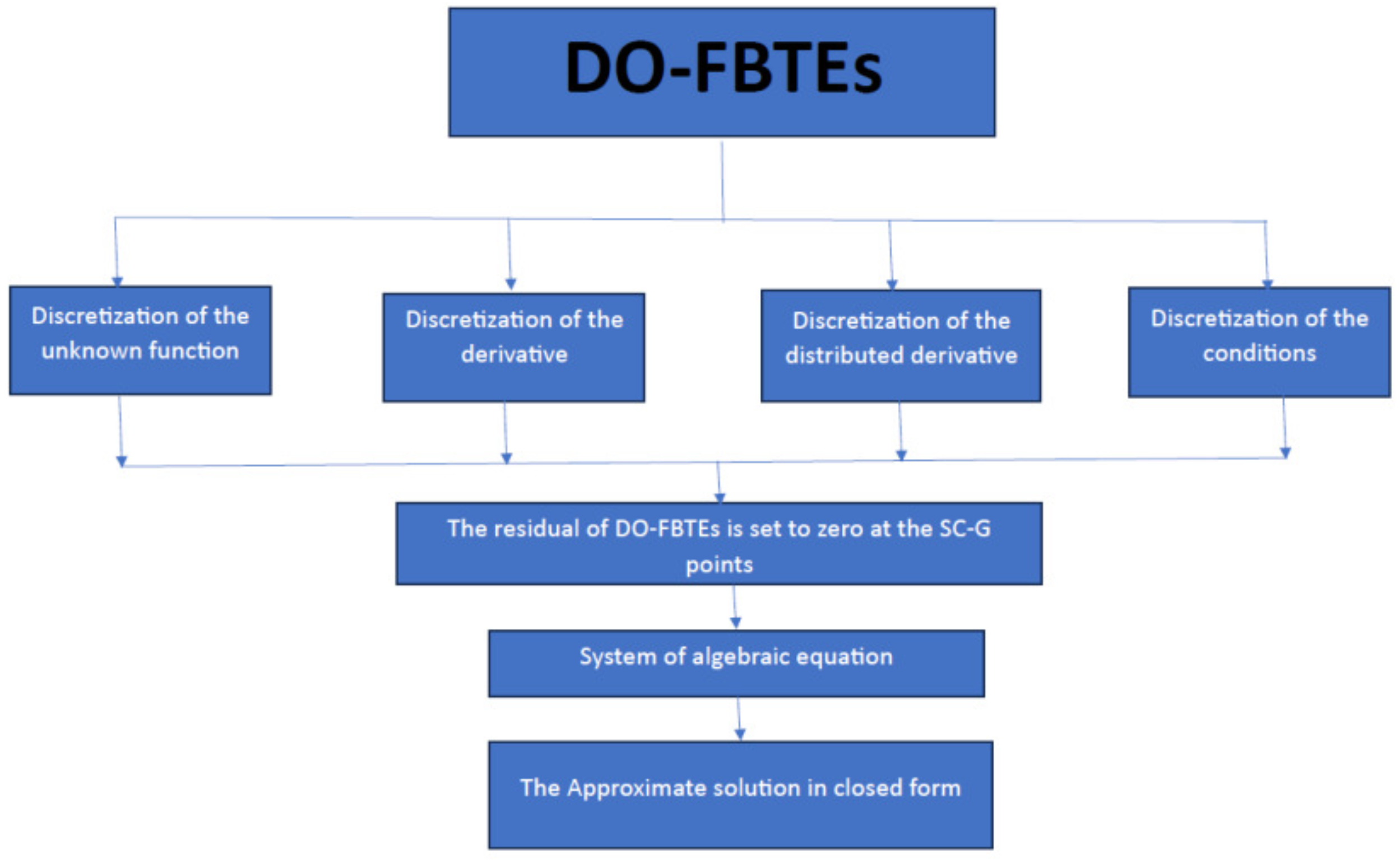
3. Spectral Collocation Approach to Solve the Non-Linear DO-FBTEs

3.1. The Initial-Value Problem

We propose the following numerical method for solving non-linear DO-FBTEs with initial conditions:

$${\delta }_1\left(\varrho \right)D^2\mathcal{X}\left(\varrho \right)+{\delta }_2\left(\varrho \right)D_{\varrho }^{W_1\left({\alpha }_1\right)}\mathcal{X}\left(\varrho \right)+{\delta }_3\left(\varrho \right)D\mathcal{X}\left(\varrho \right)=\eta (\varrho ,\mathcal{X}\left(\varrho \right)),$$

(15)

$${\mathcal{X}}^{\left(i\right)}\left(0\right)=d_i,i=0,1,0<{\alpha }_1<2,$$

(16)

where

$$D_{\varrho }^{W_1\left({\alpha }_1\right)}\mathcal{X}\left(\varrho \right)={\int }_0^1{W}_1\left({\alpha }_1\right)D^{{\alpha }_1}\mathcal{X}\left(\varrho \right)d{\alpha }_1,$$

(17)

$\mathcal{X}\left(\varrho \right)$ is an unknown function. The functions ${\sigma }_1\left(\varrho \right)$, ${\delta }_1\left(\varrho \right)$, ${\delta }_2\left(\varrho \right)$, ${\delta }_3\left(\varrho \right)$ are well-known, and $D^{{\alpha }_1}\mathcal{X}\left(\varrho \right)$ is the Caputo fractional derivative of order ${\alpha }_1$.

Definition 1.

The Caputo derivative [31] of order ${\alpha }_1$ is defined as follows:

$$\begin{array}{c}\hfill D^{{\alpha }_1}\mathcal{X}\left(\varrho \right)=\frac{1}{\Gamma (\gamma -{\alpha }_1)}{\int }_0^{\varrho }{(\varrho -\epsilon )}^{\gamma -{\alpha }_1-1}{\mathcal{X}}^{\left(\gamma \right)}\left(\epsilon \right)d\epsilon ,\gamma -1<{\alpha }_1\le \gamma ,\varrho >0,\end{array}$$

(18)

where γ is the ceiling function of ${\alpha }_1$.

If ${\mathcal{X}}_{Approx}\left(\varrho \right)$ is defined as an approximation of (15):

$${\mathcal{X}}_{Approx}\left(\varrho \right)=\sum _{\mathcal{\ell }=0}^{{\nu }_1}{a}_{\mathcal{\ell }}{\mathcal{L}}_{L,\mathcal{\ell }}\left(\varrho \right),$$

(19)

then the derivative $D^{{\alpha }_1}$ of ${\mathcal{X}}_{Approx}\left(\varrho \right)$ is:

$$\begin{array}{c}\hfill D^{{\alpha }_1}{\mathcal{X}}_{Approx}\left(\varrho \right)=\sum _{\mathcal{\ell }=0}^{{\nu }_1}{a}_{\mathcal{\ell }}{D}^{{\alpha }_1}\left({\mathcal{L}}_{L,\mathcal{\ell }}\left(\varrho \right)\right).\end{array}$$

(20)

By utilizing the Caputo derivative of ${\alpha }_1$ given in Definition 18, we have:

$$\begin{array}{cc}\hfill D^{{\alpha }_1}{\varrho }^{\mathcal{\ell }}=& \frac{1}{\Gamma (1-{\alpha }_1)}\underset{0}{\overset{\varrho }{\int }}\frac{{\vartheta }^{(\mathcal{\ell })}}{{(\varrho -\vartheta )}^{{\alpha }_1}}d\vartheta \hfill \\ \hfill =& \frac{{\varrho }^{\mathcal{\ell }-{\alpha }_1}\Gamma (1+\mathcal{\ell })}{\Gamma (1+\mathcal{\ell }-{\alpha }_1)}.\hfill \end{array}$$

(21)

As a result, it follows that:

$$\begin{array}{cc}\hfill D^{{\alpha }_1}{\mathcal{L}}_{L,\mathcal{\ell }}\left(\varrho \right)& =\sum _{\mathcal{\ell }=0}^{{\nu }_1}{(-1)}^{\mathcal{\ell }-{\nu }_1}\frac{({\nu }_1+\mathcal{\ell }-1)!2^{2\mathcal{\ell }}}{({\nu }_1-\mathcal{\ell })!(2\mathcal{\ell })!L^{\mathcal{\ell }}}{D}^{{\alpha }_1}{\varrho }^{\mathcal{\ell }}\hfill \\ \hfill & =\sum _{\mathcal{\ell }=0}^{{\nu }_1}{(-1)}^{\mathcal{\ell }-{\nu }_1}\frac{\mathcal{\ell }!({\nu }_1+\mathcal{\ell }-1)!2^{2\mathcal{\ell }}}{({\nu }_1-\mathcal{\ell })!(2\mathcal{\ell })!L^{\mathcal{\ell }}(\mathcal{\ell }-{\alpha }_1)!}{\varrho }^{\mathcal{\ell }-{\alpha }_1}.\hfill \end{array}$$

(22)

As a result, we have the following:

$$\begin{array}{c}\hfill D^{{\alpha }_1}{\mathcal{X}}_{Approx}\left(\varrho \right)=\sum _{\mathcal{\ell }=0}^{{\nu }_1}{a}_{\mathcal{\ell }}{D}^{{\alpha }_1}\left({\mathcal{L}}_{L,\mathcal{\ell }}\left(\varrho \right)\right)=\sum _{\mathcal{\ell }=0}^{{\nu }_1}{a}_{\mathcal{\ell }}{\Delta }_{L,\mathcal{\ell }}\left(\varrho \right).\end{array}$$

(23)

For any positive integer ${\nu }_1$, let $S_{{\nu }_1}(0,L)$ be the set of all polynomials of degree at most ${\nu }_1$. Based on the SL-GL quadrature, it follows for any $\mathcal{X}\in S_{2{\nu }_1-1}(0,L)$ that

$${\int }_0^L\mathcal{X}\left(\varrho \right)d\varrho =\sum _{i=0}^{{\nu }_1}{\varpi }_{L,{\nu }_1,i}\mathcal{X}\left({\varrho }_{L,{\nu }_1,i}\right),$$

(24)

where ${\varrho }_{L,{\nu }_1,i},{\varpi }_{L,{\nu }_1,i}$ are the nodes and Christoffel numbers of SL-GL interpolation on the interval $[0,L]$, respectively. Meanwhile, using the SL-GL quadrature rule, approximate the integral part on the right-hand side of (17),

$$\begin{array}{cc}\hfill {\int }_0^1{W}_1\left({\alpha }_1\right)D_{\varrho }^{{\alpha }_1}\mathcal{X}\left(\varrho \right)d{\alpha }_1=& {\int }_0^1{W}_1\left({\alpha }_1\right)\sum _{\mathcal{\ell }=0}^{{\nu }_1}{a}_{\mathcal{\ell }}{\Delta }_{L,\mathcal{\ell }}\left(\varrho \right)d{\alpha }_1\hfill \\ \hfill =& \sum _{\mathcal{\ell }=0}^{{\nu }_1}{a}_{\mathcal{\ell }}\left({\int }_0^1{W}_1\left({\alpha }_1\right){\Delta }_{L,\mathcal{\ell }}({\alpha }_1,\varrho )d{\alpha }_1\right)\hfill \\ \hfill =& \sum _{\mathcal{\ell }=0}^{{\nu }_1}\sum _{i=0}^{{\nu }_1}{a}_{\mathcal{\ell }}{\varpi }_{{\nu }_1,i}{W}_1\left({{\alpha }_1}_{{\nu }_1,i}\right){\Delta }_{L,\mathcal{\ell }}({{\alpha }_1}_{{\nu }_1,i},\varrho )\hfill \\ \hfill =& \sum _{\mathcal{\ell }=0}^{{\nu }_1}{a}_{\mathcal{\ell }}{\zeta }_{L,\mathcal{\ell }}\left(\varrho \right).\hfill \end{array}$$

(25)

We approximate $D^2\mathcal{X}\left(\varrho \right)$ and $D\mathcal{X}\left(\varrho \right)$ as:

$$D^2\mathcal{X}\left(\varrho \right)=\sum _{\mathcal{\ell }=0}^{{\nu }_1}{a}_{\mathcal{\ell }}{D}^{\left(2\right)}\left({\mathcal{L}}_{L,\mathcal{\ell }}\left(\varrho \right)\right)=\sum _{\mathcal{\ell }=0}^{{\nu }_1}{c}_{\mathcal{\ell }}{\Omega }_{L,\mathcal{\ell }}\left(\varrho \right),$$

(26)

$$D\mathcal{X}\left(\varrho \right)=\sum _{\mathcal{\ell }=0}^{{\nu }_1}{a}_{\mathcal{\ell }}D\left({\mathcal{L}}_{L,\mathcal{\ell }}\left(\varrho \right)\right)=\sum _{\mathcal{\ell }=0}^{{\nu }_1}{c}_{\mathcal{\ell }}{\xi }_{L,\mathcal{\ell }}\left(\varrho \right).$$

(27)

By utilizing Equations (23), (26) and (27), we rewrite Equation (15) as:

$$\begin{array}{c}\hfill {\delta }_1\left(\varrho \right)\sum _{\mathcal{\ell }=0}^{{\nu }_1}{a}_{\mathcal{\ell }}{\zeta }_{L,\mathcal{\ell }}\left(\varrho \right)+{\delta }_2\left(\varrho \right)\sum _{\mathcal{\ell }=0}^{{\nu }_1}{c}_{\mathcal{\ell }}{\Omega }_{L,\mathcal{\ell }}\left(\varrho \right)+{\delta }_3\left(\varrho \right)\sum _{\mathcal{\ell }=0}^{{\nu }_1}{c}_{\mathcal{\ell }}{\xi }_{L,\mathcal{\ell }}\left(\varrho \right)=\eta (\varrho ,\sum _{\mathcal{\ell }=0}^{{\nu }_1}{a}_{\mathcal{\ell }}{\mathcal{L}}_{L,\mathcal{\ell }}\left(\varrho \right)).\end{array}$$

(28)

The residual of Equation (28) is set to zero by using the SL-GL collocation approach at ${\nu }_1-1,$ of the SL-GL points. By employing Equations (19)–(28), then (15) can be written as:

$$\begin{array}{cc}\hfill {\delta }_1\left(\varrho \right)\sum _{\mathcal{\ell }=0}^{{\nu }_1}{a}_{\mathcal{\ell }}{\zeta }_{L,\mathcal{\ell }}\left({\varrho }_{L,{\nu }_1,i}\right)+{\delta }_2\left(\varrho \right)\sum _{\mathcal{\ell }=0}^{{\nu }_1}{c}_{\mathcal{\ell }}{\Omega }_{L,\mathcal{\ell }}\left({\varrho }_{L,{\nu }_1,i}\right)+{\delta }_3\left(\varrho \right)\sum _{\mathcal{\ell }=0}^{{\nu }_1}{c}_{\mathcal{\ell }}{\xi }_{L,\mathcal{\ell }}\left({\varrho }_{L,{\nu }_1,i}\right)& \\ \hfill =\eta ({\varrho }_{L,{\nu }_1,i},\sum _{\mathcal{\ell }=0}^{{\nu }_1}{a}_{\mathcal{\ell }}{\mathcal{L}}_{L,\mathcal{\ell }}\left({\varrho }_{L,{\nu }_1,i}\right)).\end{array}$$

(29)

Rewriting the previous equation yields:

$$\begin{array}{c}\hfill \sum _{\mathcal{\ell }=0}^{{\nu }_1}{a}_{\mathcal{\ell }}\left[{\delta }_1\left(\varrho \right){\zeta }_{L,\mathcal{\ell }}+{\delta }_2\left(\varrho \right){\Omega }_{L,\mathcal{\ell }}+{\delta }_3\left(\varrho \right){\xi }_{L,\mathcal{\ell }}\right]\left({\varrho }_{L,{\nu }_1,i}\right)=\eta ({\varrho }_{L,{\nu }_1,i},\sum _{\mathcal{\ell }=0}^{{\nu }_1}{a}_{\mathcal{\ell }}{\mathcal{L}}_{L,\mathcal{\ell }}\left({\varrho }_{L,{\nu }_1,i}\right)),i=1,\dots ,{\nu }_1.\end{array}$$

(30)

Therefore, we have:

$$\begin{array}{c}\hfill \sum _{\mathcal{\ell }=0}^{{\nu }_1}{a}_{\mathcal{\ell }}{{\rm Y}}_{L,\mathcal{\ell }}\left({\varrho }_{L,{\nu }_1,i}\right)=\eta ({\varrho }_{L,{\nu }_1,i},\sum _{\mathcal{\ell }=0}^{{\nu }_1}{a}_{\mathcal{\ell }}{\mathcal{L}}_{L,\mathcal{\ell }}\left({\varrho }_{L,{\nu }_1,i}\right)),i=1,\dots ,{\nu }_1,\end{array}$$

(31)

where ${{\rm Y}}_{L,\mathcal{\ell }}=\left[{\delta }_1\left(\varrho \right){\zeta }_{L,\mathcal{\ell }}+{\delta }_2\left(\varrho \right){\xi }_{L,\mathcal{\ell }}+{\delta }_3\left(\varrho \right){\Omega }_{L,\mathcal{\ell }}\right]$. Combining Equations (16) and (19), we obtain:

$$\begin{array}{c}\hfill \sum _{\mathcal{\ell }=0}^{{\nu }_1}{a}_{\mathcal{\ell }}{D}^i{\mathcal{L}}_{L,\mathcal{\ell }}\left(0\right)=d_i,i=0,1.\end{array}$$

(32)

In contrast, we can write:

$$\begin{array}{c}\hfill \sum _{\mathcal{\ell }=0}^{{\nu }_1}{a}_{\mathcal{\ell }}{D}^0{\mathcal{L}}_{L,\mathcal{\ell }}\left(0\right)=\sum _{\mathcal{\ell }=0}^{{\nu }_1}{(-1)}^{\mathcal{\ell }}{a}_{\mathcal{\ell }}=d_0,\end{array}$$

(33)

$$\begin{array}{c}\hfill \sum _{\mathcal{\ell }=0}^{{\nu }_1}{a}_{\mathcal{\ell }}D{\mathcal{L}}_{L,\mathcal{\ell }}\left(0\right)=\sum _{\mathcal{\ell }=0}^{{\nu }_1}\frac{{(-1)}^{\mathcal{\ell }-1}\Gamma (\mathcal{\ell }+1)(\mathcal{\ell }+1)}{L(\mathcal{\ell }-1)!\Gamma \left(2\right)}{a}_{\mathcal{\ell }}=d_1.\end{array}$$

(34)

The Equations (31), (33) and (34) represent a system of $({\nu }_1+1)$ algebraic equations in the unknowns $a_{\mathcal{\ell }},i=0,\dots ,{\nu }_1$:

$$\left\{\begin{array}{c}\begin{array}{cc}\hfill & \sum _{\mathcal{\ell }=0}^{{\nu }_1}{(-1)}^{\mathcal{\ell }}{a}_{\mathcal{\ell }}=d_0,\hfill \\ \hfill & \sum _{\mathcal{\ell }=0}^{{\nu }_1}\frac{{(-1)}^{\mathcal{\ell }-1}\Gamma (\mathcal{\ell }+1)(\mathcal{\ell }+1)}{L(\mathcal{\ell }-1)!\Gamma \left(2\right)}{a}_{\mathcal{\ell }}=d_1,\hfill \\ \hfill & \sum _{\mathcal{\ell }=0}^{{\nu }_1}{a}_{\mathcal{\ell }}{{\rm Y}}_{L,\mathcal{\ell }}\left({\varrho }_{L,{\nu }_1,i}\right)=\eta ({\varrho }_{L,{\nu }_1,i},\sum _{\mathcal{\ell }=0}^{{\nu }_1}{a}_{\mathcal{\ell }}{\mathcal{L}}_{L,\mathcal{\ell }}\left({\varrho }_{L,{\nu }_1,i}\right)),i=1,\dots ,{\nu }_1.\hfill \end{array}\hfill \end{array}\right.$$

(35)

Lastly, the system is easily solved. As a result, ${\mathcal{X}}_{Approx}$ can be written in closed form.

3.2. The Boundary-Value Problem

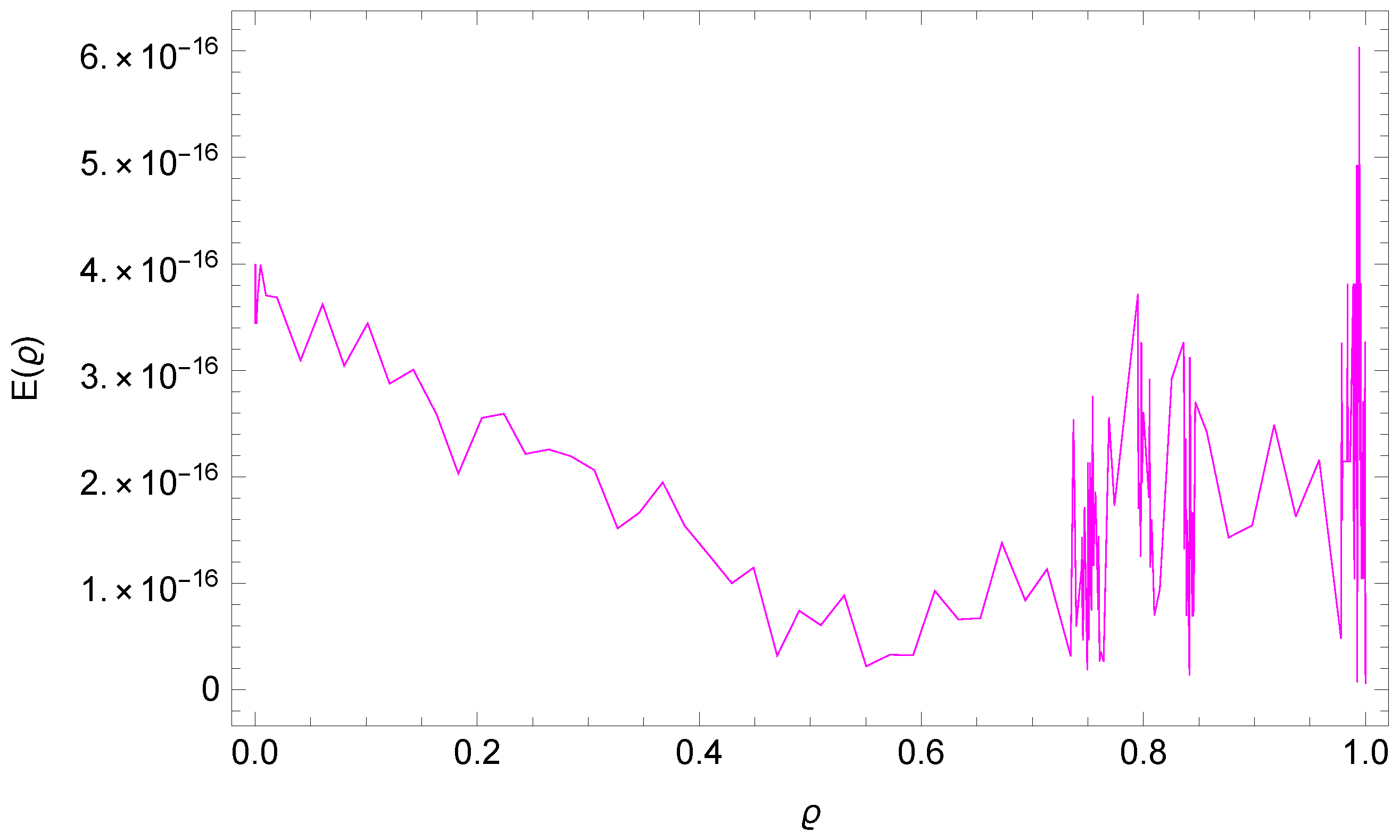
The technique is extended to solve non-linear DO-FBTEs with boundary values:

$${\delta }_1\left(\varrho \right)D^2\mathcal{X}\left(\varrho \right)+{\delta }_2\left(\varrho \right)D\mathcal{X}\left(\varrho \right)+{\delta }_3\left(\varrho \right)D^{{\sigma }_1\left(\varrho \right)}\mathcal{X}\left(\varrho \right)=\Theta (\varrho ,\mathcal{X}\left(\varrho \right)),$$

(36)

subject to,

$$\mathcal{X}\left(0\right)=d_1,\mathcal{X}\left(1\right)=d_2,0<{\alpha }_1<2,$$

(37)

where $\mathcal{X}\left(\varrho \right)$ is unknown, and the functions ${\sigma }_1\left(\varrho \right)$, ${\delta }_1\left(\varrho \right)$, ${\delta }_2\left(\varrho \right)$, and ${\delta }_3\left(\varrho \right)$ are well-known.

We obtain the following results after a procedure similar to the one described in the preceding subsection:

$$\begin{array}{c}\hfill \sum _{\mathcal{\ell }=0}^{{\nu }_1}{a}_{\mathcal{\ell }}{\Psi }_{L,\mathcal{\ell }}\left({\varrho }_{L,{\nu }_1,i}\right)=\Theta ({\varrho }_{L,{\nu }_1,i},\sum _{\mathcal{\ell }=0}^{{\nu }_1}{a}_{\mathcal{\ell }}{\mathcal{L}}_{L,\mathcal{\ell }}\left({\varrho }_{L,{\nu }_1,i}\right)),i=1,\dots ,{\nu }_1,\end{array}$$

(38)

where ${\Psi }_{L,\mathcal{\ell }}=\left[{\delta }_1\left(\varrho \right){\Delta }_{L,\mathcal{\ell }}+{\delta }_2\left(\varrho \right){\xi }_{L,\mathcal{\ell }}+{\delta }_3\left(\varrho \right){\Omega }_{L,\mathcal{\ell }}\right]$. We then combine Equations (37) and (19), and set to zero the residual of (38) at ${\nu }_1+1$ SL-GL points:

$$\left\{\begin{array}{c}\begin{array}{cc}\hfill & \sum _{\mathcal{\ell }=0}^{{\nu }_1}{a}_{\mathcal{\ell }}{\mathcal{L}}_{L,\mathcal{\ell }}\left(0\right)=d_1,\hfill \\ \hfill & \sum _{\mathcal{\ell }=0}^{{\nu }_1}{a}_{\mathcal{\ell }}{\mathcal{L}}_{L,\mathcal{\ell }}\left(1\right)=d_2,\hfill \\ \hfill & \sum _{\mathcal{\ell }=0}^{{\nu }_1}{a}_{\mathcal{\ell }}{\Psi }_{L,\mathcal{\ell }}\left({\varrho }_{L,{\nu }_1,i}\right)=\Theta ({\varrho }_{L,{\nu }_1,i},\sum _{\mathcal{\ell }=0}^{{\nu }_1}{a}_{\mathcal{\ell }}{\mathcal{L}}_{L,\mathcal{\ell }}\left({\varrho }_{L,{\nu }_1,i}\right)),i=1,\dots ,{\nu }_1.\hfill \end{array}\hfill \end{array}\right.$$

(39)

The resulting system of algebraic equations can be easily solved:

$${\mathcal{X}}_{Approx}\left(\varrho \right)=\sum _{\mathcal{\ell }=0}^{{\nu }_1}{a}_{\mathcal{\ell }}{\mathcal{L}}_{L,\mathcal{\ell }}\left(\varrho \right).$$

(40)

Figure 1 shows a flowchart outlining the stages of our methodology.

4. Error Analysis

In this section, we give some useful lemmas that will play a significant role in the convergence analysis later. Let us first introduce some notations that will be used. Let $I:=(-1,1)$ and $L^2\left(I\right)$ be the space of measurable functions whose square is the Lebesgue integrable in I relative to the weight function $\mathcal{X}\left(\varrho \right)$. The inner product and norm are defined by

$${(\mathcal{X},\psi )}_{\mathcal{X}\left(I\right)}={\int }_{-1}^1\mathcal{X}\left(\varrho \right)\psi \left(\varrho \right)\mathcal{X}d\varrho ,{\parallel \mathcal{X}\parallel }_{L_{\mathcal{X}}^2}={(\mathcal{X},\mathcal{X})}_{\mathcal{X}}^{\frac{1}{2}}.$$

(41)

Definition 2.

For a non-negative integer m, define the weighted Hilbert space [30,32,33]

$$H_{\mathcal{X}\left(I\right)}^m=\mathcal{X}:{\partial }_{\varrho }^k\mathcal{X}\in L_{\mathcal{X}\left(I\right)}^2,0\le k\le m,$$

(42)

with the seminorm and the norm as follows:

$${\parallel \mathcal{X}\parallel }_{m,\mathcal{X}\left(I\right)}=\parallel {\partial }_{\varrho }^k{\mathcal{X}\parallel }_{\mathcal{X}\left(I\right)},{\parallel \mathcal{X}\parallel }_{m,\mathcal{X}\left(I\right)}={\left(\sum _{k=0}^m{\left|\mathcal{X}\right|}_{k,\mathcal{X}\left(I\right)}^2\right)}^{\frac{1}{2}},$$

(43)

$${\parallel \mathcal{X}\parallel }_{H_{\mathcal{X}\left(I\right)}^{m,N}}={\left(\sum _{k=min(m,N+1)}^m{\parallel {\partial }_{\varrho }^k\mathcal{X}\parallel }_{L_{\mathcal{X}\left(I\right)}^2}^2\right)}^2.$$

(44)

Lemma 1.

Assume that $\mathcal{X}\in H_{\mathcal{X}}^m$ and denote $I_{{\nu }_1}\mathcal{X}$ its interpolation polynomial associated with the ${\varrho }_{i=0}^{{\nu }_1}$, namely [30]

$$I_{{\nu }_1}\mathcal{X}\left({\varrho }_i\right)=\mathcal{X}\left({\varrho }_i\right).$$

(45)

Then, the following estimates hold:

$$\parallel \mathcal{X}-I_{{\nu }_1}\mathcal{X}\left(\varrho \right)\parallel =C{{\nu }_1}^{\frac{1}{2}-m}{\left|\mathcal{X}\right|}_{H_{\mathcal{X}}^{m,{\nu }_1}}.$$

(46)

Lemma 2.

Assume that $\mathcal{X}\in H_{\varpi }^m\left(I\right)$ and $I_{{\nu }_1}\mathcal{X}$ denote the interpolation of $\mathcal{X}$ based on $({\nu }_1+1)$ degree with the Gauss–Lobatto points corresponding to the weight function $\mathcal{X}\left(\varrho \right)$ (see [30,34])

$$\parallel D^{\left({\alpha }_1\right)}\mathcal{X}-I_{{\nu }_1}{D}^{\left({\alpha }_1\right)}\mathcal{X}{\parallel }_{L_{\mathcal{X}}^2\left(I\right)}\le C{\nu }_1^{-m}{\left|{\mathcal{X}}^{\left({\alpha }_1\right)}\right|}_{H_{\mathcal{X}}^{m,{\nu }_1}\left(I\right)}.$$

(47)

Theorem 1.

Let $\mathcal{X}\left(\varrho \right)$ be the exact solution of the non-linear DO-FBTE (1), which is assumed to be sufficiently smooth. Let the approximate solution $I_{{\nu }_1}\mathcal{X}\left(\varrho \right)$ be obtained by using the proposed method. If $\mathcal{X}\left(\varrho \right)\in H_{{\nu }_1}\left(I\right)$, then for sufficiently large ${\nu }_1$ the following error estimate holds:

$${\parallel e\left(x\right)\parallel }_{L^{\infty }}\le \frac{1}{L}(C{\nu }_1^{\frac{1}{2}-m}|{\mathcal{X}}^{{}^{″}}{|}_{H_{\mathcal{X}}^{m;{\nu }_1}\left(I\right)}+CK{{\nu }_1}^{-m}|{\mathcal{X}}^{\left({\alpha }_1\right)}{|}_{H_{\mathcal{X}}^{m;{\nu }_1}\left(I\right)}+C{{\nu }_1}^{\frac{1}{2}-m}{\left|{\mathcal{X}}^{{}^{\prime }}\right|}_{H_{\mathcal{X}}^{m;{\nu }_1}\left(I\right)}).$$

(48)

Proof. 

We use ${\mathcal{X}}_i\approx \mathcal{X}\left({\varrho }_i\right)$, $0\le i\le {\nu }_1$, and ${\mathcal{X}}_{{\nu }_1}={\displaystyle \sum _{j=0}^{{\nu }_1}}{\mathcal{X}}_j{F}_j\left(\varrho \right)$ ${\mathcal{X}}_{{\nu }_1}^{{\alpha }_1}={\displaystyle \sum _{j=0}^{{\nu }_1}}{\mathcal{X}}_j{F}_j^{{\alpha }_1}\left(\varrho \right),$ where $Fj,j=0,1,2,\dots ,{\nu }_1$ is the Lagrange interpolation basis function. Consider the Equation (1) and ${\alpha }_1\left(\varrho \right)$ is fractional. By using shifted Legendre–Gauss–Lobatto collocation points ${{\varrho }_i}_{i=0}^{{\nu }_1}$, we have

$${\mathcal{X}}^{{}^{″}}\left(\varrho \right)+D_{\varrho }^{W_1\left({\alpha }_1\right)}\mathcal{X}\left(\varrho \right)+{\mathcal{X}}^{{}^{\prime }}\left(\varrho \right)=\eta (\varrho ,\mathcal{X}\left(\varrho \right)),$$

(49)

$${\mathcal{X}}^{{}^{″}}\left(\varrho \right)+{\int }_0^1{W}_1\left({\alpha }_1\right)D^{{\alpha }_1}\mathcal{X}\left(\varrho \right)d{\alpha }_1+{\mathcal{X}}^{{}^{\prime }}\left(\varrho \right)=\eta (\varrho ,\mathcal{X}\left(\varrho \right)),$$

(50)

the numerical scheme can be written,

$$I_{{\nu }_1}{\mathcal{X}}^{{}^{″}}\left(\varrho \right)+I_{{\nu }_1}{D}_{\varrho }^{W_1\left({\alpha }_1\right)}\mathcal{X}\left(\varrho \right)+I_{{\nu }_1}{\mathcal{X}}^{{}^{\prime }}\left(\varrho \right)=\eta (\varrho ,I_{{\nu }_1}\mathcal{X}\left(\varrho \right)).$$

(51)

$$I_{{\nu }_1}{\mathcal{X}}^{{}^{″}}\left(\varrho \right)+{\int }_0^1{W}_1\left({\alpha }_1\right)I_{{\nu }_1}{D}^{{\alpha }_1}\mathcal{X}\left(\varrho \right)d{\alpha }_1+I_{{\nu }_1}{\mathcal{X}}^{{}^{\prime }}\left(\varrho \right)=\eta (\varrho ,I_{{\nu }_1}\mathcal{X}\left(\varrho \right)).$$

(52)

We subtract (52) from (50), and using the Lipschitz condition to obtain the equation,

$${\mathcal{X}}^{{}^{\prime }}\left(\varrho \right)-I_{{\nu }_1}{\mathcal{X}}^{{}^{″}}\left(\varrho \right)+K(D^{{\alpha }_1}\mathcal{X}\left(\varrho \right)-I_{{\nu }_1}{D}^{{\alpha }_1}\mathcal{X}\left(\varrho \right))+{\mathcal{X}}^{{}^{\prime }}\left(\varrho \right)-I_{{\nu }_1}{\mathcal{X}}^{{}^{\prime }}\left(\varrho \right)=L(\mathcal{X}\left(\varrho \right)-I_{{\nu }_1}\mathcal{X}\left(\varrho \right)),$$

(53)

we can write the previous equation as

$$e\left(x\right)=\frac{1}{L}(J_1+K{J}_2+J_3),$$

(54)

where K and L are Lipschitz constants and $J_1={\mathcal{X}}^{{}^{″}}\left(\varrho \right)-I_{{\nu }_1}{\mathcal{X}}^{{}^{″}}\left(\varrho \right),$$J_2={\mathcal{X}}^{\left({\alpha }_1\right)}\left(\varrho \right)-I_{{\nu }_1}{\mathcal{X}}^{\left({\alpha }_1\right)}\left(\varrho \right),$ $J_3={\mathcal{X}}^{{}^{\prime }}\left(\varrho \right)-I_{{\nu }_1}{\mathcal{X}}^{{}^{\prime }}\left(\varrho \right)$.

From Gronwall inequality, we can write

$${\parallel e\left(x\right)\parallel }_{L_{\infty }}=\frac{1}{L}(\parallel J_1{\parallel }_{L_{\infty }}+K\parallel J_2{\parallel }_{L_{\infty }}+\parallel J_3{\parallel }_{L_{\infty }}).$$

(55)

Using the previous lemma, we have

$$\parallel J_1{\parallel }_{L_{\infty }}\le C{{\nu }_1}^{\frac{1}{2}-m}{\left|{\mathcal{X}}^{{}^{\prime \prime }}\right|}_{H_{\mathcal{X}}^{m;{\nu }_1}\left(I\right)},$$

(56)

$$\parallel J_2{\parallel }_{L_{\infty }}\le C{{\nu }_1}^{-m}{\left|{\mathcal{X}}^{\left({\alpha }_1\right)}\right|}_{H_{\varpi }^{m;{\nu }_1}\left(I\right)},$$

(57)

$$\parallel J_3{\parallel }_{L_{\infty }}\le C{{\nu }_1}^{\frac{1}{2}-m}{\left|{\mathcal{X}}^{{}^{\prime }}\right|}_{H_{\mathcal{X}}^{m;{\nu }_1}\left(I\right)}.$$

(58)

Hence, a combination of Equations (56)–(58) leads to the desired conclusion of this theorem. □

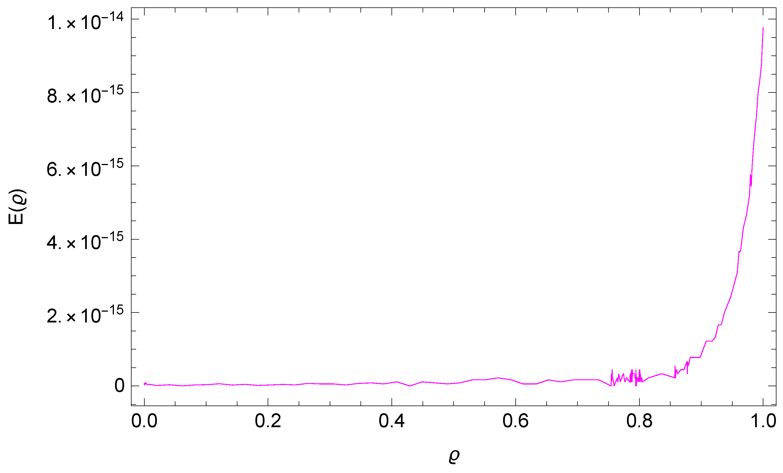
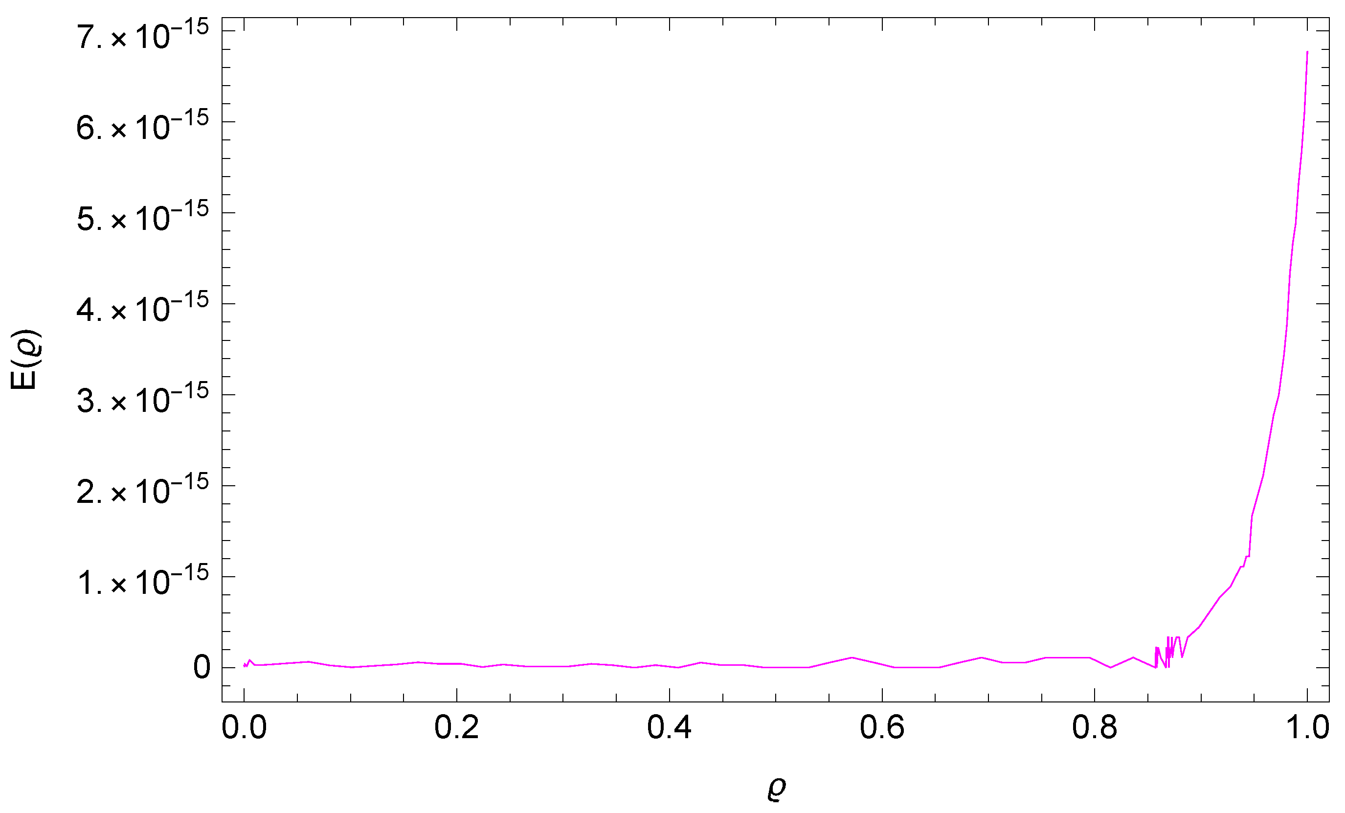
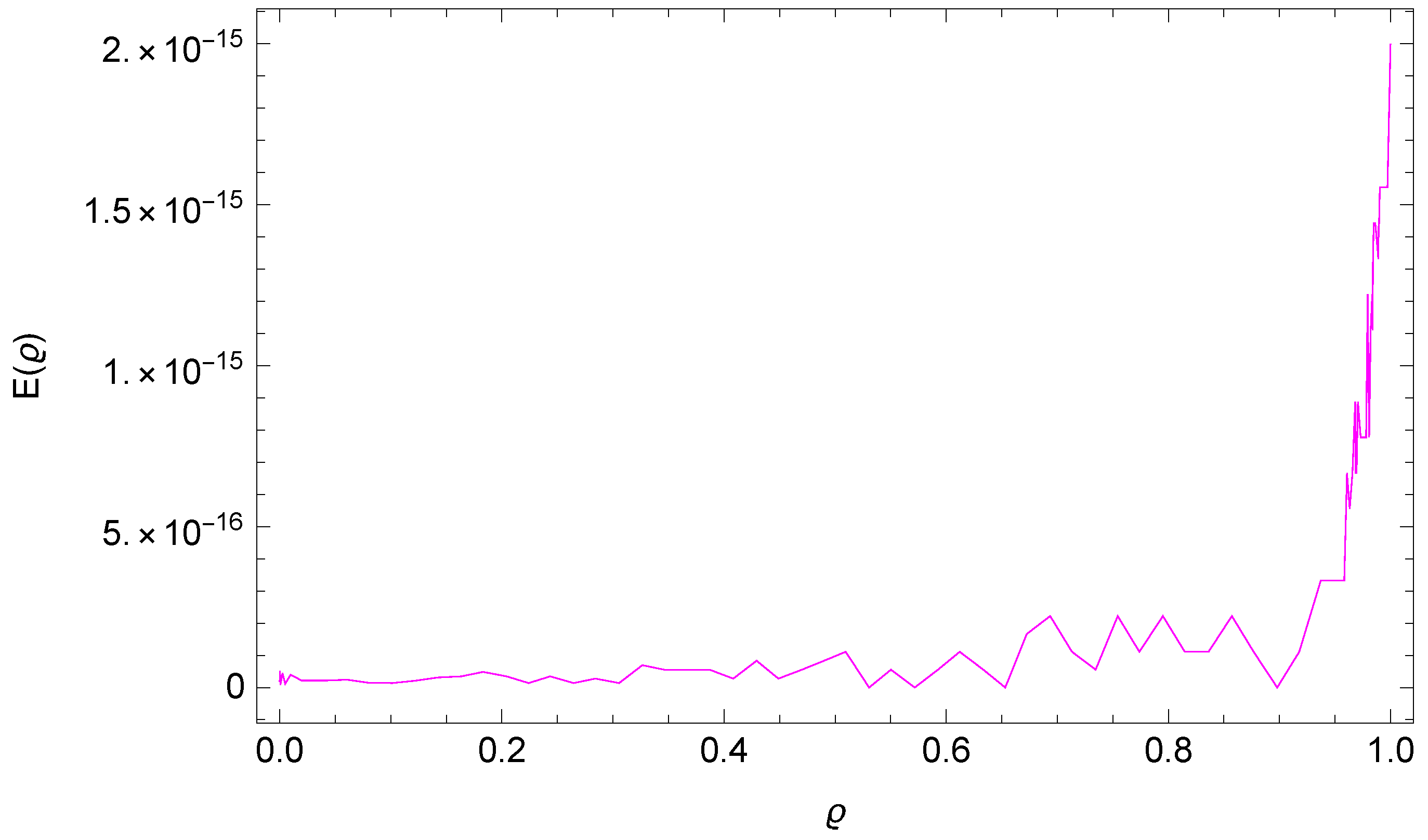
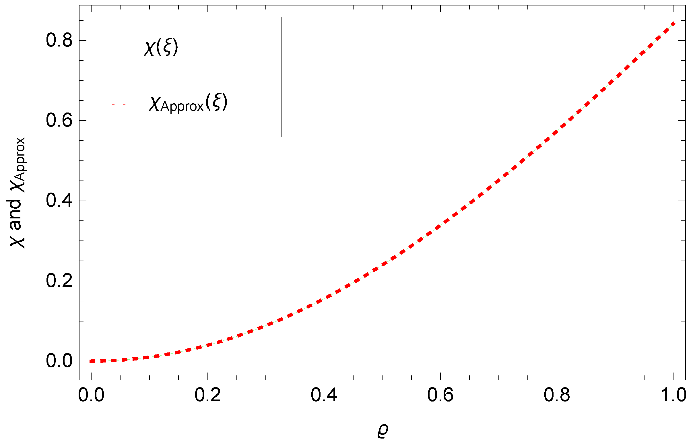
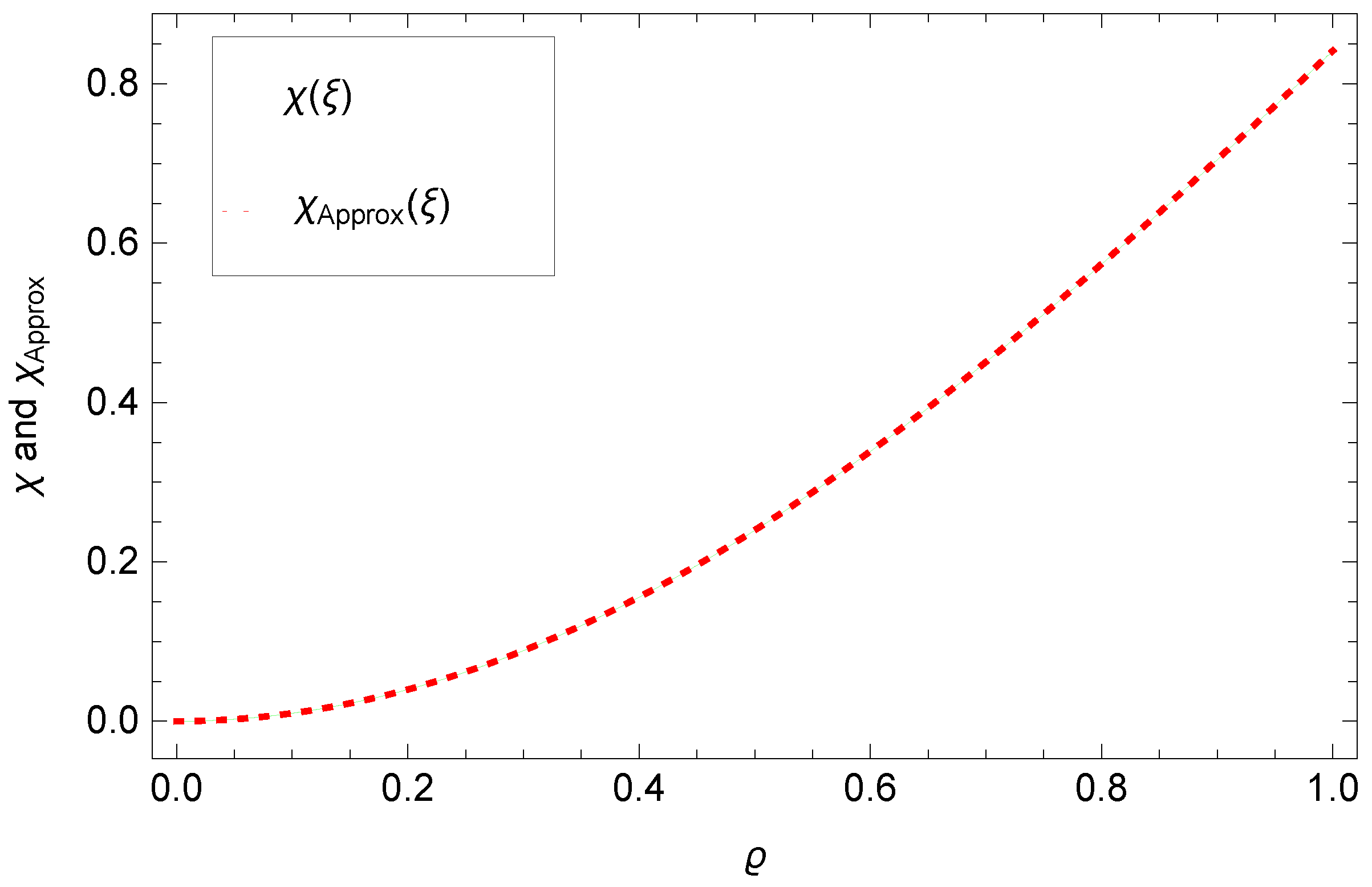
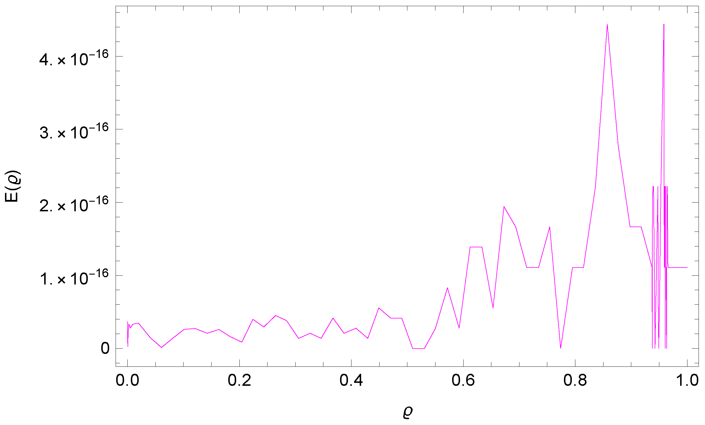
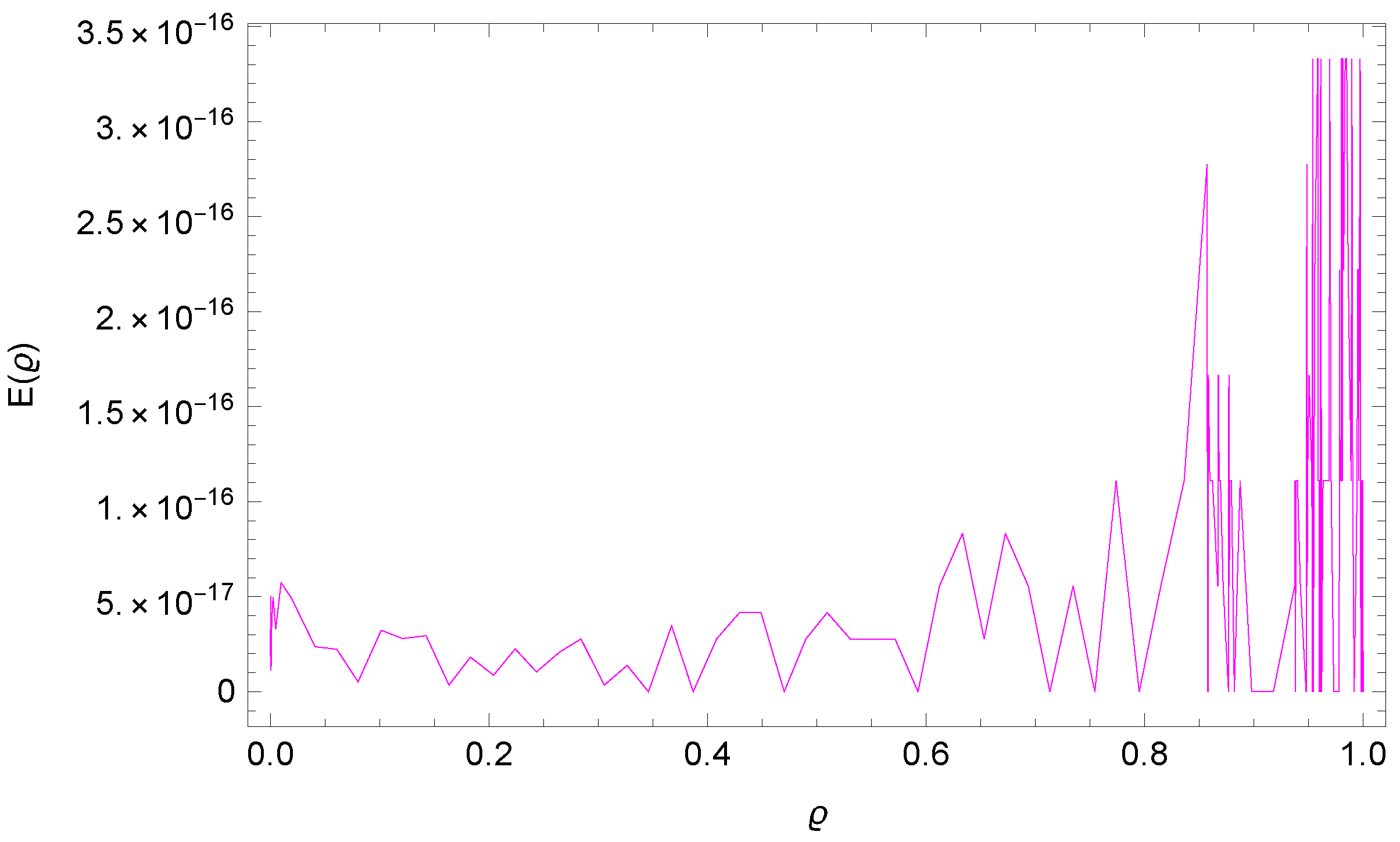
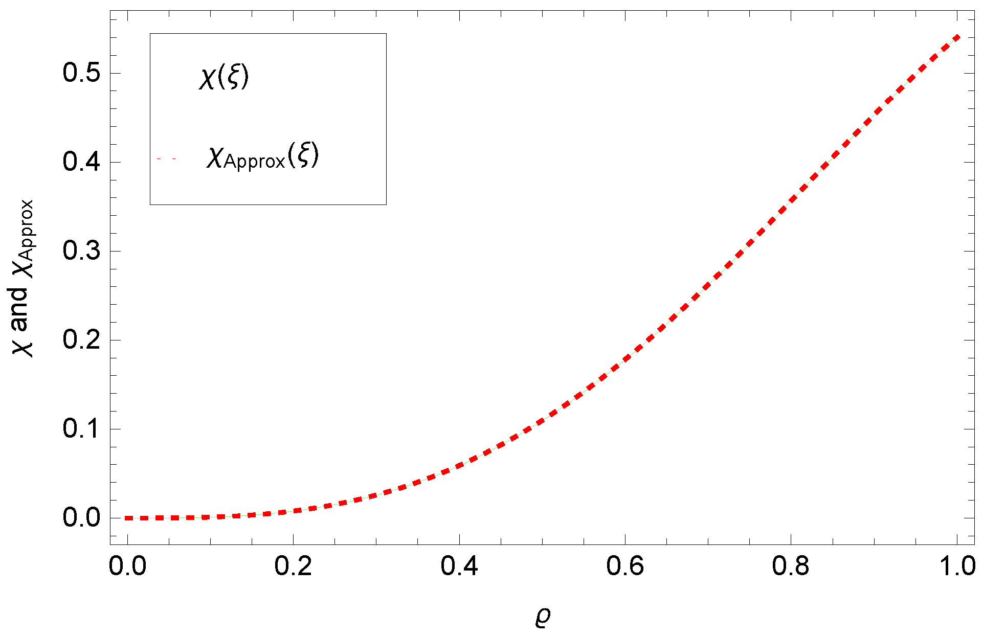
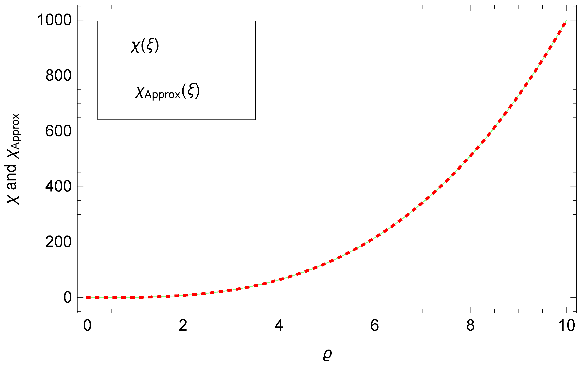
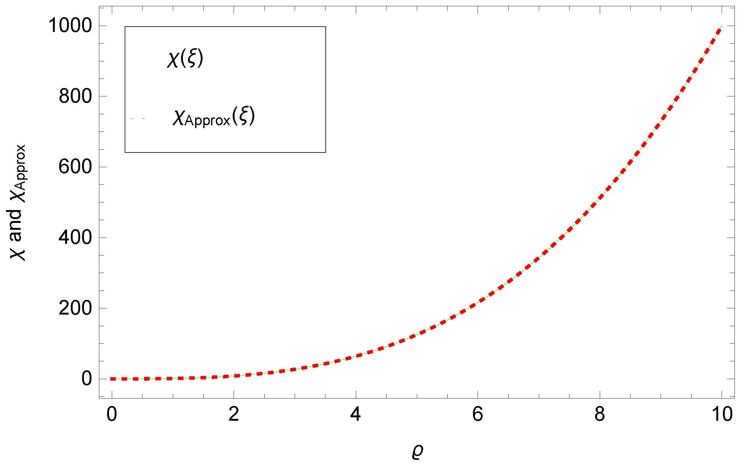
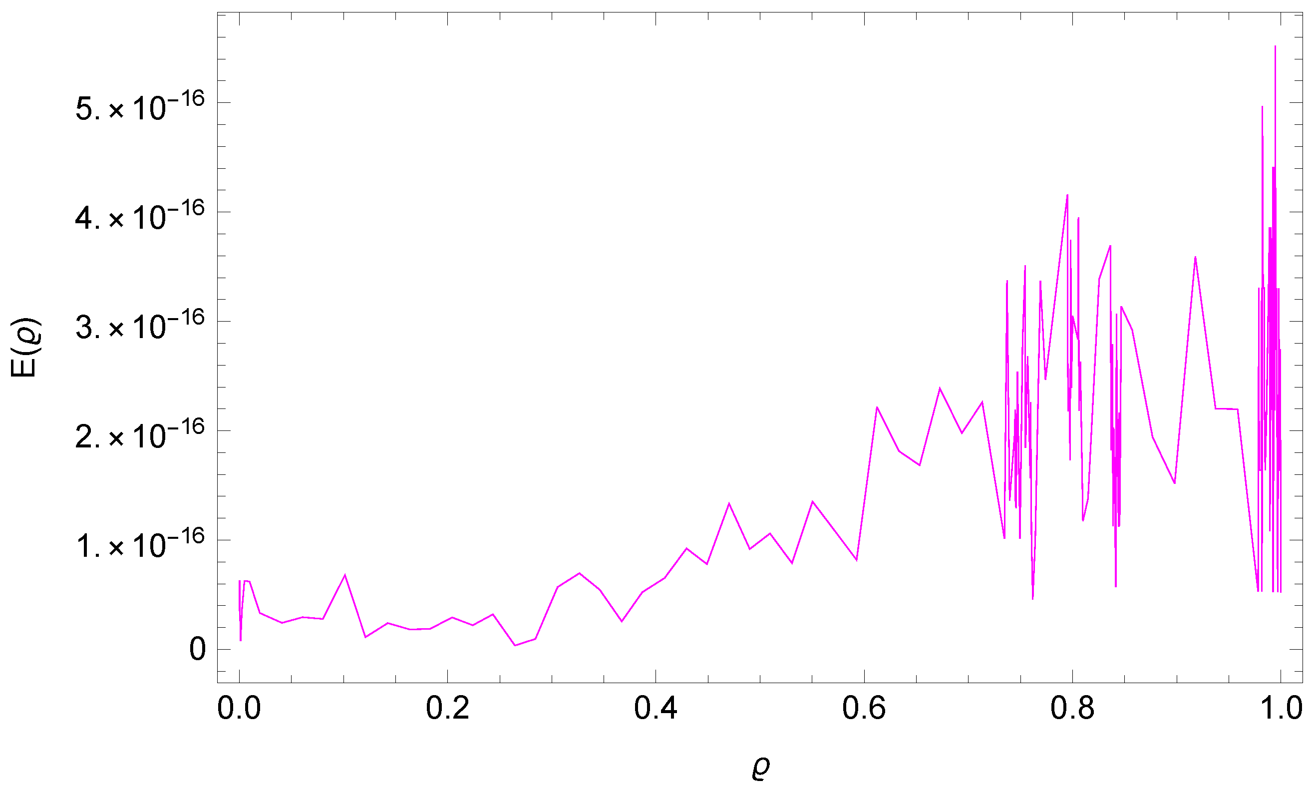
5. Numerical Results

We present several examples to demonstrate the efficacy and power of the proposed technique. Absolute error (AE) is defined as follows:

$$\begin{array}{c}\hfill E\left(\varrho \right)=\mid \mathcal{X}\left(\varrho \right)-{\mathcal{X}}_{Approx}\left(\varrho \right)\mid ,\end{array}$$

(59)

where $\mathcal{X}\left(\varrho \right)$ and ${\mathcal{X}}_{Approx}\left(\varrho \right)$ are the approximate and exact solutions at $\varrho$.

The maximum absolute error (MAE) is defined as:

$$\begin{array}{c}\hfill \mathrm{MAE}=\mathrm{Max}\left\{E\right(\varrho \left)\right\}.\end{array}$$

(60)

Example 1.

We solve the non-linear DO-FBTE with the initial condition:

$$\left\{\begin{array}{c}{D}^2\mathcal{X}\left(\varrho \right)+D\left(\varrho \right)+D^{W\left({\alpha }_1\right)}\mathcal{X}\left(\varrho \right)+{\left(\mathcal{X}\left(\varrho \right)\right)}^2=\eta \left(\varrho \right),\hfill \\ \mathcal{X}\left(0\right)=0,{\mathcal{X}}^{{}^{\prime }}\left(0\right)=0,\hfill \end{array}\right.$$

(61)

where $\eta \left(\varrho \right)$ is the source function such that the exact solution $\mathcal{X}\left(\varrho \right)=\varrho sin\left(\varrho \right)$,

where $D^{W\left({\alpha }_1\right)}\mathcal{X}\left(\varrho \right)={\int }_0^1\Gamma ({\alpha }_1-0.5)D^{{\alpha }_1}\mathcal{X}\left(\varrho \right)d{\alpha }_1$.

Table 1. The MAE of Example 1 for various ${\nu }_1$ and ${\alpha }_1$.

${\mathit{\nu }}_1$	2	6	10	14
${\alpha }_1=0.9$	$3.74\times {10}^{-2}$	$1.68\times {10}^{-6}$	$2.79\times {10}^{-12}$	$9.66\times {10}^{-15}$
${\alpha }_1=1.3$	$4.90\times {10}^{-2}$	$2.10\times {10}^{-6}$	$3.40\times {10}^{-12}$	$6.77\times {10}^{-15}$
${\alpha }_1=1.7$	$6.28\times {10}^{-2}$	$2.56\times {10}^{-6}$	$3.85\times {10}^{-12}$	$1.89\times {10}^{-15}$

presents the MAE with the proposed method at different values of ${\alpha }_1$ and ${\nu }_1$. We can see from the outcomes that the suggested scheme yields superior accuracy. Additionally, it should be noted that good approximations can be made with only a few points. In Figure 2, Figure 3 and Figure 4, we depict the AE values listed in Table 1. Figure 5, Figure 6 and Figure 7 compare the exact and approximate solutions. In Figure 8, we represent the logarithmic of $M_E$ (${log}_{10}{M}_E$) for different values of ${\nu }_1$. Taking ${\nu }_1=14$, we obtain the numerical result of Example 1 as:

$$\begin{array}{cc}\hfill {\mathcal{X}}_{Approx}\left(\varrho \right)& =-2.22045\times {10}^{-16}\varrho +4.22995\times {10}^{-14}{\varrho }^2+{\varrho }^3\hfill \\ & +3.11761\times {10}^{-11}{\varrho }^4-0.5{\varrho }^5+2.12404\times {10}^{-9}{\varrho }^6+0.0416667{\varrho }^7\hfill \\ & +2.91241\times {10}^{-8}{\varrho }^8-0.00138895{\varrho }^9+1.01277\times {10}^{-7}{\varrho }^{10}\hfill \\ & +0.0000246878{\varrho }^{11}+8.90575\times {10}^{-8}{\varrho }^{12}-3.21822\times {10}^{-7}{\varrho }^{13}+1.44304\times {10}^{-8}{\varrho }^{14}\hfill \end{array}$$

(62)

Example 2.

We solve the non-linear DO-FBTE with the boundary conditions:

$$\left\{\begin{array}{c}{D}^2\mathcal{X}\left(\varrho \right)+D\left(\varrho \right)+D^{W\left({\alpha }_1\right)}\mathcal{X}\left(\varrho \right)+{\left(\mathcal{X}\left(\varrho \right)\right)}^3=\eta \left(\varrho \right),\hfill \\ \mathcal{X}\left(0\right)=0,\mathcal{X}\left(1\right)=cos\left(1\right),\hfill \end{array}\right.$$

(63)

where $\eta \left(\varrho \right)$ is the source function such that the exact solution $\mathcal{X}\left(\varrho \right)={\varrho }^{3}cos\left(\varrho \right)$,

where $D^{W\left({\alpha }_1\right)}\mathcal{X}\left(\varrho \right)={\int }_0^1\Gamma ({\alpha }_1-\frac{3}{2})D^{{\alpha }_1}\mathcal{X}\left(\varrho \right)d{\alpha }_1$.

In Figure 9, Figure 10 and Figure 11, we depict the AE values listed in

Table 2. The MAE of Example 2 for various ${\nu }_1$ and ${\alpha }_1$.

${\mathit{\nu }}_1$	2	6	10	14
${\alpha }_1=0.9$	$5.32\times {10}^{-2}$	$6.14\times {10}^{-6}$	$1.42\times {10}^{-11}$	$4.44\times {10}^{-16}$
${\alpha }_1=1.3$	$1.73\times {10}^{-1}$	$1.98\times {10}^{-5}$	$2.44\times {10}^{-11}$	$5.55\times {10}^{-16}$
${\alpha }_1=1.7$	$7.24\times {10}^{-2}$	$6.80\times {10}^{-6}$	$3.85\times {10}^{-12}$	$5.55\times {10}^{-16}$

. Figure 12, Figure 13 and Figure 14 compare the exact and approximate solutions. In Figure 15, we represent the logarithmic of $M_E$ (${log}_{10}{M}_E$) for different values of ${\nu }_1$. Table 2 presents the MAE with the proposed method at different values of ${\alpha }_1$ and ${\nu }_1$. The results show that the proposed strategy produces greater accuracy. It should also be highlighted that good approximations can be made with just a few points.

Taking ${\nu }_1=14$, we obtain the numerical result of Example 2 as:

$$\begin{array}{cc}\hfill {\mathcal{X}}_{Approx}\left(\varrho \right)& ={\varrho }^2-2.13496\times {10}^{-13}{\varrho }^3-0.166667{\varrho }^4-2.40013\times {10}^{-11}{\varrho }^5\hfill \\ & +0.00833333{\varrho }^6-4.72967\times {10}^{-10}{\varrho }^7-0.000198411{\varrho }^8\hfill \\ & -2.21039\times {10}^{-9}{\varrho }^9+2.75855\times {10}^{-6}{\varrho }^{10}-2.46814\times {10}^{-9}{\varrho }^{11}\hfill \\ & -2.36486\times {10}^{-8}{\varrho }^{12}-4.6222\times {10}^{-10}{\varrho }^{13}+2.25142\times {10}^{-10}{\varrho }^{14}\hfill \end{array}$$

(64)

Example 3.

We solve the linear DO-FBTE with the boundary condition [13]:

$$\left\{\begin{array}{c}a{D}^2\mathcal{X}\left(\varrho \right)+bD\left(\varrho \right)+D^{W\left({\alpha }_1\right)}\mathcal{X}\left(\varrho \right)+c\left(\mathcal{X}\left(\varrho \right)\right)=\eta \left(\varrho \right),\hfill \\ \mathcal{X}\left(0\right)=0,\mathcal{X}\left(1\right)=1,\hfill \end{array}\right.$$

(65)

where $\eta \left(\varrho \right)$ is the source function such that the exact solution $\mathcal{X}\left(\varrho \right)={\varrho }^3$,

where $D^{W\left({\alpha }_1\right)}\mathcal{X}\left(\varrho \right)={\int }_0^1\Gamma ({\alpha }_1-\frac{3}{2})D^{{\alpha }_1}\mathcal{X}\left(\varrho \right)d{\alpha }_1$ and $a=b=c=1.$

In Figure 16, Figure 17 and Figure 18 compare the exact and approximate solutions ${\mathcal{X}}_{Approx}\left(\varrho \right)$ and $\mathcal{X}\left(\varrho \right)$ for Example 3 when ${\nu }_1=8$ and ${\alpha }_1=0.9$, ${\alpha }_1=1.3$ and ${\alpha }_1=1.7$, respectively. Figure 19, Figure 20 and Figure 21, we depict the AE values. We compare the present method at ${\nu }_1=8$ and the method in [13] at ${\nu }_1=10$; for this method, it should be noted that good approximations can be made with only a few points.

Taking ${\nu }_1=2$, we obtain the numerical result of Example 3 as:

$$\begin{array}{cc}\hfill {\mathcal{X}}_{Approx}\left(\varrho \right)& =1.28903{\varrho }^2.\hfill \end{array}$$

(66)

Taking ${\nu }_1=3$, we obtain the numerical result (this is nearly equivalent to the exact solution) of Example 3 as:

$$\begin{array}{cc}\hfill {\mathcal{X}}_{Approx}\left(\varrho \right)& =-1.11022\times {10}^{-15}\varrho +6.66134\times {10}^{-16}{\varrho }^2+{\varrho }^3\simeq {\varrho }^3.\hfill \end{array}$$

(67)

6. Conclusions

In this study, we focus on developing a precise and effective numerical method based on the SL-GL collocation method to generate approximations of DO-FBTE solutions. The technique uses shifted fractional Legendre–Gauss collocation points as interpolation nodes and a truncated series of shifted Legendre polynomials to approximate the DO-FBTE solution. Then, the original DO-FBTE is transformed into an algebraic equation system by computing the residuals at the SL-GL quadrature points. The efficiency of the suggested system was verified using a collection of numerical examples. The approach fared better in terms of accuracy than other options.

References

1. Guo, L.; Zhao, X.L.; Gu, X.M.; Zhao, Y.L.; Zheng, Y.B.; Huang, T.Z. Three-dimensional fractional total variation regularized tensor optimized model for image deblurring. Appl. Math. Comput. 2021, 404, 126224. [Google Scholar] [CrossRef]
2. Miller, K.; Ross, B. An Introduction to the Fractional Calculus and Fractional Differential Equations; Wiley: Hoboken, NJ, USA, 1993. [Google Scholar]
3. Ali, H.; Kamrujjaman, M.; Shirin, A. Numerical solution of a fractional-order Bagley–Torvik equation by quadratic finite element method. J. Appl. Math. Comput. 2021, 66, 351–367. [Google Scholar] [CrossRef]
4. Ji, T.; Hou, J. Numerical solution of the Bagley–Torvik equation using Laguerre polynomials. SeMA J. 2020, 77, 97–106. [Google Scholar] [CrossRef]
5. Mohammadi, F.; Mohyud-Din, S. A fractional-order Legendre collocation method for solving the Bagley-Torvik equations. Adv. Differ. Equ. 2016, 2016, 269. [Google Scholar] [CrossRef]
6. Deshi, A.; Gudodagi, G. Numerical solution of Bagley–Torvik, nonlinear and higher order fractional differential equations using Haar wavelet. SeMA J. 2021, 79, 663–675. [Google Scholar] [CrossRef]
7. Izadi, M.; Negar, M. Local discontinuous Galerkin approximations to fractional Bagley-Torvik equation. Math. Methods Appl. Sci. 2020, 43, 4798–4813. [Google Scholar] [CrossRef]
8. Syam, M.; Alsuwaidi, A.; Alneyadi, A.; Al Refai, S.; Al Khaldi, S. An Implicit Hybrid Method for Solving Fractional Bagley-Torvik Boundary Value Problem. Mathematics 2018, 6, 109. [Google Scholar] [CrossRef]
9. Nouri, K.; Elahi-Mehr, S.; Torkzadeh, L. Investigation of the behavior of the fractional Bagley-Torvik and Basset equations via numerical inverse Laplace transform. Rom. Rep. Phys. 2016, 68, 503–514. [Google Scholar]
10. Karaaslan, M.; Celiker, F.; Kurulay, M. Approximate solution of the Bagley–Torvik equation by hybridizable discontinuous Galerkin methods. Appl. Math. Comput. 2016, 285, 51–58. [Google Scholar] [CrossRef]
11. Torvik, P.J.; Bagley, R.L. On the appearance of the fractional derivative in the behavior of real materials. J. Appl. Mech. 1984, 51, 294–298. [Google Scholar] [CrossRef]
12. Morgado, M.; Rebelo, M.; Ferrás, L. Finite Difference Schemes with Non-uniform Time Meshes for Distributed-Order Diffusion Equations. In Proceedings of the International Workshop on Advanced Theory and Applications of Fractional, Calculus, Online, 6–8 September 2021; pp. 239–244. [Google Scholar]
13. Aminikhah, H.; Sheikhani, A.H.R.; Houlari, T.; Rezazadeh, H. Numerical solution of the distributed-order fractional Bagley-Torvik equation. IEEE/CAA J. Autom. Sin. 2017, 6, 760–765. [Google Scholar] [CrossRef]
14. Yuttanan, B.; Razzaghi, M. Legendre wavelets approach for numerical solutions of distributed order fractional differential equations. Appl. Math. Model. 2019, 70, 350–364. [Google Scholar] [CrossRef]
15. Jibenja, N.; Yuttanan, B.; Razzaghi, M. An efficient method for numerical solutions of distributed-order fractional differential equations. J. Comput. Nonlinear Dyn. 2018, 13, 111003. [Google Scholar] [CrossRef]
16. Maleknejad, K.; Rashidinia, J.; Eftekhari, T. Numerical solutions of distributed order fractional differential equations in the time domain using the Müntz–Legendre wavelets approach. Numer. Methods Partial Differ. Equ. 2021, 37, 707–731. [Google Scholar] [CrossRef]
17. Pourbabaee, M.; Saadatmandi, A. Collocation method based on Chebyshev polynomials for solving distributed order fractional differential equations. Comput. Methods Differ. Equ. 2021, 9, 858–873. [Google Scholar]
18. Rashidinia, J.; Eftekhari, T.; Maleknejad, K. A novel operational vector for solving the general form of distributed order fractional differential equations in the time domain based on the second kind Chebyshev wavelets. Numer. Algorithms 2021, 88, 1617–1639. [Google Scholar] [CrossRef]
19. Delzanno, G.L. Multi-dimensional, fully-implicit, spectral method for the Vlasov–Maxwell equations with exact conservation laws in discrete form. J. Comput. Phys. 2015, 301, 338–356. [Google Scholar] [CrossRef]
20. Chen, Y.; Zhou, J. Error estimates of spectral Legendre–Galerkin methods for the fourth-order equation in one dimension. Appl. Math. Comput. 2015, 268, 1217–1226. [Google Scholar] [CrossRef]
21. Abdelkawy, M.; Amin, A.; Lopes, A.M. Fractional-order shifted Legendre collocation method for solving non-linear variable-order fractional Fredholm integro-differential equations. Comput. Appl. Math. 2022, 41, 2. [Google Scholar] [CrossRef]
22. Amin, A.; Abdelkawy, M.; Amin, A.K.; Lopes, A.M.; Alluhaybi, A.A.; Hashim, I. Legendre-Gauss-Lobatto collocation method for solving multi-dimensional systems of mixed Volterra-Fredholm integral equations. AIMS Math. 2023, 8, 20871–20891. [Google Scholar] [CrossRef]
23. Ezz-Eldien, S.S. On solving systems of multi-pantograph equations via spectral tau method. Appl. Math. Comput. 2018, 321, 63–73. [Google Scholar] [CrossRef]
24. Hafez, R.M.; Hammad, M.; Doha, E.H. Fractional Jacobi Galerkin spectral schemes for multi-dimensional time fractional advection–diffusion–reaction equations. Eng. Comput. 2022, 38, 841–858. [Google Scholar] [CrossRef]
25. Hammad, M.; Hafez, R.M.; Youssri, Y.H.; Doha, E.H. Exponential Jacobi-Galerkin method and its applications to multidimensional problems in unbounded domains. Appl. Numer. Math. 2020, 157, 88–109. [Google Scholar] [CrossRef]
26. Abdelkawy, M.; Alyami, S. Legendre-Chebyshev spectral collocation method for two-dimensional nonlinear reaction-diffusion equation with Riesz space-fractional. Chaos Solitons Fractals 2021, 151, 111279. [Google Scholar] [CrossRef]
27. Amin, A.; Amin, A.; Abdelkawy, M.; Alluhaybi, A.; Hashim, I. Spectral technique with convergence analysis for solving one and two-dimensional mixed Volterra-Fredholm integral equation. PLoS ONE 2023, 18, e0283746. [Google Scholar] [CrossRef]
28. Doha, E.; Abdelkawy, M.; Amin, A.; Lopes, A. On spectral methods for solving variable-order fractional integro-differential equations. Comput. Appl. Math. 2018, 37, 3937–3950. [Google Scholar] [CrossRef]
29. Shen, J.; Tang, T.; Wang, L. Spectral Methods: Algorithms, Analysis and Applications; Springer: Berlin/Heidelberg, Germany, 2011; Volume 41. [Google Scholar]
30. Canuto, C.; Hussaini, M.Y.; Quarteroni, A.; Zang, T.A. Spectral Methods: Fundamentals in Single Domains; Springer: Berlin/Heidelberg, Germany, 2007. [Google Scholar]
31. Amin, A.Z.; Lopes, A.M.; Hashim, I. A Chebyshev collocation method for solving the non-linear variable-order fractional Bagley–Torvik differential equation. Int. J. Nonlinear Sci. Numer. Simul. 2022, 24, 5. [Google Scholar] [CrossRef]
32. Bhrawy, A.; Doha, E.; Alzaidy, J.; Abdelkawy, M. A space-time spectral collocation algorithm for the variable order fractional wave equation. SpringerPlus 2016, 5, 1220. [Google Scholar] [CrossRef]
33. Chen, F.; Shen, J. Efficient spectral-Galerkin methods for systems of coupled second-order equations and their applications. J. Comput. Phys. 2012, 231, 5016–5028. [Google Scholar] [CrossRef]
34. Yang, Y. Jacobi spectral Galerkin methods for fractional integro-differential equations. Calcolo 2015, 52, 519–542. [Google Scholar] [CrossRef]
Figure 1. Flowchart of our methodology.
Fractalfract 07 00780 g001
Figure 2. The AE for Example 1 when ν 1 = 14 and α 1 = 0.9 .
Fractalfract 07 00780 g002
Figure 3. The AE for Example 1 when ν 1 = 14 and α 1 = 1.3 .
Fractalfract 07 00780 g003
Figure 4. The AE for Example 1 when ν 1 = 14 and α 1 = 1.7 .
Fractalfract 07 00780 g004
Figure 5. The X A p p r o x ( ϱ ) and X ( ϱ ) for Example 1 when ν = 14 and α 1 = 0.9 .
Fractalfract 07 00780 g005
Figure 6. The X A p p r o x ( ϱ ) and X ( ϱ ) for Example 1 when ν = 14 and α 1 = 1.3 .
Fractalfract 07 00780 g006
Figure 7. The X A p p r o x ( ϱ ) and X ( ϱ ) for Example 1 when ν = 14 and α 1 = 1.7 .
Fractalfract 07 00780 g007
Figure 8. The M E convergence for Example 1 when α 1 = 0.9 and α 1 = 1.7 .
Fractalfract 07 00780 g008
Figure 9. The AE for Example 2 when ν 1 = 14 and α 1 = 0.9 .
Fractalfract 07 00780 g009
Figure 10. The AE for Example 2 when ν 1 = 14 and α 1 = 1.3 .
Fractalfract 07 00780 g010
Figure 11. The AE for Example 2 when ν 1 = 14 and α 1 = 1.7 .
Fractalfract 07 00780 g011
Figure 12. The X A p p r o x ( ϱ ) and X ( ϱ ) for Example 2 when ν = 14 and α 1 = 0.9 .
Fractalfract 07 00780 g012
Figure 13. The X A p p r o x ( ϱ ) and X ( ϱ ) for Example 2 when ν = 14 and α 1 = 1.3 .
Fractalfract 07 00780 g013
Figure 14. The X A p p r o x ( ϱ ) and X ( ϱ ) for Example 2 when ν = 14 and α 1 = 1.7 .
Fractalfract 07 00780 g014
Figure 15. The M E convergence for Example 2 when α 1 = 0.9 , α 1 = 1.3 and α 1 = 1.7 .
Fractalfract 07 00780 g015
Figure 16. The X A p p r o x ( ϱ ) and X ( ϱ ) for Example 3 when ν = 8 and α 1 = 0.9 .
Fractalfract 07 00780 g016
Figure 17. The X A p p r o x ( ϱ ) and X ( ϱ ) for Example 3 when ν = 8 and α 1 = 1.3 .
Fractalfract 07 00780 g017
Figure 18. The X A p p r o x ( ϱ ) and X ( ϱ ) for Example 3 when ν = 8 and α 1 = 1.7 .
Fractalfract 07 00780 g018
Figure 19. The AE for Example 3 when ν 1 = 8 and α 1 = 0.9 .
Fractalfract 07 00780 g019
Figure 20. The AE for Example 3 when ν 1 = 8 and α 1 = 1.3 .
Fractalfract 07 00780 g020
Figure 21. The AE for Example 3 when ν 1 = 8 and α 1 = 0.9 .
Fractalfract 07 00780 g021