Abstract
This study investigates the pricing formula for European options when the underlying asset follows a fuzzy mixed weighted fractional Brownian motion within a jump environment. We construct a pricing model for European options driven by fuzzy mixed weighted fractional Brownian motion with jumps. By converting the partial differential equation (PDE) into a Cauchy problem, we derive explicit solutions for both European call options and European put options. The figures and tables demonstrating the effectiveness of the results highlight the suitability of the fuzzy mixed weighted fractional Brownian motion with jump model for option pricing.
1. Introduction
Since Black and Scholes [1] proposed the Black–Scholes model in 1973, a pioneering development of an option pricing model, the modern theory of option pricing has undergone rapid advancement. However, the assumptions within the Black–Scholes model, namely the geometric Brownian motion of the underlying asset price and constant volatility, fail to conform to the realities of financial markets. Consequently, substantial disparities between the theoretical prices calculated using the Black–Scholes model and actual market prices have emerged. As a result, scholars have undertaken efforts to enhance and expand the Black–Scholes model, as evidenced in scholarly works [2,3,4], where researchers have proposed the utilization of fractional Brownian motion (fBm in short) models exhibiting long-memory features as an enhancement to the classical Black–Scholes model.
Fractional Brownian motion represents a self-similar Gaussian process with stationary increments, characterized by the Hurst parameter H. The value of this parameter determines the degree of long-term dependence within the process. Recently, Mehrdoust and Najafi [5] succeeded in deducing explicit solutions for the fractional Black–Scholes model, characterized by a somewhat less resilient payoff function. Although fBm could effectively encompass the extended correlations among returns spanning different days, Rogers [6] showcased that it concurrently introduced the potential for arbitrage opportunities. To address this challenge and accommodate the enduring memory characteristic, EI-Nouty [7] and Mishura [8] illustrated the feasibility of employing a mixed fractional Brownian motion (mfBm in short), thereby capturing the intermittent variations in financial assets. Moreover, Cheridito [9] established the equivalence between the mfBm and a Brownian motion under the condition of the Hurst exponent . This mathematical equivalence removes the potential for arbitrage, enabling valid financial use. For more applications of mfBm on financial models, please refer to [10,11,12]. Recently, another type of fractional Gaussian process–sub-fractional Brownian motion was also used in applications for option pricing, as seen in [13,14,15]. For example, Guo et al. [15] studied the issue of time-varying implied volatility of options and applied its model to option pricing under sub-mixed fractional Brownian motion. The article concluded, through comparative analysis of four models, namely Brownian motion, fractional Brownian motion, sub-fractional Brownian motion, and sub-mixed fractional Brownian motion, that the model of sub-mixed fractional Brownian motion exhibited the best pricing performance.
Bojedcki et al. [16] proposed an extension to fractional Brownian motion called weighted fractional Brownian motion (weighted-fBm in short). This extension incorporates a weighting function and exhibits non-stationary increments, thus offering a more flexible dependency structure. From this vantage point, the model of weighted-fBm might be better suited for capturing the behavior of financial systems. In such systems, investors often delay decisions until information surpasses a particular threshold. Nevertheless, according to the literature [17], it can be understood that the pricing model of the underlying asset driven by a fractional Gaussian process may lead to arbitrage opportunities. To avoid this issue, the commonly employed method is to construct a linear combination of a standard Brownian motion and a fractional Gaussian process (for example, a fractional Brownian motion or a sub-fractional Brownian motion), as described in [9,10,11,12,13,14,15], among others. This research also adopts such an approach, constructing a mixture of standard Brownian motion and weighted-fBm as a linear combination. Khalaf et al. [18] pointed out that this mixture, along with the asymptotic stationary properties for weighted-fBm, opened up the possibility of the mixture being a martingale or equivalent to Brownian motion, as it is the same as mfBm. This indicates that the pricing model of the underlying asset driven by a mixed weighted fractional Brownian motion is arbitrage-free.
Furthermore, the uncertainty in financial markets stems not only from stochasticity but also ambiguity. In practice, recorded financial data contain inaccuracies, especially for risk-free rates and volatility. For instance, the risk-free rate used in pricing European options is only an approximation, since different institutions have varying rates. Zadeh [19] pioneered fuzzy set theory in 1965, providing a key technique for modeling ambiguous markets. Wu [20] then incorporated fuzzy sets into option pricing, proposing fuzzy pricing models for European options. Fuzzy set theory can be employed to quantify uncertainty and risk, facilitating a more comprehensive assessment of option prices. By introducing fuzzy random variables, the impact of various factors on option prices can be considered, contributing to a more accurate reflection of market uncertainty. In this study, the triangular fuzzy number is introduced for the estimation of relevant parameters. The choice of employing the triangular fuzzy number is based on their relatively simple representation and form, making them more easily interpretable and understandable. The triangular fuzzy number offers an intuitive grasp of the boundaries and central tendencies of a fuzzy set.
Recently, Zhang et al. [21] discussed the pricing problem of European options under the assumption that the underlying stock price, the risk-free interest rate, the volatility, the jump intensity, and the mean value and variance of jump magnitudes are all fuzzy numbers. Bian and Li [22] used stochastic analysis, fractal theory, and fuzzy set theory to construct a European option pricing model based on the long-term memory property of the financial market in an uncertain environment, and the conclusions showed that the European option pricing model with long-term memory property was more suitable for financial markets in an uncertain environment. More related studies can be referred to in [23,24,25]. To tackle these challenges, we propose a new framework for pricing European options under a fuzzy mixed weighted-fBm model with jumps. This flexible model incorporates both mixed weighted-fBm to capture long-range dependence and jumps to represent sudden price changes, while using fuzzy sets to model inherent data uncertainty. By capturing a wider range of asset price behaviors, our approach is similar to the treatment of [21] in enhancing the accuracy of options pricing.
The subsequent sections of this paper are structured as follows: Section 2 expounds on the mixed weighted-fBm and fuzzy set theory, providing essential preliminary knowledge. In Section 3, we derive the corresponding It’sformula for the asset price propelled by the mixed weighted-fBm with jumps, and provide the expressions for the underlying asset price. In Section 4, we acquire the Black–Scholes partial differential equation along with the solution in a closed-form for European options. In Section 5, we present a fuzzy stochastic process that employs fuzzy random variables to define the underlying asset price process, and deduce the -cut of the fuzzy price of European options. Section 6 presents numerical results using European call options. The findings demonstrate the sensitivity of the fuzzy option prices to changes in b and . Section 7 provides a conclusion.
2. Preliminaries
Let be a complete probability space, endowed with a filtration that adheres faithfully to the usual conditions.
2.1. Mixed Weighted-fBm
Definition 1.
The mixed weighted-fBm is a linear combination of the Brownian motion and the weighted-fBm , which can be expressed as
where are the index and satisfy the condition . are positive constants; and are independent of each other. is defined by [26].
In what follows, we present certain attributes of the mixed weighted-fBm through the proposition delineated hereafter. For more detailed information about the properties of the mixed weighted-fBm, one can refer to [18,26].
Proposition 1.
where , and is the beta function.
The mixed weighted-fBm has the following properties:
- is a central Gaussian process.
- When , .
- , the covariance of and is
2.2. Fuzzy Set Theory
Definition 2
(Fuzzy number [20]). represents a fuzzy subset of the set of real numbers, denoted by R. earns the appellation of a fuzzy number under the following conditions:
- (1)
- qualifies as both a normal fuzzy set and a convex fuzzy set;
- (2)
- The membership function of exhibits upper semi-continuity;
- (3)
- The α-level set of remains confined within boundaries.
If is a fuzzy number, its -cut set is a bounded closed interval. We can denote . When , then we have .
Definition 3
(Triangle fuzzy number [27]). Allow to denote a veritable fuzzy set within the realm of Group R, and it earns the distinguished title of a triangular fuzzy number when its membership function is meticulously defined as such:
The utmost despondent extent of uncertainty, denoted as , is embodied by , while the zenith of optimism is marked by , and at the heart of it all lies , symbolizing the most probable value. The -cut of manifests itself as a sealed interval, elegantly articulated as follows:
where
3. Asset Pricing Model
In this research, we embrace the venerable theory of financial stochastic analysis, weaving extensions into the fabric of the Black–Scholes model. Moreover, the ensuing suppositions endure as follows:
- (i)
- The temporality of transactions and the magnitude of assets persist in a seamless continuum;
- (ii)
- Transaction expenses and fiscal levies remain conspicuously absent from the equation;
- (iii)
- The dealing involving assets faces no constriction, allowing for both short selling and short buying without hindrance;
- (iv)
- The return of risk-free assets in time period t iswhere constant r is the risk-free interest rate;
- (v)
- The risk assets (stocks) price is driven by the mixed weighted-fBm with jumps:where is the instantaneous expected return of the stock; , and represent the volatility of stock prices; and is a compensated Poisson process with intensity . , and are independent of each other.
Theorem 1.
Let us postulate that takes the form of with an initial value of zero, while exhibits second-order differentiability. Consequently, It ’s formula for the mixed weighted fractional Brownian motion with jumps can be elegantly articulated as such:
Proof.
By virtue of It’s formula for weighted fractional Brownian motion (Refer to Theorem 2.1 in Reference [26] for details) and the analytical technique pertaining to the jump process [28], we derive the following:
The following identities are used by
and is the continuous part of .
Assuming that exhibits second-order differentiability, and considering the Poisson process with intensity , which possesses second-order moment increments, we can invoke a generalized It ’s formula to assert
Combining , we obtain
This completes the proof. □
Theorem 2.
The stock price, which complies with Equation (2), unveils an explicit solution as follows:
4. Pricing Formula for European Option under the Mixed Weight-fBm Model with Jump
Equipped with the unequivocal solution for the stock price , in this section, we shall derive the pricing formula for European call and put options.
Theorem 3.
Supposing that the price of the underlying asset, , adheres to Equation (2), then the value of the contingent claim, denoted as , complies with the ensuing partial differential equation:
Proof.
Using the self-financing strategy , we maintain a number of bonds and stocks to construct the wealth process, the value of which at time t is
Similarly, applying Theorems 1 and 2 gives
where
From Equation (6), we obtain
This completes the proof. □
Theorem 4.
With the underlying asset price following Equation (2), the price at time t of a European call option with strike price K and maturity T is
where
and denotes the standard normal cumulative distribution function.
Proof.
The valuation of the European call option adheres to the ensuing differential equation
Through the utilization of variable substitution, Equation (12) metamorphoses into a Cauchy problem. Let and ; then, .
By substituting the above formula into Equation (12), it can be obtained that
Let
Then, we have
By substituting the above formula into Equation (13), it can be obtained that
In accordance with the classical principles of thermal dynamics, there exists a unique strong solution
Then,
For , let ; we have . Then,
Similarly, for , let ; we have .
Remark 1.
The relationship of parity between the prices of European call option and European put option is expressed as is , which enables us to determine the price of a European put option at time t.
Remark 2.
If , let , then the mixed weighted-fBm with the jump model reduces to the mfBm Black–Scholes model with the Hurst index H, which is consistent with the result in [29,30].
5. European Option Pricing in a Fuzzy Framework
According to Theorem 4 and reference [31], we can readily attain the subsequent findings regarding the fuzzy price, denoted as , of the European call option.
Theorem 5.
With fuzzy interest rate , fuzzy volatility and , fuzzy jump intensity , and fuzzy stock price , the fuzzy European call price at time t is
where
Remark 3.
The relationship of parity between the prices of European call option and European put option is expressed as , which enables us to determine the price of a European put option at time t.
Theorem 6.
The respective interval endpoints of the α-cut for the price of a European call option are
Proof.
The -cut set of can be articulated as .
With regard to the -cut set of fuzzy variables encompassing fuzzy interest rate , fuzzy volatility and , as well as the fuzzy jump intensity , the fuzzy stock price can be delineated as follows: , , , , , .
It can be seen from Equation (11) that
, , , and .
One may ascertain that f is indeed an ascending function with respect to , and . Consequently, the theorem stands as duly established.
This completes the proof. □
The triangle fuzzy number is commonly used to represent fuzzy variables. In this study, the fuzzy interest rate, fuzzy volatility, fuzzy jump intensity, and fuzzy stock price are all modeled as triangle fuzzy numbers to capture their inherent uncertainty. There is , , , , , and . From Definition 3, we can obtain that
;
;
;
;
;
Theorem 7.
When representing the interest rate, volatility, jump intensity, and stock price as triangular fuzzy numbers, the α-cut set for the fuzzy European call price is characterized by its interval endpoints :
where
6. Numerical Experiments
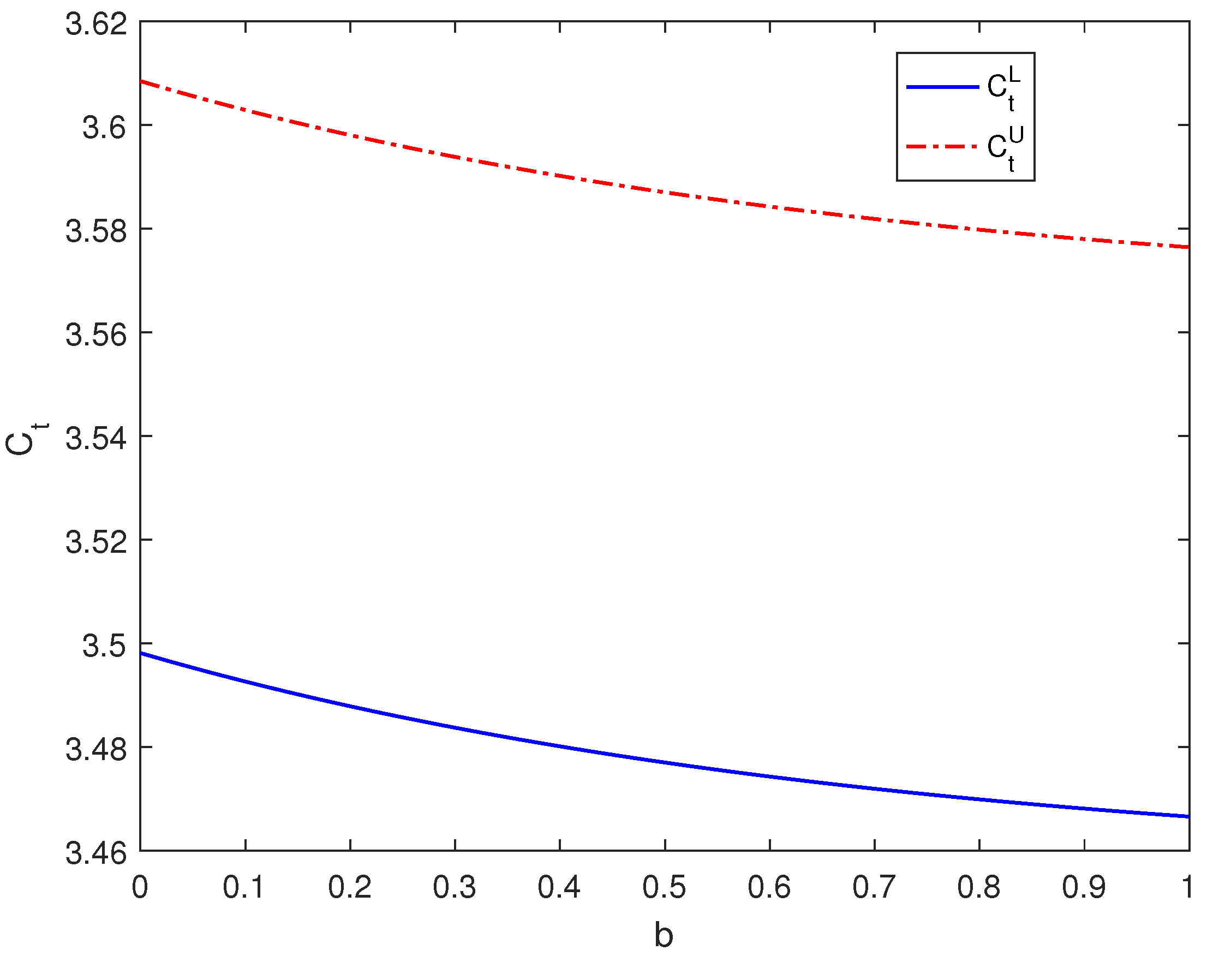
This section thoroughly investigates how the parameter b affects the pricing model by utilizing the control variable method. It provides an exhaustive examination of the sensitivity and stability of the European option pricing model, particularly considering its enduring memory characteristics amidst the backdrop of uncertainty. For simplicity, the numerical experiments use European call option pricing as an example, with European put options following analogous arguments. The parameter values match the benchmark model in Table 1. and represent, respectively, the upper and lower boundaries of European call option prices, and their associated connections can be expressed as follows: , .

Table 1.
Values of benchmark parameters.
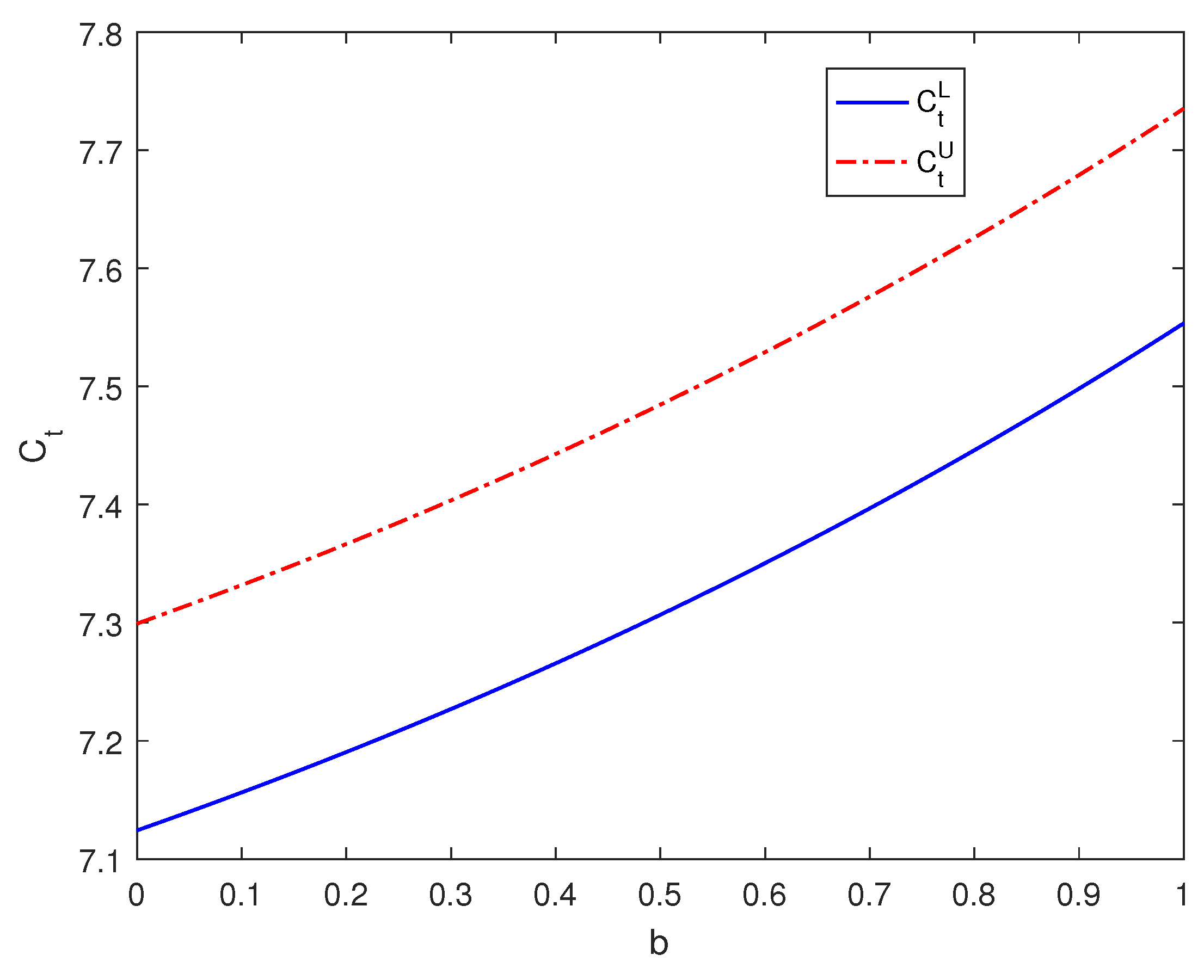
As depicted in Figure 1 and Figure 2, we observe that when the maturity date is set at , the triangular fuzzy price of European call options experiences a decline as parameter b increases. When the maturity date is set at , the triangular fuzzy price of European call options experiences an increase as parameter b increases. By combining the results obtained from Table 2, we can draw the following conclusions: in the range where , an increase in parameter b leads to a reduction in the triangular fuzzy price intervals of European call options. Conversely, in cases where , an increase in parameter b results in an expansion of the triangular fuzzy price intervals of European call options.
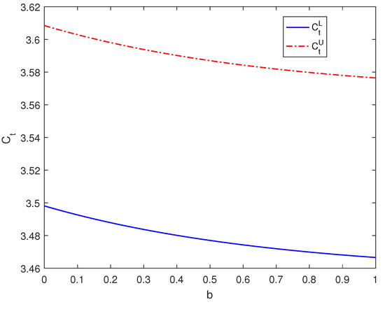
Figure 1.
The impact of parameter b on the pricing of European call options when .
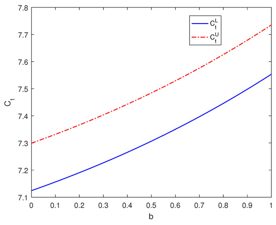
Figure 2.
The impact of parameter b on the pricing of European call options when .
Table 2.
The interval of triangular fuzzy price -cut set for European call option varies across different values of b .
Finally, we compare the proposed pricing model to a model based on weighted fractional Brownian motion (WFBM in short). For simplicity, we ignore jumps and focus on the mixed weighted fractional Brownian motion (MWFBM in short) case. Figure 3 and Figure 4 illustrate how the fuzzy price varies with the parameters b and . The MWFBM model yields higher option prices compared with the WFBM model. Table 3 presents the -cut set intervals of the fuzzy European call price under the two models for different confidence levels . As shown in Table 3, the MWFBM intervals are greater than the WFBM ones. With the current model excluding jumps, if a confidence level of 0.97 is acceptable, any price between 6.7212 and 6.8011 can be chosen. In the event that the market value descends below 6.7212, the individual responsible for making choices regards the price as being undervalued and may opt for the acquisition of the option. Conversely, if the market price surpasses 6.8011, the decision-maker views the price as overvalued and may decide to exercise the option.
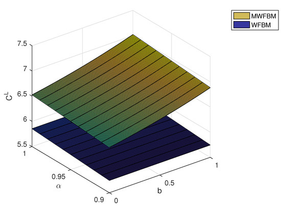
Figure 3.
The values of for both models evolve alongside variations in b and .
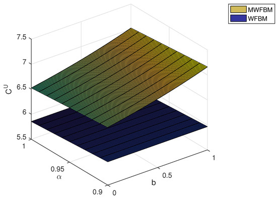
Figure 4.
The values of for both models evolve alongside variations in b and .
Table 3.
A comprehensive analysis of the -cut set intervals of the fuzzy price of European call options under various models.
7. Conclusions
In this research, a fuzzy pricing model for European options is constructed within the framework of mixed weighted fractional Brownian motion with jumps. Using a self-financing strategy, we establish a partial differential equation (PDE) akin to the Black–Scholes model to assess these financial derivatives. We then obtain European option values by applying transform techniques. Similarly, put–call parity holds for the European options. Section 6 presents numerical experiments using European call options. The results demonstrate the sensitivity of fuzzy option prices to b and . Additionally, the MWFBM model is compared with the WFBM model. The results indicate that, for investors, the MWFBM model carries less risk compared with the WFBM model. Based on the conclusions drawn in this study, the next steps in planned research questions and directions include the following:
(i) Improvement of Fuzzy random variables. Despite the advantages of triangular fuzzy number in terms of simplicity and ease of interpretation, their limitation lies in the potential inability to accurately depict some more complex fuzzy set distributions. Future considerations may involve exploring more intricate forms of fuzzy numbers, such as trapezoidal fuzzy numbers or generalized fuzzy number forms, to better capture the characteristics of fuzziness.
(ii) Empirical applications. On the one hand, there is potential to apply the mixed weighted fractional Brownian motion with the jumps model proposed in this paper to other more complex option types, such as Asian options, barrier options, and compound options. On the other hand, empirical simulations could involve comparing the MWFBM model with other long-memory models, such as MFBM (Mixed Fractional Brownian Motion) and MSFBM (Mixed Sub-fractional Brownian Motion), analyzing the accuracy of various models in simulating real financial market conditions.
Author Contributions
Conceptualization, F.X.; methodology, F.X.; software, F.X.; validation, F.X. and X.-J.Y.; formal analysis, F.X.; investigation, F.X.; resources, F.X.; data curation, F.X.; writing—original draft preparation, F.X.; writing—review and editing, X.-J.Y.; visualization, F.X.; supervision, X.-J.Y.; project administration, F.X.; funding acquisition, F.X. All authors have read and agreed to the published version of the manuscript.
Funding
This research was funded by the General Project of Philosophy and Social Science Research in Colleges and Universities of Jiangsu Province (Grant number: 2022SJYB1626).
Data Availability Statement
No new data were created or analyzed in this study. Data sharing is not applicable to this article.
Acknowledgments
We are very grateful to the reviewers for their valuable comments.
Conflicts of Interest
The authors declare no conflict of interest.
Correction Statement
This article has been republished with a minor correction to the Author Contributions. This change does not affect the scientific content of the article.
References
- Black, F.; Scholes, M. The pricing of option and corporate liabilities. J. Polit. Econ. 1973, 81, 637–654. [Google Scholar] [CrossRef]
- Peters, E.E. Fractal structure in the capital market. Financ. Anal. J. 1989, 45, 434–453. [Google Scholar] [CrossRef]
- Hu, Y.; Øksendal, B. Fractional white noise calculus and applications to finance. Infin. Dimens. Anal. Qu. 2003, 6, 1–32. [Google Scholar] [CrossRef]
- Necula, C. Option pricing in a fractional Brownian motion environment. Math. Rep. 2004, 6, 259–273. [Google Scholar] [CrossRef]
- Mehrdoust, F.; Najafi, A.R. Pricing European options under fractional Black-Scholes model with a weak payoff function. Comput. Econ. 2018, 52, 685–706. [Google Scholar] [CrossRef]
- Rogers, L.C.G. Arbitrage with fractional Brownian motion. Math. Financ. 1997, 7, 95–105. [Google Scholar] [CrossRef]
- EI-Nouty, C. The fractional mixed fractional Brownian motion. Stat. Probabil. Lett. 2003, 625, 111–120. [Google Scholar] [CrossRef]
- Mishura, Y.S. Stochastic Calculus for Fractional Brownian Motion and Related Processes; Springer Press: Berlin, Germany, 2008. [Google Scholar]
- Cheridito, P. Mixed fractional Brownian motion. Bernoulli 2001, 7, 913–934. [Google Scholar] [CrossRef]
- Prakasa Rao, B.L.S. Pricing geometric Asian power options under mixed fractional Brownian motion environment. Phys. A 2016, 446, 92–99. [Google Scholar] [CrossRef]
- Shokrollahi, F.; Kılıçman, A. Actuarial approach in a mixed fractional Brownian motion with jumps environment for pricing currency option. Adv. Differ. Equ. 2015, 2015, 257. [Google Scholar] [CrossRef]
- Zhang, W.G.; Li, Z.; Liu, Y.J. Analytical pricing of geometric Asian power options on an underlying driven by a mixed fractional Brownian motion. Phys. A 2018, 490, 402–418. [Google Scholar] [CrossRef]
- Xu, F.; Zhou, S. Pricing of perpetual American put option with sub-mixed fractional Brownian motion. Fract. Calc. Appl. Anal. 2019, 22, 1145–1154. [Google Scholar] [CrossRef]
- Wang, X.; Wang, J.; Guo, Z. Pricing equity warrants under the sub-mixed fractional Brownian motion regime with stochastic interest rate. AIMS Math. 2022, 7, 16612–16631. [Google Scholar] [CrossRef]
- Guo, J.; Kang, W.; Wang, Y. Option pricing under sub-mixed fractional Brownian motion based on time-varying implied volatility using intelligent algorithms. Soft Comput. 2023, 27, 15225–15246. [Google Scholar] [CrossRef]
- Bojdecki, T.; Gorostiza, L.; Talarczyk, A. Occupation time limits of inhomogeneous Poisson systems of independent particles. Stoch. Proc. Appl. 2008, 118, 28–52. [Google Scholar] [CrossRef]
- Zhang, X.; Xiao, W. Arbitrage with fractional Gaussian processes. Phys. A 2017, 471, 620–628. [Google Scholar] [CrossRef]
- Khalaf, A.D.; Zeb, A.; Saeed, T.; Abouagwa, M.; Djilali, S.; Alshehri, H.M. A Special Study of the Mixed Weighted Fractional Brownian Motion. Fractal Fract. 2021, 5, 192. [Google Scholar] [CrossRef]
- Zadeh, L.A. Fuzzy sets, information and control. Inf. Control 2001, 8, 338–353. [Google Scholar] [CrossRef]
- Wu, H.C. Using fuzzy sets theory and Black-Scholes formula to generate pricing boundaries of European options. Appl. Math. Comput. 2007, 185, 136–146. [Google Scholar] [CrossRef]
- Zhang, W.G.; Li, Z.; Liu, Y.J.; Zhang, Y. Pricing European Option Under Fuzzy Mixed Fractional Brownian Motion Model with Jumps. Comput. Econ. 2021, 58, 483–515. [Google Scholar] [CrossRef]
- Bian, L.; Li, Z. Fuzzy simulation of European option pricing using sub-fractional Brownian motion. Chaos Solitons Fractals 2021, 153, 111442. [Google Scholar] [CrossRef]
- Zhang, W.G.; Xiao, W.L.; Kong, W.T.; Zhang, Y. Fuzzy pricing of geometric Asian options and its algorithm. Appl. Soft Comput. 2015, 28, 360–367. [Google Scholar] [CrossRef]
- Ji, B.; Tao, X.; Ji, Y. Barrier Option Pricing in the Sub-Mixed Fractional Brownian Motion with Jump Environment. Fractal Fract. 2022, 6, 244. [Google Scholar] [CrossRef]
- Sousa-Vieira, M.E.; Fernández-Veiga, M. Efficient Generators of the Generalized Fractional Gaussian Noise and Cauchy Processes. Fractal Fract. 2023, 7, 455. [Google Scholar] [CrossRef]
- Sun, X.; Yan, L.; Zhang, Q. The quadratic covariation for a weighted fractional Brownian motion. Stoch. Dyn. 2017, 17, 1750029. [Google Scholar] [CrossRef]
- Fullér, R. On product-sum of triangular fuzzy number. Fuzzy Set Syst. 1991, 41, 83–87. [Google Scholar] [CrossRef]
- Tankov, P. Financial Modelling with Jump Processes; Chapman and Hall: London, UK, 2003. [Google Scholar]
- Xiao, W.L.; Zhang, W.G.; Zhang, X.; Zhang, X. Pricing model for equity warrants in a mixed fractional Brownian environment and its algorithm. Phys. A 2012, 391, 6418–6431. [Google Scholar] [CrossRef]
- Sun, L. Pricing currency options in the mixed fractional Brownian motion. Phys. A 2013, 392, 3441–3458. [Google Scholar] [CrossRef]
- Qin, X.Z.; Luo, X.W.; Wang, W.H. Fuzzy pricing of European option based on the long-term memory property. Syst. Eng-Theory Pract. 2019, 39, 3073–3083. [Google Scholar]


Disclaimer/Publisher’s Note: The statements, opinions and data contained in all publications are solely those of the individual author(s) and contributor(s) and not of MDPI and/or the editor(s). MDPI and/or the editor(s) disclaim responsibility for any injury to people or property resulting from any ideas, methods, instructions or products referred to in the content. |
© 2023 by the authors. Licensee MDPI, Basel, Switzerland. This article is an open access article distributed under the terms and conditions of the Creative Commons Attribution (CC BY) license (https://creativecommons.org/licenses/by/4.0/).