Article

Frac-Vector: Better Category Representation

College of Computer Science, Sichuan University, Chengdu 610065, China
*
Author to whom correspondence should be addressed.
Fractal Fract. 2023, 7(2), 132; https://doi.org/10.3390/fractalfract7020132
Submission received: 31 December 2022 / Revised: 23 January 2023 / Accepted: 28 January 2023 / Published: 31 January 2023

Abstract

:
For this paper, we proposed the fractional category representation vector (FV) based on fractional calculus (FC), of which one-hot label is only the special case when the derivative order is 0. FV can be considered as a distributional representation when negative probability is considered. FVs can be used either as a regularization method or as a distributed category representation. They gain significantly in the generalization of classification models and representability in generative adversarial networks with conditions (C-GANs). In image classification, the linear combinations of FVs correspond to the mixture of images and can be used as an independent variable of the loss function. Our experiments showed that FVs can also be used as space sampling, with fewer dimensions and less computational overhead than normal distributions.

1. Introduction

Fractional calculus (FC) means that the order of derivatives or integrals in a calculation can be real or complex and not just integers. The theory of FC goes back to Leibniz’s note to L’Hospital in which the derivative order of one half was discussed [1,2]. In recent decades, applications involving FC have already become an emerging and promising area in many branches of science and engineering because of its higher accuracy and more realistic description of the world than integer-order calculus [3]. In image processing, two main styles of algorithms are represented by methods using FC, namely, traditional algorithms and artificial neural networks’ (ANNs) tuning parameters. Traditional algorithms include fractional masks, fractional filtering, and fractional transformations. The mask is an important tool for simplifying the convolution of differential or integral operations and plays an important role in many types of image processing such as image blurring, edge detection, and image enhancement. The Laplace operator is a prime example of a 3 × 3 mask approximation of the second derivative used to detect edges [4]. Fractional-order masks offer greater expressiveness and accuracy than integer-order masks. Pu et al. [5] designed a class of fractional differential masks for texture enhancement, obtaining the performance of preserving continuous contour features and improving texture details [6,7]. For image filtering, setting the filter as a fractional-order filter gives more freedom. Zhang et al. proposed an adaptive fractional differential filter based on a rough set and particle swarm optimization (PSO) algorithm [8], enhanced by which images retain a clear edge and rich texture details. Fractional-order derivatives can also be applied to multi-focus image fusion to reflect the clarity of the image; this method has been experimentally proven to outperform the state-of-the-art methods for multi-focus image fusion [9]. In image fusion, the fractional gradient can also be used to construct image decomposition filters that not only preserve edges but also reduce the influence of the infrared background so that the fused image better matches human visual perception even in dim light [10]. Yan et al. [11] proposed an adaptive fractional multi-scale edge-preserving decomposition to fuse infrared (IR) and visible (VIS) images, extract the target, and preserve background information. New filters based on fractional derivatives have also been utilized for edge detection with much more accurate and efficient edge presentation [12,13]. It is well known that the Fourier transform is commonly used in image processing. Namias applied the idea of FC to the Fourier transform and introduced the fractional transform [14]. Since then, the fractional transform has been a hot research topic in many fields because of the benefit that it is easy to control the transformation function by varying the parameter of fractional order [14,15]. Fractional transform is widely used in image registration [16,17], image encryption [18,19,20], image compression, and other image processing applications. Since 2006, artificial neural networks have become a popular research topic; since then, ANNs involving FC have become an important force. Khan et al. [21] proposed the fractional back-propagation through time (FBPTT) for ANNs, showing that this algorithm outperformed the conventional back-propagation. Other fractional gradient descent methods for training ANNs demonstrated the competitive performance of the fractional models [22,23,24]. ANNs involving FC have been applied to image encryption, resisting common attack methods and improving safety performance [25,26].
In image processing and ANNs, category representation is the most fundamental concept. However, are there methods based on FC that represent different classes? For this paper, we proposed a category representation vector, called the fractional category representation vector(abbreviated as frac-vector(FV)), which extends the category representation from integer vectors (such as the famous one-hot label, only 1 for target category and 0 for non-category) to discretized fractional vectors. What is more, FV can not only be used to represent different categories but can also be seen as a strong regularization tool, which means to reduce the test errors, alleviating the overfitting problems of models caused by one-hot labels due to overconfidence. In Section 3, we give the definition of FV and explain rationality, the relationship with the one-hot label. In Section 4, we review experiments on CIFAR-10, CIFAR-100, and MNIST by applying FV to ResNet-18, ResNet121, DenseNet, and DenseNet121. The results showed that Deep Neural Networks (DNNs) with FV as the category representation take no more time than the one-hot label and achieve state-of-the-art performance over traditional methods. In addition, FV labels improve the robustness and categorical representability of the generative adversarial works with additional conditions (C-GANs). We also showed that FV can be used as a space sampling, with fewer dimensions and less computational overhead than normal distributions. In Section 2, we review the relevant work; in Section 5, we conclude with some points for further discussion.

2. Related Work

In machine learning, the one-hot vector is the most popular and most practical among category representation vectors because of its simplicity and ease of use, especially when the cross-entropy loss function is adopted. However, its shortcomings are as plain as the nose on your face. One-hot vectors tend to be overfitting models. The fatal flaw is that dimensional disasters become worse as the number of categories increases. This is particularly unfeasible for representing thousands of words. Therefore, neural language models are proposed in which word vectors are trained with a given length [27]. Such distributed representations [28] of words have better generalization than one-hot representations [29]. However, this algorithm cannot be used in image classification, perhaps because images already lie in a rich vector space where distance is a poor quality similarity metric [29]. Another non-negligible flaw is that the Euclidean distance between any two vectors is equal in one-hot vectors. Sometimes we need category representation vectors for stronger category representation ability, and the distance between any two vectors is unequal. In this paper, we extend one-hot to fractional vectors, which not only represent classes but can also be used for strong regularization.
Additionally well known is the label smoothing mechanism proposed by Christian Szegedy et al. [30], which is an effective regularization tool for DNNs. Label smoothing can reduce to some extent the inference caused by overfitting. A training sample with label y can be expressed by the following:
v ( k , y ) = ( 1 ε ) δ k , y +   ε u ( k )
where   δ k , y = { 1                 i f   k = y 0               i f   k y
u ( k ) = ε K ( K   is   is   the   number   of   categories )
When ε is zero, the smoothing label becomes a one-hot label. In essence, the smoothing label is the mixture of the one-hot label and the uniform distribution u(k) with weights (1 − ε ) and ε , respectively. Another advantage of label smoothing is that it is easy to evaluate the cross-entropy loss. However, the label smoothing assumption that each non-target category has the same probability is not realistic. In the experimental part, we compared the differences in the performance of generalization between FV and label smoothing on the test sets.
Motivated by the issue of label smoothing and knowledge distillation [31], Chang-Bin Zhang et al. presented an online label smoothing (OLS) strategy [32] that dynamically updates the probability distribution between target categories and non-target categories during the training process. OLS provides a new idea for training the distributed representation of image categories.
Other similar studies also have been carried out on how to generate soft labels. For example, Li et al. trained two networks in which images and labels were embedded to capture the relationships between image features and labels [33]. Instead, our approaches sought meaningful distributed representations of categories that were simple, easy to use, and also based on FC.

3. Method

3.1. About Grünwald–Letnikov Fractional-Order Derivative

Since the introduction of non-integer-order differentiation, many scientists have made important contributions to the theory of FC. The most famous are Grünwald, Letnikov, Riemann, Liouville, Caputo, Riesz, and others [1,2]. The n-order (where n is an integer) derivative of the function f ( x ) can be written as the following form:
f ( n ) ( x ) = lim h 0 1 h n r = 0 n ( 1 ) r ( n r ) f ( x r h )
where
( n r ) = n ( n 1 ) ( n 2 ) ( n r + 1 ) r !
are the binomial coefficients. When n is negative, (1) represents n-fold integral of f ( x ) .
Similar to the definition of integer derivative, we obtain the definition of the left and right Grünwald–Letnikov fractional derivative by replacing integer n with real number α [34]:
D a G f x α ( x ) =   lim h 0 + h α j = 0 n ( 1 ) j ( α j ) f ( x j h )  
D x G f b α ( x ) =   lim h 0 + h α j = 0 n ( 1 ) j ( α j ) f ( x + j h )  
where n denotes that there are n discretized numbers from a to x or from x to b.
Based on the expressions for the left and right Grünwald–Letnikov fractional derivatives, we can construct a discretized vector consisting of the coefficients of the fractional-order derivatives:
FV ( α , i ) = ( 1 ) i ( α i ) ,         i = 0 , 1 , 2 , 3 ,
stipulation : { FV ( α , 0 ) = 1                                           FV ( α , i ) = F V ( α , i )          
We can calculate FV ( α , i ) iteratively in the way:
FV ( α , 0 ) = 1 ,   FV ( α , i ) = ( 1 α + 1 i ) FV ( α , i 1 )
From the above formula of iteration, we may obtain the following properties of FV:
(1) if   α = 0 ,   FV ( α , 0 ) = 1 ,   FV ( α , i ) = 0
(2) if   0 < α < 1 ,   FV ( α , 0 ) = 0 ,   FV ( α , 1 ) = α ,   FV ( α , i ) < 0 ,   i = 2 , 3 ,
(3) if   1 < α < 2 ,   FV ( α , 0 ) = 0 ,   FV ( α , 1 ) = α ,   FV ( α , i ) > 0 ,   i = 2 , 3 ,
(4) if   α 0 ,   i = FV ( α , i ) = 1
Mathematically, the Riesz fractional derivative in a boundary interval is defined as [35]:
α | x | α = 1 2 cos ( α π 2 ) [ D a R x α f ( x ) + D x R b α f ( x ) ]
where D a R x α f ( x ) and D x R b α f ( x ) are the left and right Riemann–Liouville fractional derivative, respectively. In numerical calculations, the Riemann–Liouville fractional derivative is calculated in the same way as the Grünwald–Letnikov fractional derivative. The following central difference methods are usually used to calculate the Riesz fractional derivative:
α | x | α f ( x ) = 1 h α i = ( 1 ) i Γ ( α + 1 ) Γ ( α 2 i + 1 ) Γ ( α 2 + i + 1 ) f ( x i h ) + O ( h 2 )
We use FR to mark the above coefficients:
FR ( α , i ) = ( 1 ) i Γ ( α + 1 ) Γ ( α 2 i + 1 ) Γ ( α 2 + i + 1 ) ,     i = 0 , 1 + ,   2 + ,
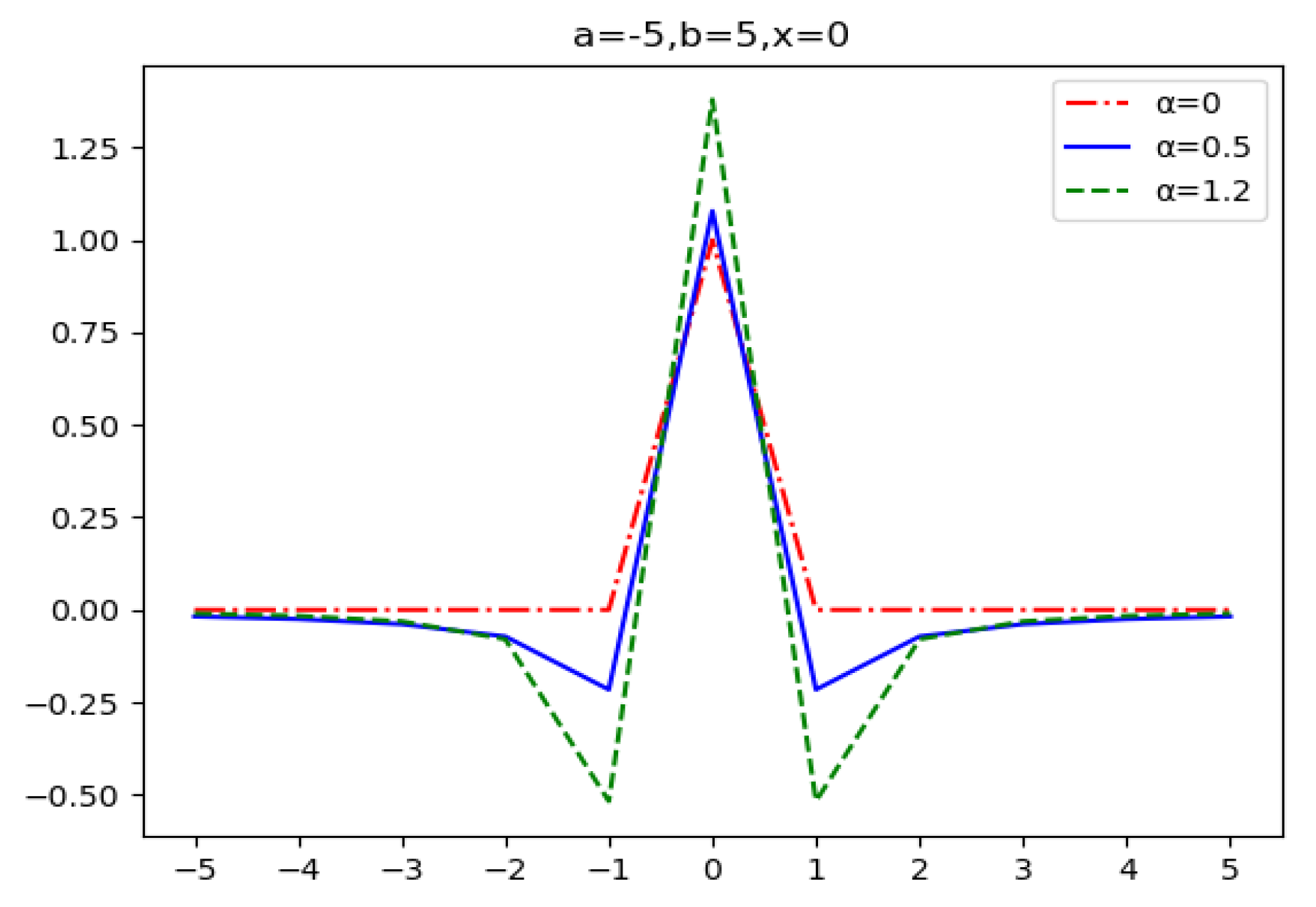
A visual representation of the vectors constructed from the coefficients of the Grünwald–Letnikov fractional derivative is shown in Figure 1, where a = 0, b = 9, and x = 5 . Figure 2 shows the vectors constructed from the coefficients of the Riesz fractional derivatives.
Comparing Figure 1 with Figure 2, we find that the shape of the two vectors is generally consistent. This means that the hypothesis of the Grünwald–Letnikov fractional derivative coefficient vectors is well founded and reasonable. However, the computational complexity of gamma functions hinders the further use of the Riesz fractional operation in deep neural networks; so, we adopt the Grünwald–Letnikov method.

3.2. From Coefficient Vectors to Category Representation Vectors

In terms of the total amount of information contained, FV contains more information than the one-hot and label smoothing. The fractional vector with n elements can represent n different characteristics, each of which can be different as the order changes. When 0 < α < 1 , the value of the non-target element is between   1   and   0 , which does not need to be positive, whereas negative probabilities exist in the physical world and are necessary in some cases [36,37,38]. In our experiments, models with FV representing categories converged more easily in some cases, perhaps providing the evidence for the existence of negative distribution.
The basic assumption for the classifier is that the greater the difference between different categories, the better. Correspondingly, the similarity of different category representation vectors must be more heterogeneous. The similarity between any two one-hot vectors is equal to 0, while the similarity between any two vectors represented by label smoothing is also equal, though not equal to 0. For a classifier with 10 classes, the cosine similarity between any two label smoothing vectors is 0.0229 if ε   is   taken   as   the   fault   value   0.1 . However, the similarity between any two adjacent FVs is negative, and the cosine similarity between any two FVs is different. The details of the data analysis can be seen in Table 1. According to the table, even without the use of AI, the average person can correctly identify the target category based on the difference in cosine similarity.
When FV is applied to DNNs, the speed of operation is intolerable. Iterative computation according to Equation (2) means to count each element repeatedly. If the number of elements counted with Pythonis greater, the computation crashes. Therefore, the iterative calculation must be changed to the sequential method. The running speed of the sequential calculation method is more than 1000 times faster than that of the iterative method. Algorithm 1 shows the few lines of codes needed to quickly construct an FV. Compared to one-hot vectors, the linear operation of FVs makes sense in the training of DNNs, as shown in the next section, where the convex combination of data [39] directly corresponds to the weighted combination of the corresponding FVs. The one-hot representation category, on the other hand, cannot be used directly for arithmetic in this way. Using the mix-up arithmetic trick described in [39], the loss function must be weighted after the individual categories have been operated on using cross-entropy loss function. Note that FVs cannot be used to calculate the loss function using cross-entropy because some of the elements of the FV are negative and cannot be logged. However, FVs can use cosine similarity to estimate the loss function for training; the effect is barely distinguishable from the cross-entropy loss function.
Algorithm 1: Codes of the sequential calculation method for the design of FVs
def lateral_index(index, alpha):
  x = []
  for i in range(index):
    if i == 0:
      tmp = 1
    else:
      tmp = (1 − (alpha + 1)/i) * tmp
    x.append(tmp)
  return x
From Figure 1 and Figure 2, we can see that FVs have the property of being non-local, which is related to the universal property of fractional calculus of being non-local and memorable. This can be used in deep neural networks and plays an important role in the generalization performance of networks, as will be shown in the next section.

4. Experiments

4.1. CIFAR-10

We conducted image classification experiments on the CIFAR-10 data sets to evaluate the generalization performance of FVs, shown in Table 2. We compared FVs with label smoothing regularization or mix-up methods [39].The data set consisted of 60,000 color images of three channels, each of which had a size of 32 × 32. There were 50,000 images in the training set and 10,000 images in the test set. We started the learning rate at 0.1 and divided it by 10 after 70 epochs or 140 epochs. ResNet18 was trained for 90 epochs, and ResNet101 was trained for 200 epochs. All the models were trained on Kaggle with a Tesla P100-GPU using pyTorch1.10. We set weight decay with 10 4 . All the methods were evaluated on the test set after training.
From Table 2, we can conclude that the generalization of FVs performed better than other methods. The small-capacity model ResNet18 with FVs plus mix-up was equivalent in performance to the high-capacity model ResNet101. For high-capacity models, FVs had no advantages, perhaps because high-capacity models already had good generalization performance. The training accuracy of the mix-up method was low because the combination of data could not directly correspond to the combination of labels in the training process. Finally, the convex combination of one-hot vectors was meaningless. However, FVs can be directly operated linearly. Therefore, the training accuracy of the FVs+mix-up method was much higher than that of the mix-up method.

4.2. CIFAR-100

We also evaluated FVs on the CIFAR-100 dataset with the result shown in Table 3. This data set contained 100 classes. Each class contained 600 32 × 32 color images, of which 500 were used as training images and 100 were used in the test set. During training, data augmentation such as random horizontal flip and color jitter were used and the learning rate was divided by 10 when the epoch was increased to 90 or 140. All the models were training on Kaggle with a Tesla P100-GPU for running 150 epochs with a mini-batch size of 128. The experiments showed that α ( 0 ,   1 ) made FVs appropriate.
For FVs, we found that FVs plus the mix-up method led to improved performance in generalization, almost more than 10 percentage points over DenseNet121 alone. We also found that there was little difference between using any regularization method alone and training DenseNet series directly.

4.3. MNIST for InfoGAN

The emergence of generative adversarial nets (GANs) [40] is an innovative milestone in deep learning; but the images generated by GANs are random and unpredictable. Conditional GANs (C-GANs) make GANs controllable with additional conditions [41]. The objective function of C-GANs can be denoted as follows [41]:
min G   max D V ( D , G ) = E x ~ P d a t a ( x ) [ log ( D ( x | y ) ] + E z ~ P z ( z ) [ log ( 1 D ( G ( z | y ) ) ) ]
where y is the condition; these can be category conditions.
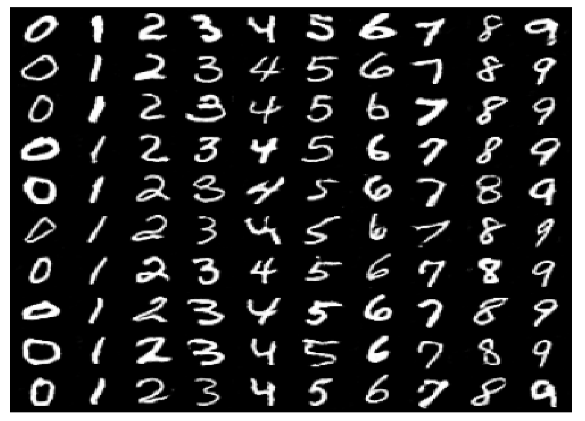
Due to the simplicity and applicability, we found that both FVs and one-hot used in C-GANs can achieve a completely correct classification effect. We could generate the images according to the categorical conditions. However, the images generated by C-GANs were blurred. Motivated by the knowledge of C-GANs, many promising methods have been proposed, such as InfoGAN [42], pix2pixGAN [43], and ACGAN [44]. FVs can provide these models with more category representation information and more degrees of freedom than one-hot or label smoothing vectors. Here, we evaluated FVs using the InfoGAN model on a MNIST data set. During the training process, we set α ( 1.0 ,   1.5 ) while the dimension of the FVs was 32 and the dimension of the noise vector was 16. The model was trained over 30 epochs. The fractional orders α that were used to generate each row of images were random numbers obeying a uniform distribution between 1 and 1.5. Experiments showed that α   in this interval produced the best quality images. From Figure 3, we can see that as the fractional order α changed, the resulting images changed consistently from line to line, such as line thickness and rotation angle, and that the image quality was better with less interference. However, adding disentangled latent codes to vectors during training to represent different meanings worked better, as explained in the paper [42].
In the previous one-hot category representation algorithm, we needed a 100-dimensional vector to represent the categories and noise samples for training the GAN model on the MNIST data set. With FVs, we only needed 48 dimensions to obtain the same or even better image quality. Similar experiments confirmed that FVs can be used for noise sampling. The results were consistent with standard normal distribution sampling.

5. Discussion and Future Directions

In this paper, we propose FVs based on the left and right Grünwald–Letnikov fractional derivatives. We showed that FVs have the performance of generalization and, as category representation vectors, FVs can be computed directly according to the combination of data. Experiments showed that FVs plus the mix-up method can produce a stronger regularization of the classification during DNNs’ training. The generic one-hot is the peculiarity of frac-vectors when the fractional order is 0. When utilized in GAN models, frac-vectors provide more information and higher degrees of freedom about the category without more computational overhead.
FVs also open up avenues for further exploration of the category representation based on the fractional calculus theory, which is still mysterious in its application to ANNs, especially in deep neural networks. There are still too many puzzles to be solved, such as how to make the non-target elements of the FVs change as training progresses and be used for image processing, just as word vectors can be trained in DNNs, and how to improve the regularization of FVs and generalization performance. Although our discussion involves the simple extension of the one-hot category representation, we are excited about the implicit layers of the fractional category representation and hope that our discussion will prove useful for further development.

Author Contributions

Conceptualization, S.T. and Y.P.; methodology, Y.P.; software, S.T. and Y.P.; validation, S.T. and Y.P.; formal analysis, S.T. and Y.P.; investigation, S.T. and Y.P.; resources, Y.P.; data curation, Y.P.; writing—original draft, S.T.; writing—review & editing, Y.P.; visualization, S.T.; supervision, Y.P.; project administration, Y.P. All authors have read and agreed to the published version of the manuscript.

Funding

Project supported in part by the National Natural Science Foundation of China (Grant No.~62171303), in part by China South Industries Group Corporation (Chengdu) Fire Control Technology Center Project (non-secret) (Grant No.~HK20-03), in part by the National Key Research and Development Program Foundation of China (Grant No.~2018YFC0830300).

Institutional Review Board Statement

Not applicable.

Informed Consent Statement

Not applicable.

Data Availability Statement

All the data were computed using our algorithm.

Acknowledgments

We, the authors, would like to thank the editor and reviewers in advance for their helpful comments.

Conflicts of Interest

The authors declare no conflict of interest.

References

  1. Oldham, K.B. The Fractional Calculus; Academic Press: Cambridge, MA, USA, 1974. [Google Scholar]
  2. Podlubny, I. Fractional Differential Equation; Academic Press: Cambridge, MA, USA, 1999. [Google Scholar]
  3. Sun, H.; Zhang, Y.; Baleanu, D.; Chen, W.; Chen, Y. A new collection of real world applications of fractional calculus in science and engineering. Commun. Nonlinear Sci. Numer. Simul. 2018, 64, 213–231. [Google Scholar] [CrossRef]
  4. Sonka, M. Image Processing, Analysis and Machine Vision; Tsinghua University Press: Beijing, China, 2011. [Google Scholar]
  5. Pu, Y.F.; Zhou, J.L.; Yuan, X. Fractional Differential Mask: A Fractional Differential-Based Approach for Multiscale Texture Enhancement. IEEE Trans. Image Process. 2010, 19, 491–511. [Google Scholar] [CrossRef] [PubMed]
  6. Yang, Q.; Chen, D.; Zhao, T.; Chen, Y. Fractional Calculus in Image Processing: A Review. Fract. Calc. Appl. Anal. 2016, 19, 1222–1249. [Google Scholar] [CrossRef] [Green Version]
  7. Zhang, X.F.; Dai, L.W. Image Enhancement Based on Rough Set and Fractional Order Differentiator. Fractal Fract. 2022, 6, 214. [Google Scholar] [CrossRef]
  8. Zhang, X.F.; Liu, R.; Ren, J.X.; Gui, Q.L. Adaptive Fractional Image Enhancement Algorithm Based on Rough Set and Particle Swarm Optimization. Fractal Fract. 2022, 6, 100. [Google Scholar] [CrossRef]
  9. Zhang, X.F.; Yan, H.; He, H. Multi-focus image fusion based on fractional-order derivative and intuitionistic fuzzy sets. Front. Inform. Technol. Elect. Eng. 2020, 21, 834–843. [Google Scholar] [CrossRef]
  10. Yan, H.; Zhang, J.X.; Zhang, X.F. Injected Infrared and Visible Image Fusion via L-1 Decomposition Model and Guided Filtering. IEEE Trans. Comput. Imaging 2022, 8, 162–173. [Google Scholar] [CrossRef]
  11. Yan, H.; Zhang, X.F. Adaptive fractional multi-scale edge-preserving decomposition and saliency detection fusion algorithm. ISA Trans. 2020, 107, 160–172. [Google Scholar] [CrossRef]
  12. Ghanbari, B.; Atangana, A. Some new edge detecting techniques based on fractional derivatives with non-local and non-singular kernels. Adv. Differ. Equ. 2020, 2020, 19. [Google Scholar] [CrossRef]
  13. Babu, N.R.; Sanjay, K.; Balasubramaniam, P. EED: Enhanced Edge Detection Algorithm via Generalized Integer and Fractional-Order Operators. Circuits Syst. Signal Process. 2022, 41, 5492–5534. [Google Scholar] [CrossRef]
  14. Jindal, N.; Singh, K. Applicability of fractional transforms in image processing—Review, technical challenges and future trends. Multimed. Tools Appl. 2019, 78, 10673–10700. [Google Scholar] [CrossRef]
  15. Yetik, I.S.; Kutay, M.A.; Ozaktas, H.; Ozaktas, H.M. Continuous and discrete fractional Fourier domain decomposition. In Proceedings of the IEEE International Conference on Acoustics, Speech, and Signal Processing, Istanbul, Turkey, 5–9 June 2000; pp. 93–96. [Google Scholar]
  16. Zhang, X.; Shen, Y.; Li, S.; Zhang, H. Medical image registration in fractional Fourier transform domain. Optik 2013, 124, 1239–1242. [Google Scholar] [CrossRef]
  17. Sharma, K.K.; Joshi, S.D. Image Registration using Fractional Fourier Transform. In Proceedings of the IEEE Asia Pacific Conference on Circuits & Systems, Singapore, 4–7 December 2006. [Google Scholar]
  18. Zhao, T.Y.; Ran, Q.W. The Weighted Fractional Fourier Transform and Its Application in Image Encryption. Math. Probl. Eng. 2019, 2019, 10. [Google Scholar] [CrossRef]
  19. Zhou, N.R.; Li, H.L.; Wang, D.; Pan, S.M.; Zhou, Z.H. Image compression and encryption scheme based on 2D compressive sensing and fractional Mellin transform. Opt. Commun. 2015, 343, 10–21. [Google Scholar] [CrossRef]
  20. Ben Farah, M.A.; Guesmi, R.; Kachouri, A.; Samet, M. A novel chaos based optical image encryption using fractional Fourier transform and DNA sequence operation. Opt. Laser Technol. 2020, 121, 8. [Google Scholar] [CrossRef]
  21. Khan, S.; Ahmad, J.; Naseem, I.; Moinuddin, M. A Novel Fractional Gradient-Based Learning Algorithm for Recurrent Neural Networks. Circuits Syst. Signal Process. 2018, 37, 593–612. [Google Scholar] [CrossRef]
  22. Wang, J.; Wen, Y.; Gou, Y.; Ye, Z.; Chen, H. Fractional-order gradient descent learning of BP neural networks with Caputo derivative. Neural Netw. 2017, 89, 19–30. [Google Scholar] [CrossRef]
  23. Yang, C.; Guangyuan, Z. A Caputo-type fractional-order gradient descent learning of deep BP neural networks. In Proceedings of the 2019 IEEE 3rd Advanced Information Management, Communicates, Electronic and Automation Control Conference (IMCEC), Chongqing, China, 11–13 October 2019. [Google Scholar] [CrossRef]
  24. Viera-Martin, E.; Gomez-Aguilar, J.F.; Solis-Perez, J.E.; Hernandez-Perez, J.A.; Escobar-Jimenez, R.F. Artificial neural networks: A practical review of applications involving fractional calculus. Eur. Phys. J. Spec. Top. 2022, 231, 2059–2095. [Google Scholar] [CrossRef]
  25. Wang, X.; Su, Y.; Luo, C.; Wang, C. A novel image encryption algorithm based on fractional order 5D cellular neural network and Fisher-Yates scrambling. PLoS ONE 2020, 15, e0236015. [Google Scholar] [CrossRef]
  26. Mani, P.; Rajan, R.; Shanmugam, L.; Joo, Y.H. Adaptive control for fractional order induced chaotic fuzzy cellular neural networks and its application to image encryption. Inf. Sci. 2019, 491, 74–89. [Google Scholar] [CrossRef]
  27. Bengio, Y.; Ducharme, R.; Vincent, P. A Neural Probabilistic Language Model. J. Mach. Learn. Res. 2003, 3, 1137–1155. [Google Scholar]
  28. Hinton, G.E. Learning and relearning in Boltzmann machines. In Parallel Distributed Processing: Explorations in the Microstructure of Cognition; MIT Press: Cambridge, MA, USA, 1986. [Google Scholar]
  29. Yoshua, B.; Goodfellow, I.; Courville, A. Deep Learning; MIT Press: Cambridge, MA, USA, 2016. [Google Scholar]
  30. Szegedy, C.; Vanhoucke, V.; Ioffe, S.; Shlens, J.; Wojna, Z. Rethinking the Inception Architecture for Computer Vision. In Proceedings of the 2016 IEEE Conference on Computer Vision and Pattern Recognition (CVPR), Seattle, WA, USA, 27–30 June 2016; pp. 2818–2826. [Google Scholar]
  31. Hinton, G.; Vinyals, O.; Dean, J. Distilling the Knowledge in a Neural Network. arXiv 2015, arXiv:1503.02531. [Google Scholar]
  32. Zhang, C.B.; Jiang, P.T.; Hou, Q.B.; Wei, Y.C.; Han, Q.; Li, Z.; Cheng, M.M. Delving Deep into Label Smoothing. IEEE Trans. Image Process. 2021, 30, 5984–5996. [Google Scholar] [CrossRef] [PubMed]
  33. Li, C.S.; Liu, C.; Duan, L.X.; Gao, P.; Zheng, K. Reconstruction Regularized Deep Metric Learning for Multi-Label Image Classification. IEEE Trans. Neural Netw. Learn. Syst. 2020, 31, 2294–2303. [Google Scholar] [CrossRef]
  34. Fa-Wang, L.; Ping-Hui, Z.; Qingxia, L. Numerical Solution of Fractional Partial Differential Equation and Its Application; Science Press: Beijing, China, 2015. [Google Scholar]
  35. Bueno-Orovio, A.; Kay, D.; Grau, V.; Rodriguez, B.; Burrage, K. Fractional diffusion models of cardiac electrical propagation: Role of structural heterogeneity in dispersion of repolarization. J. R. Soc. Interface 2014, 11, 12. [Google Scholar] [CrossRef] [Green Version]
  36. Erev, I.; Bornstein, G.; Wallsten, T.S. The Negative Effect of Probability Assessments on Decision Quality. Organ. Behav. Hum. Decis. Process. 1993, 55, 78–94. [Google Scholar] [CrossRef]
  37. Han, Y.D.; Hwang, W.Y.; Koh, I.G. Explicit solutions for negative-probability measures for all entangled states. Phys. Lett. A 1996, 221, 283–286. [Google Scholar] [CrossRef]
  38. Sokolovski, D. Weak values, “negative probability,” and the uncertainty principle. Phys. Rev. A 2007, 76, 13. [Google Scholar] [CrossRef]
  39. Zhang, H.; Cisse, M.; Dauphin, Y.N.; Lopez-Paz, D. mixup: Beyond Empirical Risk Minimization. arXiv 2017, arXiv:1710.09412. [Google Scholar]
  40. Goodfellow, I.; Pouget-Abadie, J.; Mirza, M.; Xu, B.; Warde-Farley, D.; Ozair, S.; Courville, A.; Bengio, Y. Generative Adversarial Networks. Commun. ACM 2020, 63, 139–144. [Google Scholar] [CrossRef]
  41. Mirza, M.; Osindero, S. Conditional Generative Adversarial Nets. arXiv 2014, arXiv:1411.1784. [Google Scholar]
  42. Chen, X.; Duan, Y.; Houthooft, R.; Schulman, J.; Sutskever, I.; Abbeel, P. InfoGAN: Interpretable Representation Learning by Information Maximizing Generative Adversarial Nets. arXiv 2016, arXiv:1606.03657. [Google Scholar]
  43. Isola, P.; Zhu, J.Y.; Zhou, T.H.; Efros, A.A. Image-to-Image Translation with Conditional Adversarial Networks. In Proceedings of the 30th IEEE/CVF Conference on Computer Vision and Pattern Recognition (CVPR), Honolulu, HI, USA, 21–26 July 2017; pp. 5967–5976. [Google Scholar]
  44. Odena, A.; Olah, C.; Shlens, J. Conditional Image Synthesis with Auxiliary Classifier GANs. In Proceedings of the 34th International Conference on Machine Learning, Sydney, Australia, 6–11 August 2017. [Google Scholar]
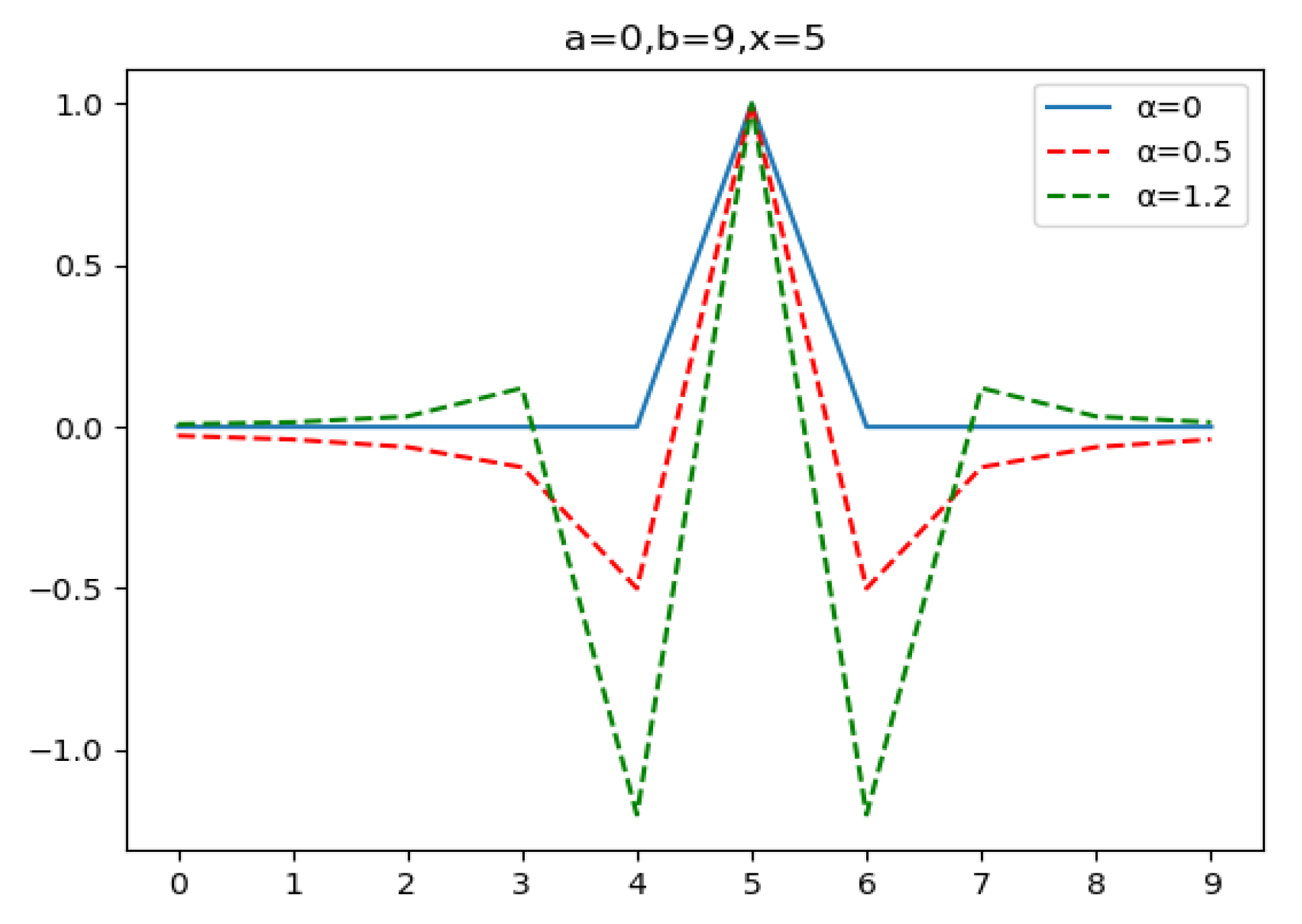
Figure 1. Coefficient vectors of left and right Grünwald–Letnikov derivatives.
Fractalfract 07 00132 g001
Figure 2. Coefficients of Riesz fractional central difference calculation method.
Fractalfract 07 00132 g002
Figure 3. Images generated from InfoGAN with FVs on the MNIST data set.
Fractalfract 07 00132 g003
Table 1. Cosine similarity between FVs, supposing there are 10 classes and α = 0.5.
0123456789
01−0.66440.02830.01820.01290.00960.00740.00570.00390.0000
1 1−0.56360.04610.02920.02050.01520.01160.00860.0039
2 1−0.55520.04880.03100.02170.01600.01160.0057
3 1−0.55300.04960.03140.02170.01520.0074
4 1−0.55250.04960.03100.02050.0096
5 1−0.55300.04880.02920.0129
6 1−0.55520.04610.0182
7 1−0.56360.0283
8 1−0.6644
9 1
Table 2. Accuracy of CIFAR-10 data set.
PlusTrain_accTest_accBest_accTop5_acc
ResNet18 1.00.14390.15000.5359
Label Smoothing1.00.40300.41000.8282
FVs0.99900.86480.90500.9451
mix-up0.75770.51940.56000.9256
FVs+mix-up0.81370.95200.95590.9888
ResNet101 0.99830.94410.95570.9986
FVs0.92360.88380.88830.9697
FVs+mix-up0.99870.94500.94500.9871
Table 3. Test accuracy on CIFAR-100 data set.
PlusTrain_accTop1_accBest_accTop5_acc
DenseNet 0.97110.57690.63280.8290
Label Smoothing0.97770.57860.61720.8255
FVs0.77770.58330.67190.7058
mix-up0.57170.55430.64420.6833
DenseNet121 0.71240.57640.63280.6847
FVs0.99300.62830.73440.7530
mix-up0.62470.58970.60140.6731
FVs+mix-up0.69120.66280.74120.8216
Disclaimer/Publisher’s Note: The statements, opinions and data contained in all publications are solely those of the individual author(s) and contributor(s) and not of MDPI and/or the editor(s). MDPI and/or the editor(s) disclaim responsibility for any injury to people or property resulting from any ideas, methods, instructions or products referred to in the content.