Abstract
In this paper, in order to improve the calculation accuracy and efficiency of α-order Caputo fractional derivative (0 < α ≤ 1), we developed a compact scheme combining the fast time stepping method for solving 2D fractional nonlinear subdiffusion equations. In the temporal direction, a time stepping method was applied. It can reach second-order accuracy. In the spatial direction, we utilized the compact difference scheme, which can reach fourth-order accuracy. Some properties of coefficients are given, which are essential for the theoretical analysis. Meanwhile, we rigorously proved the unconditional stability of the proposed scheme and gave the sharp error estimate. To overcome the intensive computation caused by the fractional operators, we combined a fast algorithm, which can reduce the computational complexity from O(N2) to O(Nlog(N)), where N represents the number of time steps. Considering that the solution of the subdiffusion equation is weakly regular in most cases, we added correction terms to ensure that the solution can achieve the optimal convergence accuracy.
1. Introduction
Fractional differential equations (FDEs) have been widely studied because of their memory effects [1,2]. Many important physical problems can finally be transformed into the solution of FDEs, such as the fractional subdiffusion equation and fractional wave equation [3,4,5]. However, in most cases, it is extremely difficult or even impossible to solve FDEs directly. This inspires us to develop numerical methods to solve FDEs. These numerical methods include the finite difference method [6,7,8], finite element method [9,10,11], finite volume method [12,13,14], Galerkin spectral method [15,16,17] and so forth. The fractional subdiffusion equations, as essential FDEs, have been widely applied in many fields, such as simulation engineering, physics and biology, and researchers have demonstrated that the use of FDEs has performed better than integer ones in the above areas [18,19,20].
In this paper, we consider the following fractional nonlinear subdiffusion equation:
where is a bounded domain, the initial value and the source term are given functions, the nonlinear term satisfies with and C is a positive constant. are Caputo fractional derivatives of order , which is defined as follows [21]:
In addition, we know that
The time stepping method plays an important role in the process of solving FDEs. Many researchers have investigated the time stepping method. Li et al. [22] utilized the time stepping method for the nonlinear fluid–fluid interaction. Zeng et al. [23] proposed a fast algorithm for the time stepping method. Alzahrani et al. [24] developed a high-order time stepping method for space fractional reaction diffusion equations. The method used in this paper in time discretization is the shifted convolution quadrature method [25], which belongs to the time stepping method. Usually, the subdiffusion equations have an initial singularity for non-smooth solutions. We improved the accuracy by adding correction terms. Due to the fact that fractional operators spend much time in computation due to their nonlocality, the fast algorithm was implemented to reduce the computational cost. Liu et al. [26] proposed a fast high-order compact difference method that can help to reduce the computational work from to in the temporal direction. We also utilized a fast algorithm that can reduce the computational work from to , where N represents the number of time steps. To the best of the authors’ knowledge, there are few papers utilizing the fast algorithm for the problem (1). The highlights of this paper can be summarized as
- Our numerical schemes have temporal second-order accuracy and spatial fourth-order accuracy, which are relatively high.
- We developed a fast time stepping method for solving the nonlinear fractional subdiffusion equation, which improves the computation efficiency.
- We recovered the optimal convergence accuracy for non-smooth solutions by adding correction terms.
This paper is organized in several sections. In Section 2, we introduce some lemmas and notations. In Section 3, the fully discrete scheme is given. In Section 4, we rigorously prove the stability of the fully discrete scheme and give the sharp error estimate. In Section 5, we derive the approximation formulas with the correction terms, which can help to improve the optimal convergence accuracy. In Section 6, we combine a fast algorithm to reduce the computational cost from to . Finally, we make a conclusion.
2. Preparations
and are evenly divided into and , respectively. Let , , , where are positive integers, are the step sizes in space along the x direction and y direction, respectively, and is the temporal step size. Define ; thus, we obtain a uniform discretization in space and time.
Define , and is covered by . , , and [0,T] is covered by .
We define the grid functions as follows:
For any , we have
Introduce the notations
Define compact operator [27]
Inner products and the responding norms are given as follows:
We have
For any , we define
and the responding norm is .
Finally, we define the grid function
Lemma 1
([28]). For any , we have
Lemma 2
([27]). For any , we have
3. Fully Discrete Compact Scheme
Lemma 3
([29]). The Caputo fractional derivative is approximated at
where , and the coefficients are as follows:
Lemma 4
([10,29]). The first-order derivative is approximated at
where \{2}.
Consider Equation (1) at nodes . We obtain
where , .
Act the operator on both sides of Equation (19). We obtain
where .
Case :
Case :
where .
Omit the error term , replace the exact solution with the numerical solution and obtain numerical schemes for solving Equation (1) as follows:
Case :
Case :
4. Stability and Convergence Analysis
Lemma 5
Lemma 6
Theorem 1.
Proof of Theorem 1.
We take the inner product of (23) and (24) with . Then, we replace l with n and sum both sides for n from 1 to N ( ). We obtain
Using the Lemmas 1, 5 and 6 and the Cauchy–Schwarz inequality, we have
Ignoring the non-negative terms, we obtain
Similarly, for , with (21) and the Cauchy–Schwarz inequality, we have
Using Grönwall’s inequality, we obtain
where C is independent of n and .
Finally, using the triangular inequality , we obtain Theorem 1. □
Theorem 2.
Assume that is the exact solution of Equation (1). Let be the numerical solution of the fully discrete scheme. We have the error estimate
where C is independent of and τ.
Proof of Theorem 2.
For simplicity, define . Note that . Using Equation (21) minus (23) and Equation (22) minus (24), we have
Case :
Case :
Both integrate , then replace n with l and sum l from 1 to n. We can obtain
We know that
For , we can similarly derive that
Using Grönwall’s inequality, we obtain
where C is independent of and . is defined by
Finally, by using the triangle inequality, we obtain Theorem 2. □
5. Analysis for Non-Smooth Solutions
By reading references [30,31], we rewrite the approximation formula with correction terms.
where the correction terms can be obtained by solving the following linear systems:
Case :
Case :
5.1. Fast Algorithm
We can obtain the following formula by referring to [29,32].
We define such that
Then, we can obtain
(60) also shows that
where .
We choose base B, and is divided into a series of small intervals as follows:
where B is an integer.
Next, we need to find the approximate formula for (61). In particular, we choose the Talbot contour as the integral pat. The Talbot contour is given as
where are parameters that we decided for ourselves. Here, we choose [29]. For the selection of parameters, readers can refer to [33] for more details.
The integral along the Talbot contour C, (61) can be approximated as
where the weights and quadrature points are given by
The choice of K has an effect on the approximation of (61). Generally, the larger the K selected, the better the approximation between different small intervals .
Since (63) overlaps the adjacent interval , points are introduced to divide the interval . satisfy
and . L is the smallest integer such that .
Now, we can rewrite the approximation Formula (16) with as follows
For convenience, we define as
Because has a recursive structure, (71) can be rewritten as
5.2. Numerical Experiments
Case 1: We consider (1) with homogeneous initial condition .
Its exact solution is , the nonlinear term is and the responding forcing term is . The corresponding results are given in Table 1 and Table 2. We also present the pictures of the numerical solution and exact solution with , in Figure 1.

Table 1.
Errors and temporal convergence orders with .
Table 2.
Errors and spatial convergence orders with and .
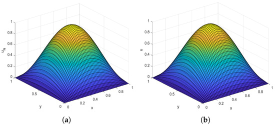
Figure 1.
Numerical solution and exact solution for Case 1 at the final time with , . (a) Numerical solution. (b) Exact solution.
Case 2: We consider (1) with non-homogeneous initial condition . Its exact solution is , the nonlinear term is and the responding forcing term is .
The responding results are shown in Table 3. We present the pictures of the numerical solution and exact solution with , in Figure 2. We can see that the numerical scheme is still applicable to the equations with initial conditions, which reflects the stability of our method.
Table 3.
Errors and temporal convergence orders with for non-homogeneous initial condition.
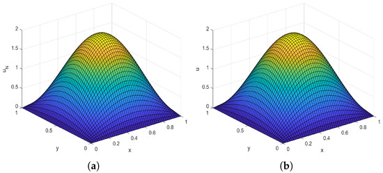
Figure 2.
Numerical solution and exact solution for Case 2 at the final time with , . (a) Numerical solution. (b) Exact solution.
Case 3: We consider the (1) with homogeneous initial condition . Its exact solution is .
Table 4 compares the results using (21), (22) and (57), (58). The standard method in Table 4 refers to the method solved directly by using the compact scheme. Because the solution has weak regularity, the convergence accuracy is not optimal and, with correction terms, it is better than the results of scheme (21) and (22).
Table 4.
Temporal convergence orders with .
Case 4: We consider the (1) with homogeneous initial condition . Its exact solution and the responding forcing term are the same as with the first case. We use for numerical solutions obtained by the standard method and for numerical solutions obtained by the fast algorithm. We calculate the pointwise error
for and , where and represent and in (73), respectively. The results are shown in Table 5. We plot the numerical solutions obtained by the standard method and the fast algorithm at , as shown in Figure 3, and the contours of pointwise error are given in Figure 4. We can clearly see that, when the time division is dense enough, the fast algorithm can reduce the calculation time and ensure the accuracy of the calculation results.
Table 5.
Pointwise error with and .
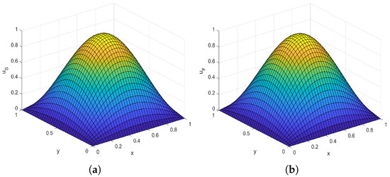
Figure 3.
Numerical solution for Case 4 at the final time with . (a) Numerical solution by standard method. (b) Numerical solution by fast algorithm.
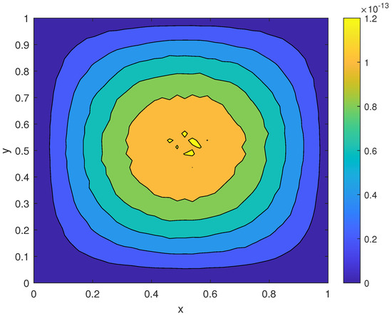
Figure 4.
Contours of pointwise error for Case 4 at the final time with .
6. Conclusions
In this study, we developed a compact scheme combining the fast time stepping method for solving fractional nonlinear subdiffusion equations. To overcome the weak regularity of nonsmooth solutions, we added the correction terms to recover the optimal convergence accuracy. We had the stability analysis for Equation (1) and gave a sharp estimate. Several numerical experiments were implemented to validate the theoretical results and confirm the efficiency and accuracy of the fast algorithm. In the future, we will use fast algorithms to solve systems composed of fractional differential equations, possibly in three dimensions. We will explore more efficient approximations for fractional operators.
Author Contributions
Methodology, Y.L.; Formal analysis, Z.W.; Data curation, L.F.; Writing—original draft, Y.X.; Writing—review & editing, X.Y. All authors have read and agreed to the published version of the manuscript.
Funding
This research was funded by National Natural Science Foundation of China grant number 11801060, 62103079.
Data Availability Statement
All data reported are obtained by the numerical schemes designed in this paper.
Conflicts of Interest
The authors declare that there is no conflict of interests regarding the publication of this paper.
References
- Chen, C.J.; Liu, H.; Zheng, X.C.; Wang, H. A two grid mmoc finite element method for nonlinear variable order time-fractional mobile immobile advection-diffusion equations. Comput. Math. Appl. 2020, 79, 2771–2783. [Google Scholar] [CrossRef]
- Liu, H.; Zheng, X.C.; Chen, C.J.; Wang, H. A characteristic finite element method for the time fractional mobile/immobile advection diffusion model. Adv. Comput. Math. 2021, 47, 1–19. [Google Scholar] [CrossRef]
- Liu, Y.Q.; Yin, X.L.; Feng, L.B.; Sun, H.G. Finite difference scheme for simulating a generalized two dimensional multi term time fractional non newtonian fluid model. Adv. Differ. Equ. 2018, 2018, 442. [Google Scholar] [CrossRef]
- Asl, M.A.; Saei, F.D.; Javidi, M.; Mahmoudi, Y. Numerical solution of fractional riesz space telegraph equation: Stability and error. Comput. Methods Differ. Equ. 2021, 9, 187–210. [Google Scholar]
- Feng, L.B.; Liu, F.W.; Turner, I.; Zheng, L.C. Novel Numerical Analysis of MultiTerm Time Fractional Viscoelastic Non Newtonian Fluid Models for Simulating Unsteady Mhd Couette Flow of a Generalized Oldroyd B Fluid. Frac. Calc. Appl. Anal. 2018, 21, 1073–1103. [Google Scholar] [CrossRef]
- Bu, W.P.; Xiao, A.G.; Zeng, W. Finite difference/finite element methods for distributed order time fractional diffusion equations. J. Sci. Comput. 2017, 72, 422–441. [Google Scholar] [CrossRef]
- Singh, J.; Gupta, P.K.; Rai, K.N. Solution of fractional bioheat equations by finite difference method and hpm. Math. Comput. Model. 2011, 54, 2316–2325. [Google Scholar] [CrossRef]
- Zhang, Y. A finite difference method for fractional partial differential equation. Appl. Math. Comput. 2009, 215, 524–529. [Google Scholar] [CrossRef]
- Zhu, X.G.; Yuan, Z.B.; Wang, J.G.; Nie, Y.F.; Yang, Z.Z. Finite element method for time space fractional schrodinger equation. Electron. J. Differ. Equ. 2017, 2017, 1–18. [Google Scholar]
- Liu, Y.; Du, Y.W.; Li, H.; Liu, F.W.; Wang, Y.J. Some second order theta schemes combined with finite element method for nonlinear fractional cable equation. Numer. Algorithms 2019, 80, 533–555. [Google Scholar] [CrossRef]
- Song, M.H.; Wang, J.F.; Liu, Y.; Li, H. Local discontinuous Galerkin method combined with the L2 formula for the time fractional Cable model. J. Appl. Math. Comput. 2022, 68, 4457–4478. [Google Scholar] [CrossRef]
- Wang, H.; Cheng, A.J.; Wang, K.X. Fast finite volume methods for space fractional diffusion equations. Discret. Contin. Dyn. Syst. Ser. B 2015, 20, 1427–1441. [Google Scholar] [CrossRef]
- Edwan, R.; Al-Omari, S.; Al-Smadi, M.; Momani, S.; Fulga, A. A new formulation of finite difference and finite volume methods for solving a space fractional convection diffusion model with fewer error estimates. Adv. Differ. Equ. 2021, 2021, 510. [Google Scholar] [CrossRef]
- Sun, Y.N.; Zhang, T. A finite difference/finite volume method for solving the fractional diffusion wave equation. J. Korean Math. Soc. 2021, 58, 553–569. [Google Scholar]
- Liu, Y.Q.; Sun, H.G.; Yin, X.L.; Feng, L.B. Fully discrete spectral method for solving a novel multi term time fractional mixed diffusion and diffusion wave equation. Z. Angew. Math. Phys. 2020, 71, 21. [Google Scholar] [CrossRef]
- Liu, Y.Q.; Yin, X.L.; Liu, F.W.; Xin, X.Y.; Shen, Y.F.; Feng, L.B. An alternating direction implicit legendre spectral method for simulating a 2D multi term time fractional oldroyd b fluid type diffusion equation. Comput. Math. Appl. 2022, 113, 160–173. [Google Scholar] [CrossRef]
- Zaky, M.A. A legendre spectral quadrature tau method for the multi term time fractional diffusion equations. Comput. Appl. Math. 2018, 37, 3525–3538. [Google Scholar] [CrossRef]
- Yin, B.L.; Liu, Y.; Li, H.; Zhang, Z.M. Efficient shifted fractional trapezoidal rule for subdiffusion problems with nonsmooth solutions on uniform meshes. Bit. Numer. Math. 2022, 62, 631–666. [Google Scholar] [CrossRef]
- Mao, W.T.; Wang, H.S.; Chen, C.J. A posteriori error estimations based on postprocessing technique for two sided fractional differential equations. Appl. Numer. Math. 2021, 167, 73–91. [Google Scholar] [CrossRef]
- Li, X.L.; Chen, Y.P.; Chen, C.J. An Improved Two grid Technique for the Nonlinear Time Fractional Parabolic Equation Based on the Block Centered Finite Difference Method. J. Comput. Math. 2022, 40, 455–473. [Google Scholar] [CrossRef]
- Podlubny, I. Fractional Differential Equations; Academic Press: Cambridge, MA, USA, 1999. [Google Scholar]
- Li, J.; Huang, P.Z.; Zhang, C.; Guo, G.H. A linear, decoupled fractional time stepping method for the nonlinear fluid fluid interaction. Numer. Methods Partial Differ. Equ. 2019, 35, 1873–1889. [Google Scholar] [CrossRef]
- Zeng, F.H.; Turner, I.; Burrage, K. A stable fast time stepping method for fractional integral and derivative operators. J. Sci. Comput. 2018, 77, 283–307. [Google Scholar] [CrossRef]
- Alzahrani, S.S.; Khaliq, A.Q.M.; Biala, T.A.; Furati, K.M. Fourth order time stepping methods with matrix transfer technique for space fractional reaction diffusion equations. Appl. Numer. Math. 2019, 146, 123–144. [Google Scholar] [CrossRef]
- Liu, Y.; Yin, B.L.; Li, H.; Zhang, Z.M. The unified theory of shifted convolution quadrature for fractional calculus. J. Sci. Comput. 2021, 89, 1–24. [Google Scholar] [CrossRef]
- Liu, Z.G.; Cheng, A.J.; Li, X.L. A fast high order compact difference method for the fractional cable equation. Numer. Methods Partial Differ. Equ. 2018, 34, 2237–2266. [Google Scholar] [CrossRef]
- Zhao, X.; Sun, Z.Z.; Hao, Z.P. A Fourth order compact ADI scheme for two dimensional nonlinear space fractional schrödinger equation. SIAM J. Sci. Comput. 2014, 36, A2865–A2886. [Google Scholar] [CrossRef]
- Sun, Z.Z. Numerical Methods for Partial Differential Equations, 2nd ed.; Science Press: Beijing, China, 2012. (In Chinese) [Google Scholar]
- Yin, B.L.; Liu, Y.; Li, H.; Zeng, F.H. A class of efficient time stepping methods for multi term time fractional reaction diffusion wave equations. Appl. Numer. Math. 2021, 165, 56–82. [Google Scholar] [CrossRef]
- Zeng, F.H.; Zhang, Z.Q.; Karniadakis, G.E. Second order numerical methods for multi term fractional differential equations: Smooth and nonsmooth solutions. Comput. Methods Appl. Mech. Eng. 2017, 327, 478–502. [Google Scholar] [CrossRef]
- Lubich, C. Discretized fractional calculus. SIAM J. Math. Anal. 1986, 17, 704–719. [Google Scholar] [CrossRef]
- Schaedle, A.; Lopez-Fernandez, M.; Lubich, C. Fast and oblivious convolution quadrature. SIAM J. Sci. Comput. 2006, 28, 421–438. [Google Scholar] [CrossRef]
- Weideman, J.A.C. Optimizing talbot’s contours for the inversion of the laplace transform. SIAM J. Numer. Anal. 2006, 44, 2342–2362. [Google Scholar] [CrossRef]
- Zeng, F.H.; Turner, I.; Burrage, K.; Karniadakis, G.E.M. A new class of semi-implicit methods with linear complexity for nonlinear fractional differential equations. SIAM J. Sci. Comput. 2018, 40, A2986–A3011. [Google Scholar] [CrossRef]


Disclaimer/Publisher’s Note: The statements, opinions and data contained in all publications are solely those of the individual author(s) and contributor(s) and not of MDPI and/or the editor(s). MDPI and/or the editor(s) disclaim responsibility for any injury to people or property resulting from any ideas, methods, instructions or products referred to in the content. |
© 2023 by the authors. Licensee MDPI, Basel, Switzerland. This article is an open access article distributed under the terms and conditions of the Creative Commons Attribution (CC BY) license (https://creativecommons.org/licenses/by/4.0/).