Mittag–Leffler Functions in Discrete Time

Abstract

In this paper, we give an efficient way to calculate the values of the Mittag–Leffler (h-ML) function defined in discrete time $h\mathbb{N}$, where $h>0$ is a real number. We construct a matrix equation that represents an iteration scheme obtained from a fractional h-difference equation with an initial condition. Fractional h-discrete operators are defined according to the Nabla operator and the Riemann–Liouville definition. Some figures and examples are given to illustrate this new calculation technique for the h-ML function in discrete time. The h-ML function with a square matrix variable in a square matrix form is also given after proving the Putzer algorithm.

1. Introduction

To emphasize the importance of studying the Mittag–Leffler (ML) function in fractional calculus, one can state that the ML function, ${\displaystyle \sum _{k=0}^{\infty }\frac{x^k}{\mathrm{\Gamma }(\gamma k+1)}}$, where $\gamma$ is a parameter, plays as important a role in fractional calculus as the exponential function ${\displaystyle \sum _{k=0}^{\infty }\frac{x^k}{\mathrm{\Gamma }(k+1)}}$ does in calculus. The study of the ML function began after Mittag–Leffler defined it in 1903 to generalize the exponential function [1]. This generalization later led us to see that this function is one of the most important functions in the study of the fractional calculus, and the work of many researchers over the years has formed a vast body of literature that explores the function in depth [2,3,4,5,6,7,8,9].

The accurate calculation of the ML function, either defined in discrete or continuous time, is challenging for mathematicians who model real-world problems. Over the years, researchers have tried to overcome this challenge by exploring some approximation techniques. For example, several of these techniques are presented in the papers [10,11,12,13,14,15,16,17,18]. Some of these approximation techniques have been adapted for commonly used computational software such as MATLAB and Mathematica. In this paper, we develop a novel approach for calculating the ML function in discrete time. Our calculation technique relies only on the values of the Euler gamma function. For this reason, our technique can be seen as an algorithm rather than an approximation approach. In addition, the discrete domain we choose allows us to verify that the discrete h-ML function approaches the continuous ML function as h approaches zero.

In the last few decades, research in fractional calculus has been applied to several fields of science [19,20,21,22,23,24,25,26,27,28,29]. Within this development, the ML function became a crucial tool in applied mathematics. Motivated by the work performed in the paper [30] by Podlubny, we focus in this paper on h-ML functions in discrete time $h\mathbb{N}$. Within $h\mathbb{N}$, we give calculation techniques for h-ML functions in several forms. The papers [31,32,33] provide some background in the field of fractional h-discrete calculus.

We organize our work in the following way: In Section 2, we provide preliminary information to aid in understanding our later work. This section includes some basic definitions in fractional h-discrete calculus along with the Riemann–Liouville definition of the fractional h-difference operator. In Section 3, we give an iteration scheme for the fractional h-discrete equation. This scheme allows us to calculate the values of the h-ML function in $h\mathbb{N}$ using approximations for the gamma function. We illustrate our results with some figures and examples. The graphs were obtained using Mathematica-13 software. In Section 4, we consider the h-ML function with an $n\times n$ matrix parameter. We develop necessary tools to prove the Putzer algorithm in order to write the h-ML function in matrix form.

2. Preliminaries

Let $h\in {\mathbb{R}}^{+}$. Denote by $h{\mathbb{N}}_m=\{m,m+h,m+2h,\cdots \}$ and $h{\mathbb{N}}_m^n=\{m,m+h,m+2h,\cdots ,n\}$ for any m, $n\in \mathbb{R}$, such that $\frac{n-m}{h}\in {\mathbb{N}}_1$.

Definition 1 

([32]). For s, $\nu \in \mathbb{R}$ and $h>0$,

$$s_h^{\overline{\nu }}=h^{\nu }\frac{\mathrm{\Gamma }(\frac{s}{h}+\nu )}{\mathrm{\Gamma }\left(\frac{s}{h}\right)},$$

where the RHS is well defined.

Definition 2 

([32]). Let $a\in \mathbb{R}$ and $\gamma \in {\mathbb{R}}^{+}$. For $x:h{\mathbb{N}}_a\to \mathbb{R}$, the γth-order sum in the nabla h-fractional sense is defined as

$${\nabla }_{h,a}^{-\gamma }x\left(t\right):=\frac{1}{\mathrm{\Gamma }\left(\gamma \right)}\sum _{r=a/h}^{t/h}{(t-\varrho \left(rh\right))}_h^{\overline{\gamma -1}}x\left(rh\right)h,t\in h{\mathbb{N}}_a,$$

where $h\in {\mathbb{R}}^{+}$ and $\varrho \left(t\right)=t-h$.

Definition 3 

([32]). For $x:h{\mathbb{N}}_a\to \mathbb{R}$, the γth-order difference in the Riemann–Liouville nabla h-fractional sense is defined as

$${\nabla }_{h,a}^{\gamma }x\left(t\right):={\nabla }_h^n{\nabla }_{h,a}^{-(n-\gamma )}x\left(t\right),t\in h{\mathbb{N}}_{a+nh},$$

where γ, $h\in {\mathbb{R}}^{+}$, $a\in \mathbb{R}$, $n-1<\gamma \le n$, and $n\in \mathbb{N}$.

Theorem 1 

([31]). Assume $x:h{\mathbb{N}}_a\to \mathbb{R}$, $\gamma \in {\mathbb{R}}^{+}$, $\gamma \notin {\mathbb{N}}_1$, and $n\in {\mathbb{N}}_1$ with $n-1<\gamma <n$. Then,

$${\nabla }_{h,a}^{\gamma }x\left(t\right)=\frac{1}{\mathrm{\Gamma }(-\gamma )}\sum _{r=a/h}^{t/h}{(t-\varrho \left(rh\right))}_h^{\overline{-\gamma -1}}x\left(rh\right)h,t\in h{\mathbb{N}}_a.$$

Lemma 1 

([32]). Let $\gamma \in {\mathbb{R}}^{+}$ and $\delta \in \mathbb{R}$, such that $\frac{\mathrm{\Gamma }(\delta +1)}{\mathrm{\Gamma }(\delta +\gamma +1)}$ and $\frac{\mathrm{\Gamma }(\delta +1)}{\mathrm{\Gamma }(\delta -\gamma +1)}$ are defined.

1. 

${\nabla }_{h,a}^{-\gamma }{(t-\varrho \left(a\right))}_h^{\overline{\delta }}=\frac{\mathrm{\Gamma }(\delta +1)}{\mathrm{\Gamma }(\delta +\gamma +1)}{(t-\varrho \left(a\right))}_h^{\overline{\delta +\gamma }}$, $t\in h{\mathbb{N}}_a$.

2. 

${\nabla }_{h,a}^{\gamma }{(t-\varrho \left(a\right))}_h^{\overline{\delta }}=\frac{\mathrm{\Gamma }(\delta +1)}{\mathrm{\Gamma }(\delta -\gamma +1)}{(t-\varrho \left(a\right))}_h^{\overline{\delta -\gamma }}$, $t\in h{\mathbb{N}}_a$.

The following composition property is valid and for the reader’s convenience, and we include its proof here.

Lemma 2. 

Let $f:h{\mathbb{N}}_a\to \mathbb{R}$ and γ, $\delta \in {\mathbb{R}}^{+}$. Then,

$${\nabla }_{h,a}^{-\gamma }{\nabla }_{h,a}^{-\delta }x\left(t\right)={\nabla }_{h,a}^{-(\gamma +\delta )}x\left(t\right)={\nabla }_{h,a}^{-\delta }{\nabla }_{h,a}^{-\gamma }x\left(t\right),t\in h{\mathbb{N}}_a.$$

Proof. 

Consider

$$\begin{array}{cc}\hfill {\nabla }_{h,a}^{-\gamma }{\nabla }_{h,a}^{-\delta }x\left(t\right)& ={\nabla }_{h,a}^{-\gamma }\left[{\nabla }_{h,a}^{-\delta }x\left(t\right)\right]\hfill \\ & ={\nabla }_{h,a}^{-\gamma }\left[\frac{h}{\mathrm{\Gamma }\left(\delta \right)}\sum _{s=a/h}^{t/h}{(t-\varrho \left(sh\right))}_h^{\overline{\delta -1}}x\left(sh\right)h\right]\hfill \\ & =\frac{h}{\mathrm{\Gamma }\left(\gamma \right)}\sum _{s=a/h}^{t/h}{(t-\varrho \left(sh\right))}_h^{\overline{\gamma -1}}\left[\frac{h}{\mathrm{\Gamma }\left(\delta \right)}\sum _{r=a/h}^{sh/h}{(sh-\varrho \left(rh\right))}_h^{\overline{\delta -1}}x\left(rh\right)h\right]h\hfill \\ & =\frac{h}{\mathrm{\Gamma }\left(\delta \right)}\sum _{r=a/h}^{t/h}x\left(rh\right)h\left[\frac{h}{\mathrm{\Gamma }\left(\gamma \right)}\sum _{s=r}^{t/h}{(t-\varrho \left(sh\right))}_h^{\overline{\gamma -1}}{(sh-\varrho \left(rh\right))}_h^{\overline{\delta -1}}h\right]\hfill \\ & =\frac{h}{\mathrm{\Gamma }\left(\delta \right)}\sum _{r=a/h}^{t/h}x\left(rh\right)h\left[{\nabla }_{h,rh}^{-\gamma }{(t-\varrho \left(rh\right))}_h^{\overline{\delta -1}}\right]\hfill \\ & =\frac{h}{\mathrm{\Gamma }\left(\delta \right)}\sum _{r=a/h}^{t/h}x\left(rh\right)h\left[\frac{\mathrm{\Gamma }\left(\delta \right)}{\mathrm{\Gamma }(\gamma +\delta )}{(t-\varrho \left(rh\right))}_h^{\overline{\gamma +\delta -1}}\right]\hfill \\ & =\frac{h}{\mathrm{\Gamma }(\gamma +\delta )}\sum _{r=a/h}^{t/h}{(t-\varrho \left(rh\right))}_h^{\overline{\gamma +\delta -1}}x\left(rh\right)h\hfill \\ & ={\nabla }_{h,a}^{-(\gamma +\delta )}x\left(t\right),\hfill \end{array}$$

where we used item 1 in Lemma 1. The proof is complete. □

3. $\mathit{h}$-Discrete Mittag–Leffler Function

Definition 4. 

Let λ, μ, $a\in \mathbb{R}$ and h, $\upsilon \in {\mathbb{R}}^{+}$. The discrete h-ML function with two parameters is defined by

$$e_{\lambda ,\upsilon ,\mu }^h(t,a)=\left(1-\lambda h^{\upsilon }\right)\frac{1}{h^{\mu }}\sum _{k=0}^{\infty }{\lambda }^k\frac{{(t-\varrho \left(a\right))}_h^{\overline{\upsilon k+\mu }}}{\mathrm{\Gamma }(\upsilon k+\mu +1)},t\in h{\mathbb{N}}_a.$$

Clearly, $e_{\lambda ,\upsilon ,\mu }^h(a,a)=1$.

Remark 1. 

It follows from [20] that $e_{\lambda ,\upsilon ,\upsilon -1}^h(t,a)$ converges absolutely if $|\lambda h^{\upsilon }|<1$. As it was stated in [31], for each $t\in h{\mathbb{N}}_0$, the following approximation can be proven

$$\underset{h\to 0}{lim}\left[\frac{h^{\upsilon -1}}{\left(1-\lambda h^{\upsilon }\right)}{e}_{\lambda ,\upsilon ,\upsilon -1}^h(t,0)\right]=t^{\upsilon -1}{e}_{\upsilon ,\upsilon }\left(\lambda t^{\upsilon }\right),$$

where ${\displaystyle e_{\gamma ,\delta }\left(t\right)=\sum _{k=0}^{\infty }\frac{t^k}{\mathrm{\Gamma }(\gamma k+\delta )},\gamma >0,\delta >0.}$ With this note, we want to correct the misprint in the approximation statement in [31].

Next, we list some properties of the h-ML function. Henceforth, we will call this function the h-discrete Mittag–Leffler function.

Proposition 1. 

The following are valid.

1. 

For $\gamma >0$, ${\nabla }_{h,a}^{-\gamma }{e}_{\lambda ,\upsilon ,\mu }^h(t,a)=h^{\gamma }{e}_{\lambda ,\upsilon ,\mu +\gamma }^h(t,a)$, $t\in h{\mathbb{N}}_a$.

2. 

For $\gamma >0$, ${\nabla }_{h,a}^{\gamma }{e}_{\lambda ,\upsilon ,\mu }^h(t,a)=h^{-\gamma }{e}_{\lambda ,\upsilon ,\mu -\gamma }^h(t,a)$, $t\in h{\mathbb{N}}_a$.

3. 

For $\gamma \in {\mathbb{R}}^{+}\backslash {\mathbb{N}}_1$ and $n\in {\mathbb{N}}_1$, $e_{\lambda ,\gamma ,-n}^h(t,a)=\lambda h^{\gamma }{e}_{\lambda ,\gamma ,\gamma -n}^h(t,a)$, $t\in h{\mathbb{N}}_{a+h}$.

4. 

For $n\in {\mathbb{N}}_1$ and $\gamma \in (0,n)\backslash {\mathbb{N}}_1$, ${\nabla }_{h,a}^{\gamma }{e}_{\lambda ,\gamma ,\gamma -n}^h(t,a)=\lambda e_{\lambda ,\gamma ,\gamma -n}^h(t,a)$, $t\in h{\mathbb{N}}_{a+h}$.

5. 

For $\gamma \ge 1$ and $0<\lambda h^{\gamma }<1$, $e_{\lambda ,\gamma ,\gamma -1}^h(t,a)$ is monotone increasing on $h{\mathbb{N}}_a$.

Proof. 

For $t\in h{\mathbb{N}}_a$, consider

$$\begin{array}{cc}\hfill & {\nabla }_{h,a}^{-\gamma }{e}_{\lambda ,\upsilon ,\mu }^h(t,a)\hfill \\ \hfill & =\frac{h}{\mathrm{\Gamma }\left(\gamma \right)}\sum _{s=a/h}^{t/h}{(t-\varrho \left(sh\right))}_h^{\overline{\gamma -1}}{e}_{\lambda ,\upsilon ,\mu }^h(sh,a)\hfill \\ \hfill & =\frac{h}{\mathrm{\Gamma }\left(\gamma \right)}\sum _{s=a/h}^{t/h}{(t-\varrho \left(sh\right))}_h^{\overline{\gamma -1}}\left[\left(1-\lambda h^{\upsilon }\right)\frac{1}{h^{\mu }}\sum _{k=0}^{\infty }{\lambda }^k\frac{{(sh-\varrho \left(a\right))}_h^{\overline{\upsilon k+\mu }}}{\mathrm{\Gamma }(\upsilon k+\mu +1)}\right]\hfill \\ & =\left(1-\lambda h^{\upsilon }\right)\frac{1}{h^{\mu }}\sum _{k=0}^{\infty }\frac{{\lambda }^k}{\mathrm{\Gamma }(\upsilon k+\mu +1)}\left[\frac{h}{\mathrm{\Gamma }\left(\gamma \right)}\sum _{s=a/h}^{t/h}{(t-\varrho \left(sh\right))}_h^{\overline{\gamma -1}}{(sh-\varrho \left(a\right))}_h^{\overline{\upsilon k+\mu }}\right]\hfill \\ & =\left(1-\lambda h^{\upsilon }\right)\frac{1}{h^{\mu }}\sum _{k=0}^{\infty }\frac{{\lambda }^k}{\mathrm{\Gamma }(\upsilon k+\mu +1)}\left[{\nabla }_{h,a}^{-\gamma }{(t-\varrho \left(a\right))}_h^{\overline{\upsilon k+\mu }}\right]\hfill \\ & =\left(1-\lambda h^{\upsilon }\right)\frac{1}{h^{\mu }}\sum _{k=0}^{\infty }\frac{{\lambda }^k}{\mathrm{\Gamma }(\upsilon k+\mu +1)}\left[\frac{\mathrm{\Gamma }(\upsilon k+\mu +1)}{\mathrm{\Gamma }(\upsilon k+\mu +\gamma +1)}{(t-\varrho \left(a\right))}_h^{\overline{\upsilon k+\mu +\gamma }}\right]\hfill \\ & =\left(1-\lambda h^{\upsilon }\right)\frac{1}{h^{\mu }}\sum _{k=0}^{\infty }{\lambda }^k\frac{{(t-\varrho \left(a\right))}_h^{\overline{\upsilon k+\mu +\gamma }}}{\mathrm{\Gamma }(\upsilon k+\mu +\gamma +1)}\hfill \\ & =h^{\gamma }{e}_{\lambda ,\upsilon ,\mu +\gamma }^h(t,a),\hfill \end{array}$$

where we used item 1. in Lemma 1. This completes the proof of item 1. Since the proof of item 2 is similar to the proof of item 1, we omit it. Next, we continue with the proof of item 3. For $\gamma \in {\mathbb{R}}^{+}\backslash {\mathbb{N}}_1$, $n\in {\mathbb{N}}_1$ and $t\in h{\mathbb{N}}_{a+h}$, we have

$$\begin{array}{cc}\hfill e_{\lambda ,\gamma ,-n}^h(t,a)& =\left(1-\lambda h^{\gamma }\right)\frac{1}{h^{-n}}\sum _{k=0}^{\infty }{\lambda }^k\frac{{(t-\varrho \left(a\right))}_h^{\overline{\gamma k-n}}}{\mathrm{\Gamma }(\gamma k-n+1)}\hfill \\ & =\left(1-\lambda h^{\gamma }\right)\frac{1}{h^{-n}}\frac{{(t-\varrho \left(a\right))}_h^{\overline{-n}}}{\mathrm{\Gamma }(-n+1)}+\left(1-\lambda h^{\gamma }\right)\frac{1}{h^{-n}}\sum _{k=1}^{\infty }{\lambda }^k\frac{{(t-\varrho \left(a\right))}_h^{\overline{\gamma k-n}}}{\mathrm{\Gamma }(\gamma k-n+1)}\hfill \\ & =0+\left(1-\lambda h^{\gamma }\right)\frac{1}{h^{-n}}\sum _{k=0}^{\infty }{\lambda }^{k+1}\frac{{(t-\varrho \left(a\right))}_h^{\overline{\gamma k+\gamma -n}}}{\mathrm{\Gamma }(\gamma k+\gamma -n+1)}\hfill \\ & =\lambda \left(1-\lambda h^{\gamma }\right)\frac{1}{h^{-n}}\sum _{k=0}^{\infty }{\lambda }^k\frac{{(t-\varrho \left(a\right))}_h^{\overline{\gamma k+\gamma -n}}}{\mathrm{\Gamma }(\gamma k+\gamma -n+1)}\hfill \\ & =\lambda h^{\gamma }{e}_{\lambda ,\gamma ,\gamma -n}^h(t,a).\hfill \end{array}$$

This completes the proof of item 3. For the proof of item 4, consider $t\in h{\mathbb{N}}_{a+h}$. Using items 2 and 3, we have

$$\begin{array}{cc}\hfill {\nabla }_{h,a}^{\gamma }{e}_{\lambda ,\gamma ,\gamma -n}^h(t,a)& =h^{-\gamma }{e}_{\lambda ,\gamma ,-n}^h(t,a)\hfill \\ \hfill & =\lambda e_{\lambda ,\gamma ,\gamma -n}^h(t,a).\hfill \end{array}$$

Hence, the proof of item 4 is complete. The proof of item 5 relies on the fact that if ${\nabla }_{h}x\left(t\right)\ge 0$ on $h{\mathbb{N}}_{a+h}$, then f is increasing on $h{\mathbb{N}}_a$. For $t\in h{\mathbb{N}}_{a+h}$, consider

$$\begin{array}{cc}\hfill {\nabla }_h{e}_{\lambda ,\gamma ,\gamma -1}^h(t,a)& =e_{\lambda ,\gamma ,\gamma -2}^h(t,a)(\mathrm{using}\left(2\right))\hfill \\ & =\left(1-\lambda h^{\gamma }\right)\frac{1}{h^{\gamma -2}}\sum _{k=0}^{\infty }{\lambda }^k\frac{{(t-\varrho \left(a\right))}_h^{\overline{\gamma k+\gamma -2}}}{\mathrm{\Gamma }(\gamma k+\gamma -1)}\hfill \\ & =\left(1-\lambda h^{\gamma }\right)\sum _{k=0}^{\infty }\frac{{\left(\lambda h^{\gamma }\right)}^k}{\mathrm{\Gamma }(\gamma k+\gamma -1)}\frac{\mathrm{\Gamma }(\frac{t-a}{h}+\gamma k+\gamma -1)}{\mathrm{\Gamma }\left(\frac{t-a}{h}\right)}.\hfill \end{array}$$

For $h>0$, $\gamma \ge 1$, $0<\lambda h^{\gamma }<1$, $t\in h{\mathbb{N}}_{a+h}$ and $k\in {\mathbb{N}}_0$, $\mathrm{\Gamma }(\frac{t-a}{h}+\gamma k+\gamma -1)>0$, $\mathrm{\Gamma }\left(\frac{t-a}{h}\right)>0$, $\mathrm{\Gamma }(\gamma k+\gamma -1)>0$ and ${\left(\lambda h^{\gamma }\right)}^k>0$, implying that

$${\nabla }_h{e}_{\lambda ,\gamma ,\gamma -1}^h(t,a)>0,t\in h{\mathbb{N}}_{a+h}.$$

Thus, $e_{\lambda ,\gamma ,\gamma -1}^h(t,a)$ is monotone increasing on $h{\mathbb{N}}_a$. The proof of item 5 is complete. □

Theorem 2. 

Assume $\lambda \in \mathbb{R}$, $h\in {\mathbb{R}}^{+}$, $n\in {\mathbb{N}}_{}$, $\gamma \in (n-1,n)$, such that $|\lambda h^{\gamma }|<1$. The linear homogeneous h-difference equation

$${\nabla }_{h,a}^{\gamma }y\left(t\right)=\lambda y\left(t\right),t\in h{\mathbb{N}}_{a+nh},$$

(1)

has a general solution

$$y\left(t\right)=C_1{e}_{\lambda ,\gamma ,\gamma -1}^h(t,a)+C_2{e}_{\lambda ,\gamma ,\gamma -2}^h(t,a)+\cdots C_n{e}_{\lambda ,\gamma ,\gamma -n}^h(t,a),t\in h{\mathbb{N}}_a,$$

(2)

where $C_1$, $C_2,\cdots ,C_n$ are constants.

Proof. 

Fix $1\le i\le n$. From Proposition 1 (4), we have

$${\nabla }_{h,a}^{\gamma }{e}_{\lambda ,\gamma ,\gamma -i}^h(t,a)=\lambda e_{\lambda ,\gamma ,\gamma -i}^h(t,a),$$

for $t\in h{\mathbb{N}}_{a+h}$. Hence, for each $1\le i\le n$, $e_{\lambda ,\gamma ,\gamma -i}^h(t,a)$ is a solution of (1) on $h{\mathbb{N}}_a$. It follows that a general solution of (1) is given by (2). The proof is complete. □

Corollary 1. 

Assume $\lambda \in \mathbb{R}$, $h\in {\mathbb{R}}^{+}$, $0<\gamma <1$, such that $|\lambda h^{\gamma }|<1$. The IVP

$$\left\{\begin{array}{c}{\nabla }_{h,0}^{\gamma }y\left(t\right)=\lambda y\left(t\right),t\in h{\mathbb{N}}_h,\hfill \\ y\left(0\right)=1,\hfill \end{array}\right.$$

(3)

has the unique solution

$$y\left(t\right)=e_{\lambda ,\gamma ,\gamma -1}^h(t,0),t\in h{\mathbb{N}}_0.$$

(4)

3.1. A Way to Compute $e_{\lambda ,\gamma ,\gamma -1}^h(t,0)$

Let $m\in {\mathbb{N}}_1$ and consider the IVP associated with (3):

$$\left\{\begin{array}{c}{\nabla }_{h,0}^{\gamma }w\left(t\right)=\lambda w\left(t\right),t\in h{\mathbb{N}}_h^{mh},\hfill \\ w\left(0\right)=1,\hfill \end{array}\right.$$

(5)

Rewriting the equation in (5) using Theorem 1, we have

$$\frac{1}{\mathrm{\Gamma }(-\gamma )}\sum _{s=0}^{t/h}{(t-\varrho \left(sh\right))}_h^{\overline{-\gamma -1}}w\left(sh\right)h=\lambda w\left(t\right),t\in h{\mathbb{N}}_h^{mh}.$$

(6)

Denote by

$${\mathcal{H}}_{-\gamma -1}^h(t,\varrho \left(sh\right))=\frac{{(t-\varrho \left(sh\right))}_h^{\overline{-\gamma -1}}}{\mathrm{\Gamma }(-\gamma )},s\in {\mathbb{N}}_0^{t/h},t\in h{\mathbb{N}}_h^{mh}.$$

Rearranging the terms in (6), we obtain

$$\left(h^{-\gamma }-\lambda \right)w\left(t\right)+\sum _{s=1}^{t/h-1}{\mathcal{H}}_{-\gamma -1}^h(t,\varrho \left(sh\right))w\left(sh\right)h=-{\mathcal{H}}_{-\gamma -1}^h(t,\varrho \left(0\right))w\left(0\right)h,t\in h{\mathbb{N}}_h^{mh},$$

(7)

that is

$$w\left(t\right)+\frac{h^{\gamma +1}}{1-\lambda h^{\gamma }}\sum _{s=1}^{t/h-1}{\mathcal{H}}_{-\gamma -1}^h(t,\varrho \left(sh\right))w\left(sh\right)=-\frac{h^{\gamma +1}}{1-\lambda h^{\gamma }}{\mathcal{H}}_{-\gamma -1}^h(t,\varrho \left(0\right)),t\in h{\mathbb{N}}_h^{mh},$$

(8)

Denote by $\mathrm{\Omega }=\frac{h^{\gamma +1}}{1-\lambda h^{\gamma }}$ and $\tilde{w}={[w\left(h\right),w\left(2h\right),\cdots ,w\left(mh\right)]}^T$. Then, the matrix form of (8) is given by

$$\mathcal{L}\tilde{w}=-\mathcal{B},$$

where

$$\mathcal{L}=\left(\begin{array}{cccccc}1& 0& \cdots & \cdots & 0& 0\\ \mathrm{\Omega }{\mathcal{H}}_{-\gamma -1}^h(2h,\varrho \left(h\right))& 1& \cdots & \cdots & 0& 0\\ \mathrm{\Omega }{\mathcal{H}}_{-\gamma -1}^h(3h,\varrho \left(h\right))& \mathrm{\Omega }{\mathcal{H}}_{-\gamma -1}^h(3h,\varrho \left(2h\right))& \cdots & \cdots & 0& 0\\ ⋮& ⋮& ⋮& ⋮& ⋮& ⋮\\ ⋮& ⋮& ⋮& ⋮& ⋮& ⋮\\ \mathrm{\Omega }{\mathcal{H}}_{-\gamma -1}^h(mh-h,\varrho \left(h\right))& \mathrm{\Omega }{\mathcal{H}}_{-\gamma -1}^h(mh-h,\varrho \left(2h\right))& \cdots & \cdots & 1& 0\\ \mathrm{\Omega }{\mathcal{H}}_{-\gamma -1}^h(mh,\varrho \left(h\right))& \mathrm{\Omega }{\mathcal{H}}_{-\gamma -1}^h(mh,\varrho \left(2h\right))& \cdots & \cdots & \mathrm{\Omega }{\mathcal{H}}_{-\gamma -1}^h(mh,\varrho (mh-h))& 1\end{array}\right)$$

is a lower triangular-strip matrix and

$$\mathcal{B}=\mathrm{\Omega }\left(\begin{array}{c}{\mathcal{H}}_{-\gamma -1}^h(h,\varrho \left(0\right))\\ {\mathcal{H}}_{-\gamma -1}^h(2h,\varrho \left(0\right))\\ {\mathcal{H}}_{-\gamma -1}^h(3h,\varrho \left(0\right))\\ ⋮\\ ⋮\\ {\mathcal{H}}_{-\gamma -1}^h(mh-h,\varrho \left(0\right))\\ {\mathcal{H}}_{-\gamma -1}^h(mh,\varrho \left(0\right))\end{array}\right).$$

Since $\mathcal{L}$ is non-singular, it follows from (4) that

$$\left(\begin{array}{c}{e}_{\lambda ,\gamma ,\gamma -1}^h(h,0)\\ e_{\lambda ,\gamma ,\gamma -1}^h(2h,0)\\ e_{\lambda ,\gamma ,\gamma -1}^h(3h,0)\\ ⋮\\ ⋮\\ e_{\lambda ,\gamma ,\gamma -1}^h(mh-h,0)\\ e_{\lambda ,\gamma ,\gamma -1}^h(mh,0)\end{array}\right)=-{\mathcal{L}}^{-1}\mathcal{B}.$$

Here, $\mathcal{L}={\left[{\mathcal{L}}_{ij}\right]}_{m\times m}$ and $\mathcal{B}={\left[{\mathcal{B}}_i\right]}_{m\times 1}$, where

$${\mathcal{L}}_{ij}=\left\{\begin{array}{c}1,i=j,\hfill \\ 0,i<j,\hfill \\ \mathrm{\Omega }{\mathcal{H}}_{-\gamma -1}^h(ih,\varrho \left(jh\right)),i>j,\hfill \end{array}\right.$$

and

$${\mathcal{B}}_i=\mathrm{\Omega }{\mathcal{H}}_{-\gamma -1}^h(ih,\varrho \left(0\right)).$$

Next, we illustrate the method of calculating the discrete h-ML function with two examples. We first consider $\lambda$ as a negative real number and then $\lambda$ as a positive real number. In both examples, our results for $h=1$ coincide with the calculation of the discrete h-ML function $e^1$ in the paper [34].

Example 1. 

Computation of $e_{-0.5,\gamma ,\gamma -1}^h(t,0)$ for $t\in h{\mathbb{N}}_h^{10h}$.

If $\gamma =0.5$ and $h=1$, then we have

$$\mathcal{L}=\left(\begin{array}{cccccccccc}1.0000& 0& 0& 0& 0& 0& 0& 0& 0& 0\\ -0.3333& 1.0000& 0& 0& 0& 0& 0& 0& 0& 0\\ -0.0833& -0.3333& 1.0000& 0& 0& 0& 0& 0& 0& 0\\ -0.0417& -0.0833& -0.3333& 1.0000& 0& 0& 0& 0& 0& 0\\ -0.0260& -0.0417& -0.0833& -0.3333& 1.0000& 0& 0& 0& 0& 0\\ -0.0182& -0.0260& -0.0417& -0.0833& -0.3333& 1.0000& 0& 0& 0& 0\\ -0.0137& -0.0182& -0.0260& -0.0417& -0.0833& -0.3333& 1.0000& 0& 0& 0\\ -0.0107& -0.0137& -0.0182& -0.0260& -0.0417& -0.0833& -0.3333& 1.0000& 0& 0\\ -0.0087& -0.0107& -0.0137& -0.0182& -0.0260& -0.0417& -0.0833& -0.3333& 1.0000& 0\\ -0.0073& -0.0087& -0.0107& -0.0137& -0.0182& -0.0260& -0.0417& -0.0833& -0.3333& 1.0000\end{array}\right),$$

$$\mathcal{B}=\left(\begin{array}{c}-0.3333\\ -0.0833\\ -0.0417\\ -0.0260\\ -0.0182\\ -0.0137\\ -0.0107\\ -0.0087\\ -0.0073\\ -0.0062\end{array}\right).$$

Then, we have

$$\left(\begin{array}{c}{e}_{-0.5,0.5,-0.5}^h(h,0)\\ e_{-0.5,0.5,-0.5}^h(2h,0)\\ e_{-0.5,0.5,-0.5}^h(3h,0)\\ ⋮\\ ⋮\\ e_{-0.5,0.5,-0.5}^h(9h,0)\\ e_{-0.5,0.5,-0.5}^h(10h,0)\end{array}\right)=-{\mathcal{L}}^{-1}\mathcal{B}=\left(\begin{array}{c}0.3333\\ 0.1944\\ 0.1343\\ 0.1009\\ 0.0798\\ 0.0654\\ 0.0550\\ 0.0472\\ 0.0411\\ 0.0362\end{array}\right).$$

After using the matrix method to calculate the h-ML function values, we then seek to visualize the impact of parameter changes on the graphs generated (see Figure 1). Plotting over $t\in h{\mathbb{N}}_h^{10h}$ for $\lambda =-0.5$, $h=1$, and $\gamma \in [0.1,0.9]$, we obtain the result in Figure 1a. Note that the function is only defined at integer values between 1 and 10, even though we connect the points for ease of visualization.

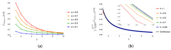
Figure 1. Family of graphs of the h-ML functions when $\lambda =-0.5$. (a) $e_{-0.5,\gamma ,\gamma -1}^1(t,0)$. (b) $e_{-0.5,0.5,-0.5}^h(t,0)$.

More interestingly, plotting over $t\in h{\mathbb{N}}_h^{10h}$ for $\lambda =-0.5$, $\gamma =0.5$, and $h\in (0,1]$, we obtain the result in Figure 1b. In addition, the continuous plot graphs $t^{-0.5}{e}_{0.5,0.5}(-0.5t^{0.5})$ are evaluated over $t\in [1,10]$. From this, we can discern that

$${\displaystyle \frac{h^{-0.5}}{1-0.5h^{0.5}}{e}_{-0.5,0.5,-0.5}^h(t,0)\to t^{-0.5}{e}_{0.5,0.5}(-0.5t^{0.5})} as h\to 0,$$

which is consistent with Remark 1. It is apparent that the discrete case approaches the continuous case as $h\to 0$.

Example 2. 

Computation of $e_{0.5,\gamma ,\gamma -1}^h(t,0)$ for $t\in h{\mathbb{N}}_h^{10h}$.

Once again, after using the matrix method to calculate the h-ML function values, we then seek to visualize the impact of parameter changes on the graphs generated. Plotting over $t\in h{\mathbb{N}}_h^{10h}$ for $\lambda =0.5$, $h=1$, and $\gamma \in [0.1,0.9]$, we obtain the result in Figure 2a. Note that the function is only defined at integer values between 1 and 10, even though we connect the points for ease of visualization.

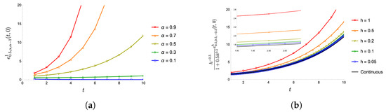
Figure 2. Family of graphs of the h-ML functions when $\lambda =0.5$. (a) $e_{0.5,\gamma ,\gamma -1}^1(t,0)$. (b) $e_{0.5,0.5,-0.5}^h(t,0)$.

It is interesting to note that plotting over $t\in h{\mathbb{N}}_h^{10h}$ for $\lambda =0.5$, $\gamma =0.5$, and $h\in (0,1]$, we obtain the result in Figure 2b. In addition, the continuous plot graphs $t^{-0.5}{e}_{0.5,0.5}\left(0.5t^{0.5}\right)$ are evaluated over $t\in [1,10]$. The figure confirms the validity of the approximation in Remark 1

${\displaystyle \frac{h^{-0.5}}{1+0.5h^{0.5}}{e}_{0.5,0.5,-0.5}^h(t,0)\to t^{-0.5}{e}_{0.5,0.5}\left(0.5t^{0.5}\right)}$ as $h\to 0$.

3.2. An Initial Value Problem

Let $m\in {\mathbb{N}}_1$ and consider the IVP

$$\left\{\begin{array}{c}{\nabla }_{h,0}^{\gamma }w\left(t\right)=a\left(t\right)w\left(t\right)+x\left(t\right),t\in h{\mathbb{N}}_h^{mh},\hfill \\ w\left(0\right)=c,\hfill \end{array}\right.$$

(9)

where a is $f:{\mathbb{N}}_h^{mh}\to \mathbb{R}$, such that

$$a\left(t\right)\ne h^{-\gamma },t\in {\mathbb{N}}_h^{mh}.$$

Denote by $\tilde{w}={[w\left(h\right),w\left(2h\right),\cdots ,w\left(mh\right)]}^T$ and $\mathcal{F}={[x\left(h\right),x\left(2h\right),\cdots ,x\left(mh\right)]}^T$.Then, the matrix form of (9) is given by

$$\mathcal{M}\tilde{w}=\mathcal{F}-\mathcal{C},$$

where

$$\mathcal{M}=\left(\begin{array}{cccccc}{h}^{-\gamma }-a\left(h\right)& 0& \cdots & \cdots & 0& 0\\ h{\mathcal{H}}_{-\gamma -1}^h(2h,\varrho \left(h\right))& h^{-\gamma }-a\left(2h\right)& \cdots & \cdots & 0& 0\\ h{\mathcal{H}}_{-\gamma -1}^h(3h,\varrho \left(h\right))& h{\mathcal{H}}_{-\gamma -1}^h(3h,\varrho \left(2h\right))& \cdots & \cdots & 0& 0\\ ⋮& ⋮& ⋮& ⋮& ⋮& ⋮\\ ⋮& ⋮& ⋮& ⋮& ⋮& ⋮\\ h{\mathcal{H}}_{-\gamma -1}^h(mh-h,\varrho \left(h\right))& h{\mathcal{H}}_{-\gamma -1}^h(mh-h,\varrho \left(2h\right))& \cdots & \cdots & h^{-\gamma }-a(mh-h)& 0\\ h{\mathcal{H}}_{-\gamma -1}^h(mh,\varrho \left(h\right))& h{\mathcal{H}}_{-\gamma -1}^h(mh,\varrho \left(2h\right))& \cdots & \cdots & h{\mathcal{H}}_{-\gamma -1}^h(mh,\varrho (mh-h))& h^{-\gamma }-a\left(mh\right)\end{array}\right)$$

is a lower triangular-strip matrix and

$$\mathcal{C}=ch\left(\begin{array}{c}{\mathcal{H}}_{-\gamma -1}^h(h,\varrho \left(0\right))\\ {\mathcal{H}}_{-\gamma -1}^h(2h,\varrho \left(0\right))\\ {\mathcal{H}}_{-\gamma -1}^h(3h,\varrho \left(0\right))\\ ⋮\\ ⋮\\ {\mathcal{H}}_{-\gamma -1}^h(mh-h,\varrho \left(0\right))\\ {\mathcal{H}}_{-\gamma -1}^h(mh,\varrho \left(0\right))\end{array}\right).$$

Since $\mathcal{M}$ is non-singular, the solution of (9) can be computed by the following numerical algorithm:

$$\left(\begin{array}{c}w\left(h\right)\\ w\left(2h\right)\\ w\left(3h\right)\\ ⋮\\ ⋮\\ w(mh-h)\\ w\left(mh\right)\end{array}\right)={\mathcal{M}}^{-1}[\mathcal{F}-\mathcal{C}].$$

Here, $\mathcal{M}={\left[{\mathcal{M}}_{ij}\right]}_{m\times m}$ and $\mathcal{C}={\left[{\mathcal{C}}_i\right]}_{m\times 1}$, where

$${\mathcal{M}}_{ij}=\left\{\begin{array}{c}{h}^{-\gamma }-a\left(ih\right),i=j,\hfill \\ 0,i<j,\hfill \\ h{\mathcal{H}}_{-\gamma -1}^h(ih,\varrho \left(jh\right)),i>j,\hfill \end{array}\right.$$

and

$${\mathcal{C}}_i=ch{\mathcal{H}}_{-\gamma -1}^h(ih,\varrho \left(0\right)).$$

Now, we are in a position to state and prove the general solution to the linear nonhomogeneous nabla fractional h-difference equation.

Theorem 3. 

Let $\lambda \in \mathbb{R}$, $h\in {\mathbb{R}}^{+}$, $n\in \mathbb{N}$, $\gamma \in (n-1,n)$, such that $|\lambda h^{\gamma }|<1$ and $g:h{\mathbb{N}}_a\to \mathbb{R}$. The general solution of the linear nonhomogeneous nabla fractional h-difference equation

$${\nabla }_{h,a}^{\gamma }y\left(t\right)=\lambda y\left(t\right)+\mathcal{G}\left(t\right),t\in h{\mathbb{N}}_{a+nh},$$

(10)

is given by

$$\begin{array}{c}y\left(t\right)=C_1{e}_{\lambda ,\gamma ,\gamma -1}^h(t,a)+C_2{e}_{\lambda ,\gamma ,\gamma -2}^h(t,a)+\cdots C_n{e}_{\lambda ,\gamma ,\gamma -n}^h(t,a)\hfill \\ \hfill +\frac{1}{\left(1-\lambda h^{\gamma }\right)}\sum _{s=a/h+1}^{t/h}{e}_{\lambda ,\gamma ,\gamma -1}^h(t,sh)\mathcal{G}\left(sh\right)h^{\gamma },t\in h{\mathbb{N}}_a,\end{array}$$

(11)

where $C_1$, $C_2,\cdots ,C_n$ are constants.

Proof. 

In view of Theorem 2, it suffices to show that

$$\frac{1}{\left(1-\lambda h^{\gamma }\right)}\sum _{s=a/h+1}^{t/h}{e}_{\lambda ,\gamma ,\gamma -1}^h(t,sh)\mathcal{G}\left(sh\right)h^{\gamma }$$

is a particular solution of (10). Denote by

$$x\left(t\right)=\frac{1}{\left(1-\lambda h^{\gamma }\right)}\sum _{s=a/h+1}^{t/h}{e}_{\lambda ,\gamma ,\gamma -1}^h(t,sh)\mathcal{G}\left(sh\right)h^{\gamma },t\in h{\mathbb{N}}_a.$$

It is enough to show that

$${\nabla }_{h,a}^{\gamma }x\left(t\right)=\lambda x\left(t\right)+\mathcal{G}\left(t\right),t\in h{\mathbb{N}}_{a+nh}.$$

(12)

To see this, for $t\in h{\mathbb{N}}_a$, consider

$$\begin{array}{cc}\hfill x\left(t\right)& =\frac{1}{\left(1-\lambda h^{\gamma }\right)}\sum _{s=a/h+1}^{t/h}{e}_{\lambda ,\gamma ,\gamma -1}^h(t,sh)\mathcal{G}\left(sh\right)h^{\gamma }\hfill \\ \hfill & =\frac{1}{\left(1-\lambda h^{\gamma }\right)}\sum _{s=a/h+1}^{t/h}\left[\left(1-\lambda h^{\gamma }\right)\frac{1}{h^{\gamma -1}}\sum _{k=0}^{\infty }{\lambda }^k\frac{{(t-\varrho \left(sh\right))}_h^{\overline{\gamma k+\gamma -1}}}{\mathrm{\Gamma }(\gamma k+\gamma )}\right]\mathcal{G}\left(sh\right)h^{\gamma }\hfill \\ \hfill & =\sum _{k=0}^{\infty }{\lambda }^k\left[\sum _{s=a/h+1}^{t/h}\frac{{(t-\varrho \left(sh\right))}_h^{\overline{\gamma k+\gamma -1}}}{\mathrm{\Gamma }(\gamma k+\gamma )}\mathcal{G}\left(sh\right)h\right]\hfill \\ \hfill & =\sum _{k=0}^{\infty }{\lambda }^k\left[\sum _{s=a/h}^{t/h}\frac{{(t-\varrho \left(sh\right))}_h^{\overline{\gamma k+\gamma -1}}}{\mathrm{\Gamma }(\gamma k+\gamma )}\mathcal{G}\left(sh\right)h-\frac{{(t-\varrho \left(a\right))}_h^{\overline{\gamma k+\gamma -1}}}{\mathrm{\Gamma }(\gamma k+\gamma )}\mathcal{G}\left(a\right)h\right]\hfill \\ & =\sum _{k=0}^{\infty }{\lambda }^k\left[{\nabla }_{h,a}^{-(\gamma k+\gamma )}\mathcal{G}\left(t\right)\right]-\mathcal{G}\left(a\right)\frac{h^{\gamma }}{\left(1-\lambda h^{\gamma }\right)}{e}_{\lambda ,\gamma ,\gamma -1}^h(t,a).\hfill \end{array}$$

(13)

Now, consider

$$\begin{array}{cc}\hfill {\nabla }_{h,a}^{\gamma }x\left(t\right)& ={\nabla }_{h,a}^{\gamma }\left[\sum _{k=0}^{\infty }{\lambda }^k\left[{\nabla }_{h,a}^{-(\gamma k+\gamma )}\mathcal{G}\left(t\right)\right]\right]-\mathcal{G}\left(a\right)\frac{h^{\gamma }}{\left(1-\lambda h^{\gamma }\right)}{\nabla }_{h,a}^{\gamma }{e}_{\lambda ,\gamma ,\gamma -1}^h(t,a)\hfill \\ & ={\nabla }_h^n{\nabla }_{h,a}^{-(n-\gamma )}\left[\sum _{k=0}^{\infty }{\lambda }^k\left[{\nabla }_{h,a+h}^{-(\gamma k+\gamma )}\mathcal{G}\left(t\right)\right]\right]-\lambda \mathcal{G}\left(a\right)\frac{h^{\gamma }}{\left(1-\lambda h^{\gamma }\right)}{e}_{\lambda ,\gamma ,\gamma -1}^h(t,a)\hfill \\ & =\sum _{k=0}^{\infty }{\lambda }^k{\nabla }_h^n\left[{\nabla }_{h,a}^{-(n-\gamma )}{\nabla }_{h,a}^{-(\gamma k+\gamma )}\mathcal{G}\left(t\right)\right]-\lambda \mathcal{G}\left(a\right)\frac{h^{\gamma }}{\left(1-\lambda h^{\gamma }\right)}{e}_{\lambda ,\gamma ,\gamma -1}^h(t,a)\hfill \\ & =\sum _{k=0}^{\infty }{\lambda }^k\left[{\nabla }_h^n{\nabla }_{h,a}^{-(\gamma k+n)}\mathcal{G}\left(t\right)\right]-\lambda \mathcal{G}\left(a\right)\frac{h^{\gamma }}{\left(1-\lambda h^{\gamma }\right)}{e}_{\lambda ,\gamma ,\gamma -1}^h(t,a)\hfill \\ & =\sum _{k=0}^{\infty }{\lambda }^k{\nabla }_{h,a}^{-\gamma k}\mathcal{G}\left(t\right)-\lambda \mathcal{G}\left(a\right)\frac{h^{\gamma }}{\left(1-\lambda h^{\gamma }\right)}{e}_{\lambda ,\gamma ,\gamma -1}^h(t,a)\hfill \\ & =\mathcal{G}\left(t\right)+\sum _{k=1}^{\infty }{\lambda }^k{\nabla }_{h,a}^{-\gamma k}\mathcal{G}\left(t\right)-\lambda \mathcal{G}\left(a\right)\frac{h^{\gamma }}{\left(1-\lambda h^{\gamma }\right)}{e}_{\lambda ,\gamma ,\gamma -1}^h(t,a)\hfill \\ & =\mathcal{G}\left(t\right)+\lambda \left[\sum _{k=0}^{\infty }{\lambda }^k{\nabla }_{h,a}^{-(\gamma k+\gamma )}\mathcal{G}\left(t\right)-\mathcal{G}\left(a\right)\frac{h^{\gamma }}{\left(1-\lambda h^{\gamma }\right)}{e}_{\lambda ,\gamma ,\gamma -1}^h(t,a)\right]\hfill \\ & =\lambda x\left(t\right)+\mathcal{G}\left(t\right),\hfill \end{array}$$

where we used Lemma 2. The proof is complete. □

4. Matrix $\mathit{h}$-Discrete Mittag–Leffler Function

In this section, we replace the scalar $\lambda$ by an $n\times n$ matrix A in the h-ML function. Our goal is to write the matrix h-ML function in discrete time as an $n\times n$ matrix function.

Definition 5. 

Consider the vector spaces ${\mathbb{R}}^n$ of all ordered n-tuples of real numbers and $M_n$ of all $n\times n$ matrices over $\mathbb{R}$. Corresponding to each vector norm on ${\mathbb{R}}^n$, we define an operator norm on $M_n$ by

$$\parallel A\parallel =\underset{\parallel y\parallel =1}{max}\parallel Ay\parallel ,$$

for any $y\in {\mathbb{R}}^n$ and $A\in M_n$. We observe that $\parallel I_n\parallel =1$, where $I_n$ denotes the $n\times n$ identity matrix.

Theorem 4 

([35]). Let R be the radius of convergence of a scalar power series

$$\sum _{k=0}^{\infty }{a}_k{x}^k$$

and let $A\in M_n$ be given with $\parallel A\parallel <R$. Then, the matrix power series

$$\sum _{k=0}^{\infty }{a}_k{A}^k$$

converges if $\overline{\varrho }\left(A\right)<R$. Here, $\overline{\varrho }\left(A\right)$ denotes the spectral radius of the matrix A.

Remark 2. 

Let λ, μ, $a\in \mathbb{R}$ and h, $\upsilon \in {\mathbb{R}}^{+}$. Fix $t\in h{\mathbb{N}}_a$. We know that the radius of convergence of the scalar power series

$$\sum _{k=0}^{\infty }{\lambda }^k\frac{{(t-\varrho \left(a\right))}_h^{\overline{\upsilon k+\mu }}}{\mathrm{\Gamma }(\upsilon k+\mu +1)}$$

is $h^{-\upsilon }$. Let $A\in M_n$, such that $\parallel A\parallel <h^{-\upsilon }$. Then, by Theorem 4, the matrix power series

$$\frac{{(t-\varrho \left(a\right))}_h^{\overline{\upsilon k+\mu }}}{\mathrm{\Gamma }(\upsilon k+\mu +1)}$$

converges if $\overline{\varrho }\left(A\right)<h^{-\upsilon }$. Define

$$e_{A,\upsilon ,\mu }^h(t,a)=\left(I_n-h^{\upsilon }A\right)\frac{1}{h^{\mu }}\sum _{k=0}^{\infty }{A}^k\frac{{(t-\varrho \left(a\right))}_h^{\overline{\upsilon k+\mu }}}{\mathrm{\Gamma }(\upsilon k+\mu +1)},t\in h{\mathbb{N}}_a.$$

(14)

Proposition 2. 

Let $0<\gamma <1$. The following are valid.

1. 

$e_{A,\gamma ,\gamma -1}^h(a,a)=I_n$.

2. 

${\nabla }_{h,a}^{\gamma }{e}_{A,\gamma ,\gamma -1}^h(t,a)=A{e}_{A,\gamma ,\gamma -1}^h(t,a)$, $t\in h{\mathbb{N}}_{a+h}$.

Theorem 5. 

Let $A\in M_n$, $h\in {\mathbb{R}}^{+}$ and $0<\gamma <1$, such that $\overline{\varrho }\left(A\right)<h^{-\gamma }$ and $g:h{\mathbb{N}}_a\to {\mathbb{R}}^n$. The IVP

$$\left\{\begin{array}{c}{\nabla }_{h,a}^{\gamma }y\left(t\right)=Ay\left(t\right)+\mathcal{G}\left(t\right),t\in h{\mathbb{N}}_{a+nh},\hfill \\ {\nabla }_{h,a}^{-(1-\gamma )}y\left(t\right){|}_{t=a}=y\left(a\right)=y_0,\hfill \end{array}\right.$$

(15)

has the unique solution

$$y\left(t\right)=e_{A,\gamma ,\gamma -1}^h(t,a)y_0+\frac{1}{\left(I_n-h^{\gamma }A\right)}\sum _{s=a/h+1}^{t/h}{e}_{A,\gamma ,\gamma -1}^h(t,sh)\mathcal{G}\left(sh\right)h^{\gamma },t\in h{\mathbb{N}}_a.$$

(16)

The Putzer algorithm is a tool to write $e^A$ in an $n\times n$ matrix form for a given $n\times n$ matrix $A.$ Here, we adopt the idea of this algorithm to write the matrix h-ML function $e_{A,\gamma ,\gamma -1}^h(t,a)$ in an $n\times n$ matrix form. This algorithm allows us to express $e_{A,\gamma ,\gamma -1}^h(t,a)$ in terms of $e_{\lambda ,\gamma ,\gamma -1}^h(t,a)$, where $\lambda$ is an eigenvalue of the matrix A.

Definition 6 

(Matrix Exponential Function). Let $A\in M_n$, $h\in {\mathbb{R}}^{+}$ and $0<\gamma <1$, such that $\overline{\varrho }\left(A\right)<h^{-\gamma }$. The IVP

$$\left\{\begin{array}{c}{\nabla }_{h,a}^{\gamma }Y\left(t\right)=AY\left(t\right),t\in h{\mathbb{N}}_{a+h},\hfill \\ {\nabla }_{h,a}^{-(1-\gamma )}Y\left(t\right){|}_{t=a}=Y\left(a\right)=I_n,\hfill \end{array}\right.$$

(17)

has the unique solution, which is called the matrix exponential function. Here, $I_n$ is the $n\times n$ identity matrix.

Theorem 6. 

Let $A\in M_n$, $h\in {\mathbb{R}}^{+}$ and $0<\gamma <1$, such that $\overline{\varrho }\left(A\right)<h^{-\gamma }$. If ${\lambda }_1,{\lambda }_2,\cdots ,{\lambda }_n$ are (not necessarily distinct) eigenvalues of the $n\times n$ matrix A, with each eigenvalue repeated as many times as its multiplicity, then

$$e_{A,\gamma ,\gamma -1}^h(t,a)=\sum _{i=0}^{n-1}{p}_{i+1}\left(t\right)M_i,$$

(18)

where

$$\begin{array}{c}{M}_0=I_n,\end{array}$$

(19)

$$\begin{array}{c}{M}_i=(A-{\lambda }_i{I}_n)M_{i-1},1\le i\le n-1,\end{array}$$

(20)

$$\begin{array}{c}{M}_n=0,\end{array}$$

(21)

and the vector’s valued function p defined by

$$\left(\begin{array}{c}{p}_1\left(t\right)\\ p_2\left(t\right)\\ p_3\left(t\right)\\ \cdots \\ p_n\left(t\right)\end{array}\right)$$

(22)

is the solution of the IVP

$$\left\{\begin{array}{c}{\nabla }_{h,a}^{\gamma }p\left(t\right)=\left(\begin{array}{ccccc}{\lambda }_1& 0& 0& 0& 0\\ 1& {\lambda }_2& 0& 0& 0\\ 0& 1& {\lambda }_3& \cdots & 0\\ ⋮& \ddots & \ddots & \ddots & ⋮\\ 0& 0& \cdots & 1& {\lambda }_n\end{array}\right)p\left(t\right),t\in h{\mathbb{N}}_{a+h},\hfill \\ {\nabla }_{h,a}^{-(1-\gamma )}p\left(t\right){|}_{t=a}=p\left(a\right)=\left(\begin{array}{c}1\\ 0\\ 0\\ \cdots \\ 0\end{array}\right).\hfill \end{array}\right.$$

(23)

Proof. 

Let

$$\mathsf{\Phi }\left(t\right)=\sum _{i=0}^{n-1}{p}_{i+1}\left(t\right)M_i.$$

We first show that $\mathsf{\Phi }$ solves the IVP (17). First, note that

$${\nabla }_{h,a}^{-(1-\gamma )}\mathsf{\Phi }\left(a\right)={\nabla }_{h,a}^{-(1-\gamma )}{p}_1\left(a\right)M_0+{\nabla }_{h,a}^{-(1-\gamma )}{p}_2\left(a\right)M_1+\cdots {\nabla }_{h,a}^{-(1-\gamma )}{p}_n\left(a\right)M_{n-1}=I_n.$$

Now, consider

$$\begin{array}{cc}\hfill & {\nabla }_{h,a}^{\gamma }\mathsf{\Phi }\left(t\right)-A\mathsf{\Phi }\left(t\right)\hfill \\ & ={\nabla }_{h,a}^{\gamma }\left[\sum _{i=0}^{n-1}{p}_{i+1}\left(t\right)M_i\right]-A\sum _{i=0}^{n-1}{p}_{i+1}\left(t\right)M_i\hfill \\ & =\sum _{i=0}^{n-1}{\nabla }_{h,a}^{\gamma }{p}_{i+1}\left(t\right)M_i-A\sum _{i=0}^{n-1}{p}_{i+1}\left(t\right)M_i\hfill \\ & ={\nabla }_{h,a}^{\gamma }{p}_1\left(t\right)M_0+\sum _{i=1}^{n-1}{\nabla }_{h,a}^{\gamma }{p}_{i+1}\left(t\right)M_i-A\sum _{i=0}^{n-1}{p}_{i+1}\left(t\right)M_i\hfill \\ & ={\lambda }_1{p}_1\left(t\right)M_0+\sum _{i=1}^{n-1}\left[p_i\left(t\right)+{\lambda }_{i+1}{p}_{i+1}\left(t\right)\right]M_i-A\sum _{i=0}^{n-1}{p}_{i+1}\left(t\right)M_i\hfill \\ & =\sum _{i=1}^{n-1}{p}_i\left(t\right)M_i+\sum _{i=0}^{n-1}{\lambda }_{i+1}{p}_{i+1}\left(t\right)M_i-A\sum _{i=0}^{n-1}{p}_{i+1}\left(t\right)M_i\hfill \\ & =\sum _{i=1}^{n-1}{p}_i\left(t\right)M_i+\sum _{i=0}^{n-1}{p}_{i+1}\left(t\right)({\lambda }_{i+1}{I}_n-A)M_i\hfill \\ & =\sum _{i=1}^{n-1}{p}_i\left(t\right)(A-{\lambda }_i{I}_n)M_{i-1}+\sum _{i=1}^n{p}_i\left(t\right)({\lambda }_i{I}_n-A)M_{i-1}\hfill \\ & =p_n\left(t\right)({\lambda }_n{I}_n-A)M_{n-1}\hfill \\ & =-p_n\left(t\right)(A-{\lambda }_n{I}_n)\prod _{j=1}^{n-1}(A-{\lambda }_j{I}_n)M_0\hfill \\ & =0.\hfill \end{array}$$

Since $e_{A,\gamma ,\gamma -1}^h(t,a)$ satisfies the IVP (17), we have

$$\mathsf{\Phi }\left(t\right)=e_{A,\gamma ,\gamma -1}^h(t,a),$$

by the unique solution of given IVP. The proof is complete. □

Example 3. 

Let $h\in {\mathbb{R}}^{+}$ and $0<\gamma <1$, such that $0.75<h^{-\gamma }$. Consider the IVP

$$\left\{\begin{array}{c}{\nabla }_{h,a}^{\gamma }Y\left(t\right)=\left(\begin{array}{ccc}\frac{1}{4}& 0& 0\\ 1& \frac{1}{2}& 1\\ 0& 0& \frac{3}{4}\end{array}\right)Y\left(t\right),t\in h{\mathbb{N}}_{a+h},0<\gamma <1,\hfill \\ {\nabla }_{h,a}^{-(1-\gamma )}Y\left(t\right){|}_{t=a}=Y\left(a\right)=I_3.\hfill \end{array}\right.$$

(24)

The eigenvalues of $A=\left(\begin{array}{ccc}\frac{1}{4}& 0& 0\\ 1& \frac{1}{2}& 1\\ 0& 0& \frac{3}{4}\end{array}\right)$ are ${\lambda }_1=\frac{1}{4}$, ${\lambda }_2=\frac{1}{2}$ and ${\lambda }_3=\frac{3}{4}$. Clearly, $\overline{\varrho }\left(A\right)=0.75<h^{-\gamma }$. We have

$$\begin{array}{cc}\hfill M_0& =I_3=\left(\begin{array}{ccc}1& 0& 0\\ 0& 1& 0\\ 0& 0& 1\end{array}\right),\hfill \\ \hfill M_1& =(A-{\lambda }_1{I}_3)M_0=\left(\begin{array}{ccc}0& 0& 0\\ 1& \frac{1}{4}& 1\\ 0& 0& \frac{1}{2}\end{array}\right),\hfill \\ \hfill M_2& =(A-{\lambda }_2{I}_3)M_1=\left(\begin{array}{ccc}-\frac{1}{4}& 0& 0\\ 1& 0& 1\\ 0& 0& \frac{1}{4}\end{array}\right)\left(\begin{array}{ccc}0& 0& 0\\ 1& \frac{1}{4}& 1\\ 0& 0& \frac{1}{2}\end{array}\right)=\left(\begin{array}{ccc}0& 0& 0\\ 0& 0& \frac{1}{2}\\ 0& 0& \frac{1}{8}\end{array}\right),\hfill \\ \hfill M_3& =0\hfill \end{array}$$

and the vector’s valued function p defined by

$$\left(\begin{array}{c}{p}_1\left(t\right)\\ p_2\left(t\right)\\ p_3\left(t\right)\end{array}\right)$$

(25)

is the solution of the IVP

$$\left\{\begin{array}{c}{\nabla }_{h,a}^{\gamma }p\left(t\right)=\left(\begin{array}{ccc}\frac{1}{4}& 0& 0\\ 1& \frac{1}{2}& 0\\ 0& 1& \frac{3}{4}\end{array}\right)p\left(t\right),t\in h{\mathbb{N}}_{a+h},\hfill \\ {\nabla }_{h,a}^{-(1-\gamma )}p\left(t\right){|}_{t=a}=p\left(a\right)=\left(\begin{array}{c}1\\ 0\\ 0\end{array}\right).\hfill \end{array}\right.$$

(26)

The equivalent form of (26) is given by

$$\left\{\begin{array}{c}{\nabla }_{h,a}^{\gamma }{p}_1\left(t\right)=\frac{1}{4}{p}_1\left(t\right),t\in h{\mathbb{N}}_{a+h},\hfill \\ {\nabla }_{h,a}^{-(1-\gamma )}{p}_1\left(t\right){|}_{t=a}=p_1\left(a\right)=1,\hfill \end{array}\right.$$

(27)

$$\left\{\begin{array}{c}{\nabla }_{h,a}^{\gamma }{p}_2\left(t\right)=p_1\left(t\right)+\frac{1}{2}{p}_2\left(t\right),t\in h{\mathbb{N}}_{a+h},\hfill \\ {\nabla }_{h,a}^{-(1-\gamma )}{p}_2\left(t\right){|}_{t=a}=p_2\left(a\right)=0,\hfill \end{array}\right.$$

(28)

$$\left\{\begin{array}{c}{\nabla }_{h,a}^{\gamma }{p}_3\left(t\right)=p_2\left(t\right)+\frac{3}{4}{p}_3\left(t\right),t\in h{\mathbb{N}}_{a+h},\hfill \\ {\nabla }_{h,a}^{-(1-\gamma )}{p}_3\left(t\right){|}_{t=a}=p_3\left(a\right)=0.\hfill \end{array}\right.$$

(29)

Using Theorem 2, the unique solution of the IVP (27) is given by

$$p_1\left(t\right)=e_{\frac{1}{4},\gamma ,\gamma -1}^h(t,a),t\in h{\mathbb{N}}_a.$$

(30)

Using Theorem 3, the unique solution of the IVP (28) is given by

$$p_2\left(t\right)=\frac{1}{\left(1-\frac{h^{\gamma }}{2}\right)}\sum _{s=a/h+1}^{t/h}{e}_{\frac{1}{2},\gamma ,\gamma -1}^h(t,sh)p_1\left(sh\right)h^{\gamma },t\in h{\mathbb{N}}_a.$$

(31)

Using Theorem 3, the unique solution of the IVP (29) is given by

$$p_3\left(t\right)=\frac{1}{\left(1-\frac{3h^{\gamma }}{4}\right)}\sum _{s=a/h+1}^{t/h}{e}_{\frac{3}{4},\gamma ,\gamma -1}^h(t,sh)p_2\left(sh\right)h^{\gamma },t\in h{\mathbb{N}}_a.$$

(32)

Thus, the matrix h-ML function is in the following a $3\times 3$ matrix form

$$\begin{array}{cc}\hfill e_{A,\gamma ,\gamma -1}^h(t,a)& =p_1\left(t\right)M_0+p_2\left(t\right)M_1+p_3\left(t\right)M_2\hfill \\ & =p_1\left(t\right)\left(\begin{array}{ccc}1& 0& 0\\ 0& 1& 0\\ 0& 0& 1\end{array}\right)+p_2\left(t\right)\left(\begin{array}{ccc}0& 0& 0\\ 1& \frac{1}{4}& 1\\ 0& 0& \frac{1}{2}\end{array}\right)+p_3\left(t\right)\left(\begin{array}{ccc}0& 0& 0\\ 0& 0& \frac{1}{2}\\ 0& 0& \frac{1}{8}\end{array}\right)\hfill \\ & =\left(\begin{array}{ccc}{p}_1\left(t\right)& 0& 0\\ p_2\left(t\right)& p_1\left(t\right)+\frac{p_2\left(t\right)}{4}& p_2\left(t\right)+\frac{p_3\left(t\right)}{2}\\ 0& 0& p_1\left(t\right)+\frac{p_2\left(t\right)}{2}+\frac{p_3\left(t\right)}{8}\end{array}\right).\hfill \end{array}$$

Developing the stability, controllability, and observability of systems of fractional h-difference equations is one important application for the use of the main results of this section.

5. Conclusions

In this paper, we demonstrated the validity of the following approximation with some examples.

$${\displaystyle \underset{h\to 0}{lim}\left[{\displaystyle \sum _{k=0}^{\infty }{\lambda }^k\frac{{(t+h)}_h^{\overline{\upsilon k+\upsilon -1}}}{\mathrm{\Gamma }(\upsilon k+\upsilon )}}\right]=t^{\upsilon -1}\sum _{k=0}^{\infty }\frac{{\left(\lambda t^{\upsilon }\right)}^k}{\mathrm{\Gamma }(\upsilon k+\upsilon )},}$$

where $0<\upsilon <1$. We made this possible by developing a novel matrix method to calculate the h-ML function on the domain $h\mathbb{N}$. This calculation technique may be considered an algorithm rather than an approximation, and such a characteristic makes this calculation method unique and reliable. In addition, we proved the Putzer algorithm in fractional h-discrete calculus, which allowed us to express the matrix h-ML function in $n\times n$ matrix form.

References

- Mittag–Leffler, G.M. Sur la nouvelle fonction eγ(x). C. R. Acad. Sci. Paris 1903, 137, 554–558. [Google Scholar]
- Adel, A.A.; Tamer, M.S.; Abdelhamid, A. Third-order differential subordination for meromorphic functions associated with generalized Mittag–Leffler function. Fractal Fract. 2023, 7, 175. [Google Scholar]
- Gorenflo, R.; Kilbas, A.A.; Mainardi, F. Mittag–Leffler Functions, Related Topics and Applications; Springer: Berlin/Heidelberg, Germany, 2014. [Google Scholar]
- Gorenflo, R.; Mainardi, F.; Rogosin, S. Mittag–Leffler function: Properties and applications. Handb. Fract. Calc. Appl. 2019, 1, 269–296. [Google Scholar]
- Haubold, H.J.; Mathai, A.M.; Saxena, R.K. Mittag–Leffler functions and their applications. J. Appl. Math. 2011, 2011, 298628. [Google Scholar] [CrossRef]
- Nagai, A. Discrete Mittag–Leffler function and its applications. Publ. Res. Inst. Math. Sci. Kyoto Univ. 2003, 1302, 1–20. [Google Scholar]
- Rogosin, S. The role of the Mittag–Leffler function in fractional modeling. Mathematics 2015, 3, 368–381. [Google Scholar] [CrossRef]
- Saenko, V.V. The calculation of the Mittag–Leffler function. Int. J. Comput. Math. 2022, 99, 1367–1394. [Google Scholar] [CrossRef]
- Saima, R.; Zakia, H.; Rehana, A.; Yu-Ming, C. New computation of unified bounds via a more general fractional operator using generalized Mittag–Leffler function in the kernel. Comput. Model. Eng. Sci. 2021, 126, 359–378. [Google Scholar]
- Garrappa, R. Numerical evaluation of two and three parameter Mittag–Leffler functions. SIAM J. Numer. Anal. 2015, 53, 1350–1369. [Google Scholar] [CrossRef]
- Garrappa, R.; Popolizio, M. Computing the matrix Mittag–Leffler function with applications to fractional calculus. J. Sci. Comput. 2018, 77, 129–153. [Google Scholar] [CrossRef]
- Hilfer, R.; Seybold, H.J. Computation of the generalized Mittag–Leffler function and its inverse in the complex plane. Integral Transform. Spec. Funct. 2006, 17, 637–652. [Google Scholar] [CrossRef]
- Li, A.; Wei, Y.; Li, Z.; Wang, Y. The numerical algorithms for discrete Mittag–Leffler functions approximation. Fract. Calc. Appl. Anal. 2019, 22, 95–112. [Google Scholar] [CrossRef]
- Naz, S.; Yu-Ming, C. A unified approach for novel estimates of inequalities via discrete fractional calculus techniques. Alex. Eng. J. 2022, 61, 847–854. [Google Scholar] [CrossRef]
- Popolizio, M. On the matrix Mittag–Leffler function: Theoretical properties and numerical computation. Mathematics 2019, 7, 1140. [Google Scholar] [CrossRef]
- Saima, R.; Yu-Ming, C.; Singh, J.; Kumar, D. A unifying computational framework for novel estimates involving discrete fractional calculus approaches. Alex. Eng. J. 2021, 60, 2677–2685. [Google Scholar]
- Seybold, H.; Hilfer, R. Numerical algorithm for calculating the generalized Mittag–Leffler function. SIAM J. Numer. Anal. 2008, 47, 69–88. [Google Scholar] [CrossRef]
- Wu, G.C.; Baleanu, D.; Zeng, S.D.; Luo, W.H. Mittag–Leffler function for discrete fractional modelling. J. King Saud Univ. Sci. 2016, 28, 99–102. [Google Scholar] [CrossRef]
- Atangana, A. Application of fractional calculus to epidemiology. In Fractional Dynamics; De Gruyter Open Poland: Warsaw, Poland, 2015; pp. 174–190. [Google Scholar]
- Atıcı, F.M.; Nguyen, N.; Dadashova, K.; Pedersen, S.E.; Koch, G. Pharmacokinetics and pharmacodynamics models of tumor growth and anticancer effects in discrete time. Comput. Math. Biophys. 2020, 8, 114–125. [Google Scholar] [CrossRef]
- Khan, A.; Bai, X.; Ilyas, M.; Rauf, A.; Xie, W.; Yan, P.; Zhang, B. Design and application of an interval estimator for nonlinear discrete-time SEIR epidemic models. Fractal Fract. 2022, 6, 213. [Google Scholar] [CrossRef]
- Kumar, S.; Pandey, R.K.; Kumar, K.; Kamal, S.; Dinh, T.N. Finite difference- collocation method for the generalized fractional diffusion equation. Fractal Fract. 2022, 6, 387. [Google Scholar] [CrossRef]
- Magin, R. Fractional Calculus in Bioengineering; Begell House Publishers Inc.: Danbury, CT, USA, 2004. [Google Scholar]
- Makhlouf, A.B.; Baleanu, D. Finite time stability of fractional order systems of neutral type. Fractal Fract. 2022, 6, 289. [Google Scholar] [CrossRef]
- Muresan, C.I.; Ostalczyk, P.; Ortigueira, M.D. Fractional calculus applications in modeling and design of control systems. J. Appl. Nonlinear Dyn. 2017, 6, 131–134. [Google Scholar] [CrossRef]
- Ostalczyk, P. Discrete Fractional Calculus: Applications in Control and Image Processing; World Scientific: Singapore, 2015. [Google Scholar]
- Podlubny, I. Fractional Differential Equations; Academic Press: New York, NY, USA, 1999. [Google Scholar]
- Samko, G.; Kilbas, A.A.; Marichev, O.I. Fractional Integrals and Derivatives: Theory and Applications; Gordon and Breach: Yverdon, Switzerland, 1993. [Google Scholar]
- Sopasakis, P.; Sarimveis, H.; Macheras, P.; Dokoumetzidis, A. Fractional calculus in pharmacokinetics. J. Pharmacokinet Pharmacodyn. 2018, 45, 107–125. [Google Scholar] [CrossRef]
- Podlubny, I. Matrix approach to discrete fractional calculus. Fract. Calc. Appl. Anal. 2000, 3, 359–386. [Google Scholar]
- Atıcı, F.M.; Chang, S.; Jonnalagadda, J. Grünwald-Letnikov fractional operators: From past to present. Fract. Differ. Calc. 2021, 11, 147–159. [Google Scholar] [CrossRef]
- Atıcı, F.M.; Dadashova, K.; Jonnalagadda, J. Linear fractional order h-difference equations. Int. J. Differ. Equ. (Special Issue Honor. Profr. Johnny Henderson) 2020, 15, 281–300. [Google Scholar]
- Atıcı, F.M.; Jonnalagadda, J.M. An eigenvalue problem in fractional h-discrete calculus. Fract. Calc. Appl. Anal. 2022, 25, 630–647. [Google Scholar] [CrossRef]
- Jonnalagadda, J.M.; Alzabut, J. Numerical computation of exponential functions in frame of nabla fractional calculus. Comput. Methods Differ. Equ. 2023, 11, 291–302. [Google Scholar] [CrossRef]
- Horn, R.A.; Johnson, C.R. Matrix Analysis, 2nd ed.; Cambridge University Press: Cambridge, MA, USA, 2013. [Google Scholar]
Disclaimer/Publisher’s Note: The statements, opinions and data contained in all publications are solely those of the individual author(s) and contributor(s) and not of MDPI and/or the editor(s). MDPI and/or the editor(s) disclaim responsibility for any injury to people or property resulting from any ideas, methods, instructions or products referred to in the content. |
© 2023 by the authors. Licensee MDPI, Basel, Switzerland. This article is an open access article distributed under the terms and conditions of the Creative Commons Attribution (CC BY) license (https://creativecommons.org/licenses/by/4.0/).