Abstract
The rising tide of smoking-related diseases has irreparably damaged the health of both young and old people, according to the World Health Organization. This study explores the dynamics of the age-structure smoking model under fractal-fractional (F-F) derivatives with government intervention coverage. We present a new fractal-fractional model for two-age structure smokers in the Caputo–Fabrizio framework to emphasize the potential of this operator. For the existence-uniqueness criterion of the given model, successive iterative sequences are defined with limit points that are the solutions of our proposed age-structure smoking model. We also use the functional technique to demonstrate the proposed model stability under the Ulam–Hyers condition. The two age-structure smoking models are numerically characterized using the Newton polynomial. We observe that in Groups 1 and 2, a change in the fractal-fractional orders has a direct effect on the dynamics of the smoking epidemic. Moreover, testing the inherent effectiveness of government interventions shows a considerable impact on potential, occasional, and temporary smokers when the fractal-fractional order is 0.95. It is the view that this study will contribute to the applicability of the schemes, the rich dynamics of the fractal, and the fractional perspective of future predictions.
1. Introduction
The tobacco epidemic is one of the world’s most serious public health hazards, claiming the lives of more than 8 million people each year. The primary carcinogen that has been identified globally is tobacco. The direct use of tobacco contributes to more than 7 million of these fatalities, whereas second-hand smoke exposure by non-smokers accounts for 1.2 million deaths. According to the World Health Organization’s (WHO) projection, a small decrease in the smoking rate indicates that the WHO will likely miss its 2030 goal of reducing the prevalence of smoking to 20% [1]. In addition, scientists and researchers predict that between 2020 and 2040, the smoking-related cancer mortality rate will increase by 44% in men and 53% in women, resulting in an excess of 8.6 million fatalities. According to the study, 1.4 million fatalities could be avoided if the objective set for 2030 is achieved and the trend persists into 2040 [2]. The WHO projection of smoking has shown a minor increase in the number of young female smokers, a massive loss of life in the working-age population, and a high level of smoke-related sickness among the elderly. This has sparked a large discussion among all stakeholders regarding the future cancer landscape because the world population has been rapidly ageing over the past few decades, due to some countries’ policies to lower fertility rates and raise the life expectancy.
In the last century, mathematical modeling has been shown to be a very effective technique for tracking and managing many diseases by supplying crucial qualitative data. Mathematical models offer a substitute for real data, which are sometimes hard to come by and are costly. The data have a significant impact on the models and play a key role in understanding the dynamics of infectious diseases and developing better methods to prevent their spread in the future [3,4,5,6,7,8]. Numerous researchers have used fractional-order models to study the dynamics of different diseases (see [9] and references therein). The memory effect of fractional calculus facilitates accurate physical system predictions. There are many fractional order derivatives, such as the Riemann–Liouville–Caputo, Atangana–Baleanu–Caputo (ABC), and Caputo–Fabrizio (CF) that have been proposed. Interest in fractional calculus theory and its demonstrated applications are currently growing. According to the literature, the reproduction of fresh tasks that simulate various kinds of real-world circumstances is responsible for the appearance of innovative operators. In this regard, a variety of practical problems have been solved using different fractional operators with different numerical solutions. In [10], the authors examined a recent study on the human liver using the CF fractional derivative, and concluded that the infection rate decreased when the operator value was reduced from 1. The authors in [11] used both the CF and ABC fractional derivatives to study the dynamics of Q fever. In their research, they found that the paths of some fractional and integer orders converge to the same endemic equilibrium point. With regards to smoking, in [12], the authors introduced a mathematical model for giving up smoking for the first time, and in [13] the author expanded on the study in [12], by adding a compartment of occasional smokers in the model, and presented the qualitative behavior of the model. The optimal control model was used in the smoking dynamics described in [14]. They explored two different control variables in the form of education and treatment campaigns aimed at changing people’s attitudes toward smoking, and they showed for the first time, that there is an optimal control for the problem. In [15], the authors extended the smoking model associated with the Caputo fractional derivatives. In [16], the authors also considered the existence of theoretical and numerical solutions for the smoking model under the Caputo–Fabrizio fractional derivative. Researchers have developed new complex fractional operators with multiple operators to mimic real-world problems. These new operators are sufficient to describe extremely complex phenomena that cannot be described by a single operator. The fractal-fractional order models are commonly used in epidemiology to understand the dynamics of infectious diseases. In the realm of mathematical biology, in [17], a listeriosis disease model that was incorporated into the Caputo and ABC fractal-fractional derivatives was investigated. The study in [18] used a fractal-fractional model to study the sensitivity analysis of COVID-19. In [19], the authors studied the dynamics and sensitivity analysis of pine wilt disease with asymptomatic carriers using the ABC fractal-fractional operators, and found that eliminating beetles might significantly lower the number of infections. A new fractal-fractional age-structure model for the omicron SARS-CoV-2 variant under the Caputo–Fabrizio fractional order derivative was investigated by [20]. For many applications of fractal-fractional operators, see [21] and references therein.
In this paper, we use fractal-fractional operators to create a model to capture the repeated patterns and memory of the exponential decay for the two age-structure smoking models. Fractals are naturally found in most biological items. As a result, modeling epidemiology in two dimensions is a true reflection of the projection that results from the study. Memory and heredity traits, which are complex behavioral patterns of biological systems, are the goal of dealing with fractional order systems in our newly designed two age-structure smoking models, which allows us to create a more realistic approach to biological systems. The memory function allows for fractional order models to incorporate more knowledge from the past, thereby allowing for a more accurate prediction and translation. In addition, the hereditary property specifies the genetic profile as well as the age and status of the immune system. From these, we see no single mathematical formulation of the two age-structure smoking models in fractal-fractional dynamics. Comparing our result to [15,16,22], this study reveals some essential qualitative information that is important for the government in the course of developing control interventions for cancer deaths from smoking.
The structure of the paper is as follows: In Section 2, we briefly discuss the essential definitions and their relationship to fractal-fractional operators. In Section 3, we formulate the model in the classical and fractal-fractional cases. The positivity, boundedness, and invariant region for our proposed model are examined in Section 4. In Section 5, we discuss the analysis of the existence and uniqueness using successive iterative sequences, and limit the point principle. We cover the stability findings for the HU stability category in Section 6. In Section 7 and Section 8, we provide numerical and simulation results to verify the effectiveness of the two fractal-fractional age-structure smoking models. Finally, we offer some conclusions in Section 9 with some future recommendations.
2. Preliminaries
The fundamental definitions that will be used throughout the work are contained in this section. The F-F derivative, is covered generally by these definitions.
Definition 1([23,24]).
The fractal-fractional derivatives of function in the Riemann–Liouville and Caputo senses of the power-type kernel is expressed as
where , with α is the fractional order index, β is the fractal dimension, and
defines the fractal derivative of function .
Definition 2 ([23,24]).
Suppose that there is a continuous and fractal differentiable in , then the F-F derivative of of order α in the CF, involving exponential decay, is given by
with , and is the normalization function, such that .
Definition 3 ([23,24]).
The fractal-fractional integral associated with the CF-type fractal-fractional derivative is defined as
3. Model Formulation
We consider the entire population and , where , as two age groups, represent Group-1 with individuals under 70 years of age () and Group-2 with individuals aged 70 years and over (). We consider the age limit from the real data in [25]. This compartmental model captures the government intervention coverage that depends on time and the proportion that varies between zero and one. We assume that there is no government intervention coverage when , while represents the perfect or maximum government intervention coverage. In the model, is replaced by , since in real life, government intervention coverage may not be 100% effective over time. Table 1 give detailed description of the variables and parameters in the model, respectively. Considering the inter-relationship, we formulate the following deterministic system of non-linear differential equations;

Table 1.
Description of the variables and parameters.
A further change that is made to the aforementioned ordinary differential model (1) is the creation of a fractional-order system of order . The fractional-order situation is taken into consideration, since it is significantly distinct from other fractional-order systems because it has non-local characteristics and hereditary traits that are not present in the extensively used integer-order differential operators in biology. Non-integer modeling makes predictions for the future by using the past and present. The fractional order is represented by the value, while the fractal dimension is represented by . The fractal perspective would improve the comprehension of the phenomena because in reality, items are made up of fractals. Thus, the following is the age-structure smoking model with government intervention under the CF F-F order derivative:
where time and is the CF F-F derivative for and with initial conditions
4. Dynamics of the Model
In order to show that the age-structure model given by (1) and (2) are epidemiologically meaningful, we have to prove that the associated state variables of the model stay positive. It can also be explained that the solution of the age-structure model with positive initial conditions will remain positive and bounded every time .
Lemma 1.
Proof.
Let . Taking all initial values that are greater than zero, then, . Let us now consider the model initial dynamical Equation (1).
For simplicity, we let Thus,
This leads to
So, we obtain
Hence, we proved that for all . In a similar manner, we can prove that for all
Now, for boundedness, we have the following expression , such that , and hence,
Considered invariant, we let , where
Now, for the positive invariant of ,
solving this inequality, we obtain the following
Therefore,
5. Existence and Uniqueness Results
In this section, we analyze the existing and unique findings for our fractal-fractional models (2) using a successive iterative technique, and limit the points. In that case, we reformulate model (2) with the help of Definition 2, as follows:
We assume functions , where , as given below
For proving the desired theorem on the existence property, we have the following assumption: : For all , there exists positive constants , such that , , , , , , , ,, .
Theorem 1.
Suppose that functions , where fulfill the Lipschitz conditions, provided that holds and satisfies
Proof.
We consider . For , we estimate
Hence, fulfills the Lipschitz property and .
For , we have
Thus, satisfies the Lipschitz condition and .
Similarly,
Hence satisfy the Lipschitz condition and Lipschitz constants for all , thus the proof is completed.
Now, we consider model (4) and reformulate in the form of kernels and, taking the initial conditions as
we have
For the iterative scheme of model (9), we have
Next, we formulate the recursive inequalities for the differences, ;
Similarly,
Now, we apply the norm on , we obtain
Similarly,
□
Theorem 2.
The fractal-fractional of age-structure smoking epidemic model (3) has at least one solution if we have
Proof.
For simplicity, we let the function
Hence, we say as for and , which completes the proof. □
Theorem 3.
The fractal-fractional age-structure smoking epidemic model (2) has a unique solution if the following holds;
Proof.
Let us consider the contradiction that there exists another solution of fractal fractional age-structure smoking epidemic model (2), such that
such that
Now, we take the difference of and also the norm, and we obtain
The above inequality is true if implies . Similarly,
The above inequality is true if implies . Similarly, we can conclude that , , , , , , . Hence, fractal-fractional age-structure smoking epidemic model (2) has a unique solution. □
6. Hyers–Ulam (HU) Stability Results
Definition 4.
The fractal-fractional integral system (9) is HU stable if and for all , such that
There exists an approximate solution of fractal-fractional age-structure smoking epidemic model (3), such that
such that it satisfies the given model, such that
Letting , , the above inequalities become Similarly,
Consequently, by definition fractal-fractional age-structure smoking epidemic model (2) is HU stable. Hence, we complete the proof.
7. Numerical Scheme
In this section, we present the numerical results for the fractal-fractional age-structure smoking epidemic transmission model based on the Newton polynomial. The Cauchy problem of the CF fractal-fractional derivative can be given as
By employing the initial condition together with operator , we convert the Cauchy problem (27) to CF fractal-fractional integral equations, as
Taking points and , with h being the time step, then we simply obtain a general Newton numerical scheme for our proposed model (2). For more details about the numerical analysis, see [23,26]
For simplicity, we rewrite fractal-fractional age-structure smoking epidemic model (3) as
where and are all of the variables, thus . Therefore, the fractal-fractional age-structure smoking epidemic model’s numerical scheme based on the Newton polynomial is as follows
8. Numerical Results and Discussion
The numerical results and some discussion about an approximate solution of the fractal-fractional age-structure smoking transmission model are presented in this section of the paper. We compute the model associated with the fractal dimension and the CF fractional operator using the fractal-fractional Newton polynomial for the numerical simulation. We consider some suitable initial conditions together with the parameter values, as follows: ;
For the F-F age-structure smoking epidemic model, the numerical results are shown in Figure 1 and Figure 2, which show how the model works. In Figure 1 and Figure 2, when the fractional order and fractal dimension are reduced from 1, the rate of smokers who have temporarily and permanently quit smoking increases significantly, and the asymptotic behaviors in potential smokers and smoker compartments change in both Group-1 and Group-2. This indicates that the combination of F-F operators directly affects the dynamics of the age-structure smoking epidemic model, and it also shows the hidden behaviors of smoking-related diseases. In Figure 3 and Figure 4, when the fractal-fractional order is when the government intervention parameter is varied, we noticed that the rate at which people join the group of smokers who have potentially, occasionally, and temporarily quit significantly decreases in both Group-1 and Group-2. Moreover, this intervention has a minimal effect on smokers and those who have permanently quit in both Group-1 and Group-2.
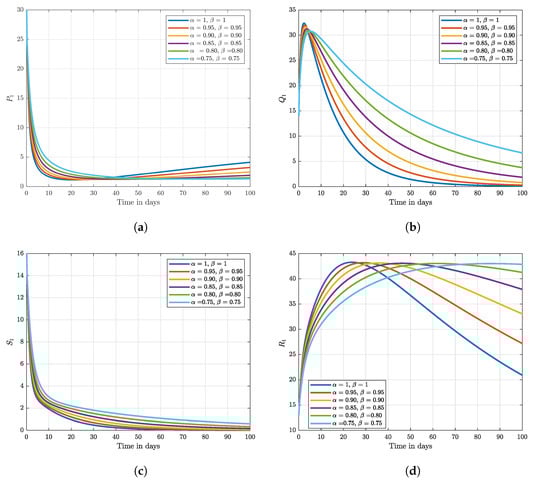
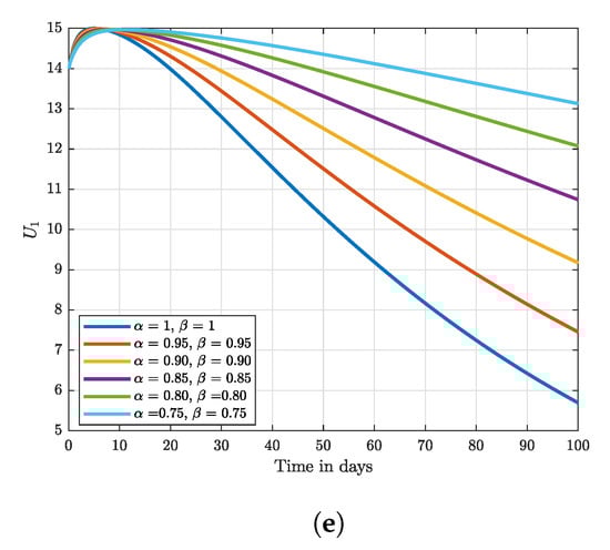
Figure 1.
Numerical smoking epidemic trajectory under the different fractal dimension and different fractional order for Group-1. (a) Dynamics of potential smokers. (b) Dynamics of occasional smokers. (c) Dynamics of the smokers class. (d) Dynamics of the smokers who temporarily quit. (e) Dynamics of the smokers who permanently quit.
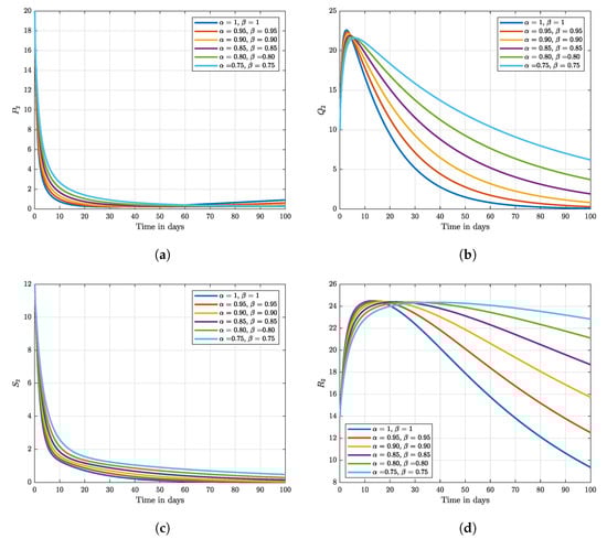
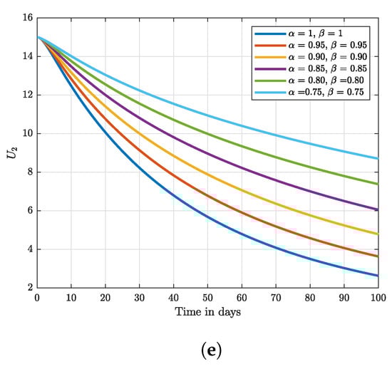
Figure 2.
Numerical smoking epidemic trajectory under the different fractal dimension and different fractional order for Group-2. (a) Dynamics of potential smokers. (b) Dynamics of occasional smokers. (c) Dynamics of the smokers class. (d) Dynamics of the smokers who temporarily quit. (e) Dynamics of the smokers who permanently quit.
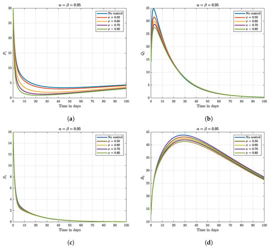
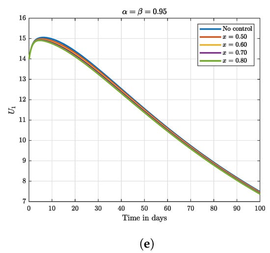
Figure 3.
Dynamics of the smoking epidemic under the CF fractal-fractional operator when the rate of government intervention varied for Group-1. (a) Dynamics of potential smokers. (b) Dynamics of occasional smokers. (c) Dynamics of the smokers class. (d) Dynamics of the smokers who temporarily quit. (e) Dynamics of the smokers who permanently quit.
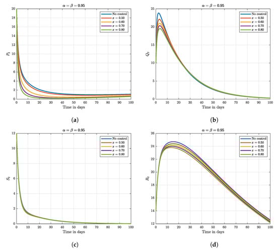
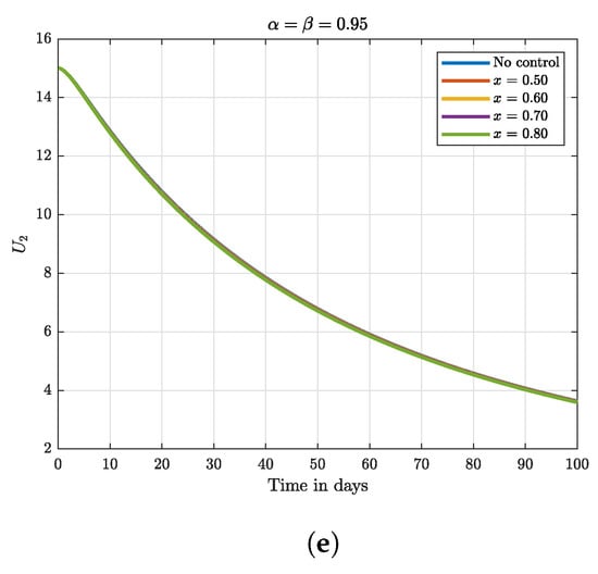
Figure 4.
Dynamics of the smoking epidemic under the CF fractal-fractional operator when the rate of government intervention varied for Group-2. (a) Dynamics of potential smokers. (b) Dynamics of occasional smokers. (c) Dynamics of the smokers class. (d) Dynamics of the smokers who temporarily quit. (e) Dynamics of the smokers who permanently quit.
9. Conclusions
In this study, we developed fractal-fractional two age-structure smoking epidemic models. The models are initially formulated via a classical integer order differential system. Then, in the rest phase, we extended to the CF fractal-fractional derivatives. The basic mathematical properties, including boundedness, positivity, and model invariance, were explored. By means of the fixed point theorem, we proved the existence and uniqueness sets of the solutions of the fractal-fractional two age-structure smoking epidemic models, and due to a small change in the initial conditions, we proved the stability solutions using the HU stability type. In the second part of the paper, the two new fractal-fractional age-structure smoking epidemic models were solved numerically using the newly built Newton polynomial, followed by numerical simulations. The graphical representation indicated the dynamics of the fractal-fractional operators and the unique dynamism of a single operator when the other operator is kept constant. To be able to control the smoking epidemic, governments and all stakeholders should implement feasible campaigns, taking into account all age groups. In the future, this work could be used to study different fractional operators and fractal-fractional optimal control.
Author Contributions
E.A.: Conceptualization, Methodology, Formal analysis, Writing—original draft, Writing—review & editing. A.A.: Methodology, Formal analysis, Writing—review & editing. O.J.P.: Formal analysis, Writing—original draft, Writing—review & editing. J.O.A.: Software, Validation, Data curation, Visualization, Writing- review & editing. K.O.: Project administration, Investigation, Funding acquisition, Supervision, Methodology, Formal analysis, Writing—review & editing. All authors have read and agreed to the published version of the manuscript.
Funding
This research received no external funding.
Data Availability Statement
Not applicable.
Conflicts of Interest
The authors declare no conflict of interest.
References
- World Health Organization Tobacco Report. Fact-Sheets about Tobacco. 2021. Available online: https://www.who.int/news-room/fact-sheets/detail/tobacco (accessed on 11 December 2022).
- World Health Organization Tobacco Report. Tobacco in the Western Pacific. 2021. Available online: https://www.who.int/westernpacific/health-topics/tobacco (accessed on 11 December 2022).
- Aslam, M.; Murtaza, R.; Abdeljawad, T.; Rahman, G.U.; Khan, A.; Khan, H.; Gulzar, H. A fractional order HIV/AIDS epidemic model with Mittag-Leffler kernel. Adv. Differ. Equ. 2021, 2021, 107. [Google Scholar] [CrossRef]
- Sher, M.; Shah, K.; Khan, Z.A.; Khan, H.; Khan, A. Computational and theoretical modeling of the transmission dynamics of novel COVID-19 under Mittag-Leffler Power Law. Alex. Eng. J. 2020, 59, 3133–3147. [Google Scholar] [CrossRef]
- Chukwu, W.; Nyabadza, F. A mathematical model and optimal control for Listeriosis disease from ready-to-eat food products. medRxiv 2020. [Google Scholar] [CrossRef]
- Osman, S.; Makinde, O.D.A. Mathematical model for co-infection of listeriosis and anthrax diseases. Int. J. Math. Math. Sci. 2018, 2018, 1725671. [Google Scholar] [CrossRef]
- Sardar, T.; Rana, S.; Bhattacharya, S.; Al-Khaled, K.; Chattopadhyay, J. A generic model for a single strain mosquito-transmitted disease with memory on the host and the vector. Math. Biosci. 2015, 263, 18–38. [Google Scholar] [CrossRef]
- Mensah, J.A.; Dontwi, I.K.; Bonyah, E. Stability analysis of Zika-malaria co-infection model for malaria endemic region. J. Adv. Math. Comput. Sci. 2018, 26, 1–22. [Google Scholar] [CrossRef]
- Peter, O.J.; Yusuf, A.; Ojo, M.M. A Mathematical Model Analysis of Meningitis with Treatment and Vaccination in Fractional Derivatives. Int. J. Appl. Comput. Math. 2022, 8, 117. [Google Scholar] [CrossRef]
- Baleanu, D.; Jajarmi, A.; Mohammad, H.; Rezapour, S. A new study on the mathematical modelling of human liver with Caputo-Fabrizio fractional derivative. Chaos Solit. Fract. 2020, 134, 109705. [Google Scholar] [CrossRef]
- Asamoah, J.K.K.; Okyere, E.; Yankson, E.; Opoku, A.A.; Adom-Konadu, A.; Acheampong, E.; Arthur, Y.D. Non-fractional and fractional mathematical analysis and simulations for Q fever. Chaos Solitons Fractals 2022, 156, 111821. [Google Scholar] [CrossRef]
- Castillo-Garsow, C.; Jordan-Salivia, G.; Rodriguez-Herrera, A. Mathematical Models for the Dynamics of Tobacco Use, Recovery, and Replase; Technical Report BU-1505-M; Cornell University: Ithaca, NY, USA, 2000. [Google Scholar]
- Zaman, G. Qualitative Behavior of Giving up Smoking Models. Bull. Malays. Math. Sci. Soc. 2011, 34, 403–415. [Google Scholar]
- Zaman, G. Optimal Campaign in the Smoking Dynamics. Comput. Math. Methods Med. 2011, 2011, 163834. [Google Scholar] [CrossRef]
- Abdullah, M.; Ahmad, A.; Raza, N.; Farman, M.; Ahmad, M. Approximate Solution and Analysis of Smoking Epidemic Model with Caputo Fractional Derivatives. Int. J. Appl. Comput. Math. 2018, 4, 112. [Google Scholar] [CrossRef]
- Khan, S.A.; Shah, K.; Zaman, G.; Jarad, F. Existence theory and numerical solutions to smoking model under Caputo-Fabrizio fractional derivative. Chaos 2019, 29, 013128. [Google Scholar] [CrossRef]
- Bonyah, E.; Yavuz, M.; Baleanu, D.; Kumar, S. A robust study on the listeriosis disease by adopting fractal-fractional operators. Alex. Eng. J. 2022, 61, 2016–2028. [Google Scholar] [CrossRef]
- Ahmad, Z.; Bonanomi, G.; di Serafino, D.; Giannino, F. Transmission dynamics and sensitivity analysis of pine wilt disease with asymptomatic carriers via fractal-fractional differential operator of Mit-tag-Leffler kernel. Appl. Numer. Math. 2023, 185, 446–465. [Google Scholar] [CrossRef]
- Malik, A.; Alkholief, M.; Aldakheel, F.M.; Ali Khan, A.; Ahmad, Z.; Kamal, W.; Khalil Gatasheh, M.; Alshamsan, A. Sensitivity analysis of COVID-19 with quarantine and vaccination: A fractal-fractional model. Alex. Eng. J. 2022, 61, 8859–8874. [Google Scholar] [CrossRef]
- Addai, E.; Zhang, L.; Asamoah, J.K.K.; Preko, A.K.; Arthur, Y.D. Fractal–fractional age-structure study of omicron SARS-CoV-2 variant transmission dynamics. Partial. Differ. Equ. Appl. Math. 2022, 6, 100455. [Google Scholar] [CrossRef]
- Addai, E.; Zhang, L.; Ackora-Prah, J.; Gordon, J.F.; Asamoah, J.K.K.; Essel, J.F. Fractal-fractional order dynamics and nu-merical simulations of a Zika epidemic model with insecticide-treated nets. Phys. A 2022, 603, 127809. [Google Scholar] [CrossRef]
- Addai, E.; Zhang, L.; Asamoah, J.K.; Essel, J.F. A fractional order age-specific smoke epidemic model. Appl. Math. Model. 2023, 119, 99–118. [Google Scholar] [CrossRef]
- Atangana, A.; Owolabi, K.M. New numerical approach for fractional differential equations. Math. Model Nat. Phenom 2018, 13, 3. [Google Scholar] [CrossRef]
- Ahmed, E.; El-Sayed, A.M.A.; El-Saka, H.A. Equilibrium points, stability and numerical solutions of fractional-order predator–prey and rabies models. J. Math. Anal. Appl. 2007, 325, 542–553. [Google Scholar] [CrossRef]
- Ritchie, H.; Roser, M. “Smoking”. 2013. Available online: https://ourworldindata.org/smoking (accessed on 11 December 2022).
- Atangana, A.; Araz, S.I. New Numerical Scheme with Newton Polynomial: Theory, Methods, and Applications; Academic Press: Cambridge, MA, USA, 2021. [Google Scholar]


Disclaimer/Publisher’s Note: The statements, opinions and data contained in all publications are solely those of the individual author(s) and contributor(s) and not of MDPI and/or the editor(s). MDPI and/or the editor(s) disclaim responsibility for any injury to people or property resulting from any ideas, methods, instructions or products referred to in the content. |
© 2023 by the authors. Licensee MDPI, Basel, Switzerland. This article is an open access article distributed under the terms and conditions of the Creative Commons Attribution (CC BY) license (https://creativecommons.org/licenses/by/4.0/).