Study Models of COVID-19 in Discrete-Time and Fractional-Order

Abstract

The novel coronavirus disease (SARS-CoV-2) has caused many infections and deaths throughout the world; the spread of the coronavirus pandemic is still ongoing and continues to affect healthcare systems and economies of countries worldwide. Mathematical models are used in many applications for infectious diseases, including forecasting outbreaks and designing containment strategies. In this paper, we study two types of SIR and SEIR models for the coronavirus. This study focuses on the discrete-time and fractional-order of these models; we study the stability of the fixed points and orbits using the Jacobian matrix and the eigenvalues and eigenvectors of each case; moreover, we estimate the parameters of the two systems in fractional order. We present a statistical study of the coronavirus model in two countries: Saudi Arabia, which has successfully recovered from the SARS-CoV-2 pandemic, and China, where the number of infections remains significantly high.

1. Introduction

Coronaviruses can infect and circulate among different animal species; the virus may spread from animals [1] (such as cats, dogs, or bats) to humans; the latest scientific research suggests that the potential scale of novel coronavirus generation in both wild and domestic animals is greater than previously thought [2,3]. New coronaviruses can emerge when two different strains co-infect an individual, causing the viral genetic material to recombine. People infected with the coronavirus have had a wide range of symptoms, according to each case, from mild symptoms to severe illness [4]. These symptoms may appear 2–14 days after exposure to the virus. Individuals can have mild to severe symptoms, which may include fever or chills [5], cough, difficulty breathing, shortness of breath, fatigue, aches and pains in the body, headaches, loss of smell or taste, flu-like symptoms, a runny or congested nose, nausea, vomiting, and diarrhea [6]. Researchers studied the evolutionary history of the coronavirus and found one strain that is responsible for it. They also discovered that the closest known ancestor of SARS-CoV-2 lived in bats 40–70 years ago [1] and then passed on to humans.

The first human coronavirus strains, HCoV-229E and HCoV-OC43, were discovered in 1966 and 1967, respectively. Since then, four other human strains have been identified: SARS-CoV in 2003, HCoV-NL63 in 2004, HCoV-HKU1 in 2005, and the MERS-CoV strain in 2012. Another was discovered in 2019: SARS-CoV-2 [7,8].

The first coronavirus outbreak occurred in Wuhan, China, in November 2019. In December 2019, China reported the first 25 cases of infected individuals in Wuhan, and then the coronavirus rapidly spread throughout China and across the world [2]. In China, the number of confirmed coronavirus cases has gradually increased, reaching 4,836,633 confirmed cases on 13 January 2023 (data sources of cases and deaths are from JHU CSSE [9]). The first coronavirus infection in Saudi Arabia [10] was identified and announced on 2 March 2020.The number of confirmed coronavirus cases has gradually grown, reaching 827,358 on 13 January 2023. (Data sources of cases and deaths are from JHU CSSE and WHO [9,11]).

Recently, mathematical models have been widely used as epidemiological tools [12,13]. They can be used to combat many infectious diseases [14]. They are methods used for studying the dynamics of infectious disease spread, including foot-and-mouth disease, and, as stated in reference [15], the flu (influenza), Hepatitis, Ebola, and coronavirus. There are many mathematical models of the coronavirus, such as the SIR, SEIR, MERS, and SARS models [12,16,17]. Epidemiological models are formulated using ordinary differential equations. However, at some point, these models cannot fully explain the natural behavior of the epidemic. The model using fractional derivatives can explain the case better.

Fractional derivatives for functions can be traced to the origin of calculus; the idea of fractional derivatives was introduced by Gottfried Wilhelm Leibniz in a letter to Guillaume de l’Hopital in the year 1695 (see [18]). The idea was further developed in the 17th century by Liouville and Riemann [19], and other types of fractional derivatives appeared. Among them, Caputo, Caputo–Fabrizio, and Atangana–Baleanu derivatives are the most important [20]. It is known that the fractional derivative of a constant is not zero, in contrast to ordinary calculus. Recently, the study of linear and nonlinear equations involving fractional derivatives brought about more interest in mathematical modeling [21].

In this paper, the authors concentrate on the SIR and SEIR systems in discrete time [22] using Euler’s method, which maintains the model and provides results over a longer time. We also study the SIR and SEIR systems using fractional calculus in discrete time, which have memory features and are useful in demonstrating many biological phenomena and facts with nonlinear dynamics behaviors. The expansion of the results obtained from the continuous-time representations of the SIR and SEIR COVID-19 systems to the fractional order in the discrete-time case [23] is clearly motivated by the general trend of using computer-assisted numerical simulations and applications, biology, and cryptography [24,25]. In the special cases of fractional order systems, estimation methods lead to new systems and expand the possibilities of representing and simulating such systems. We determine the parameters of both the SIR and SEIR models in a fractional–discrete time setting based on the registered data. We take, for example, Saudi Arabia and China [11]. Saudi Arabia is considered a leading country in combating coronavirus [11], due to the available medical services and the number of samples that were conducted for individuals. Saudi Arabia is a good example of a country where coronavirus infections have decreased. China has experienced a notable increase [9,26] compared to before.

In this paper, Section 2 provides an overview of the preliminary concepts. Section 3 highlights the SIR model, discussing its continuous-time, discrete-time, and fractional-order representations, as well as an estimation of the parameters. Section 4 focuses on the SEIR model, covering its continuous-time, discrete-time, and fractional-order formulations, using the stability of fixed points and orbits, and providing an estimation of the parameters. In Section 5, we study the coronavirus statistics in Saudi Arabia and China. Section 6 presents a discussion and the results of this study. Finally, we present the conclusions of our work.

2. Preliminaries

Definition 1. 

Let $F:[t_0,+\infty [\to \mathbb{R}$, we define the fractional order integral of a function F by

$${\displaystyle T_{t_0}^{\alpha }=\frac{1}{\mathsf{\Gamma }\left(\alpha \right)}{\int }_{t_0}^t{(t-\tau )}^{\alpha -1}d\tau .}$$

where $\alpha >0$ and $\mathsf{\Gamma }(.)$ is the gamma function.

Definition 2. 

Let $F:[t_0,+\infty [\to \mathbb{R}$, we define the Riemann–Liouville fractional derivative of F with order α by

$${\displaystyle D_{t_0}^{\alpha }F\left(t\right)=\frac{1}{\mathsf{\Gamma }(n-\alpha )}{\left(\frac{d}{dt}\right)}^n{\int }_{t_0}^t{(t-\tau )}^{n-\alpha -1}F\left(\tau \right)d\tau ,}$$

where $n\in {\mathbb{N}}^{*}$ and $n-1<\alpha <n$,

Definition 3. 

Let $F:[t_0,+\infty [\to \mathbb{R}$, we define the Caputo fractional derivative of F with order α by

$${\displaystyle {}^c{D}_{t_0}^{\alpha }F\left(t\right)=\frac{1}{\mathsf{\Gamma }(n-\alpha )}{\int }_{t_0}^t{(t-\tau )}^{n-\alpha -1}{F}^{\left(n\right)}\left(\tau \right)d\tau ,}$$

where $n\in {\mathbb{N}}^{*}$ and $n-1<\alpha <n$,

if $\alpha =n$, then ${}^c{D}_{t_0}^{\alpha }F\left(t\right)=F^{\left(n\right)}\left(t\right)$.

Let $\alpha \in (0,1)$, and consider the differential equation of the fractional order

$$\left\{\begin{array}{c}{D}^{\alpha }X\left(t\right)=F\left(X\left(t\right)\right),t>0\\ X\left(0\right)=X_0,t\le 0.\end{array}\right.$$

(1)

The corresponding equation with a piecewise constant argument is

$$\left\{\begin{array}{c}{D}^{\alpha }X\left(t\right)=F\left(X\left(a\left[\frac{t}{a}\right]\right)\right),t>0\\ X\left(0\right)=X_0,t\le 0.\end{array}\right.$$

(2)

Let $t\in [0,a)$, then $\frac{t}{a}\in [0,1)$, we find that $D^{\alpha }X\left(t\right)=F\left(X_0\right)$ we have

$$X_1\left(t\right)=X_0+\frac{t^{\alpha }}{\mathsf{\Gamma }(1+\alpha )}F\left(X_0\right)$$

and let $t\in [a,2a)$, then $\frac{t}{a}\in [1,2)$, we find that $D^{\alpha }X\left(t\right)=F\left(X_1\left(t\right)\right)$ we have

$$X_2\left(t\right)=X_1\left(a\right)+\frac{{(t-a)}^{\alpha }}{\mathsf{\Gamma }(1+\alpha )}F\left(X_1\left(a\right)\right)$$

and let $t\in [2a,3a)$, then $\frac{t}{a}\in [2,3)$, we find that $D^{\alpha }X\left(t\right)=F\left(X_2\left(t\right)\right)$ we have

$$X_3\left(t\right)=X_2\left(2a\right)+\frac{{(t-2a)}^{\alpha }}{\mathsf{\Gamma }(1+\alpha )}F\left(X_2\left(2a\right)\right).$$

By repeating the process, we find

$$D^{\alpha }X\left(t\right)=F\left(X\left(na\right)\right),t\in [na,(n+1)a)$$

we have

$$X_{n+1}\left(t\right)=X\left(na\right)+\frac{{(t-na)}^{\alpha }}{\mathsf{\Gamma }(1+\alpha )}F\left(X_n\left(na\right)\right).$$

(3)

3. SIR Model

3.1. SIR Model as a Continuous Time

In a 1927 experimental research study, Kermack and McKendrick introduced the SIR model [27]. It is a mathematical model of an infectious disease that involves three integro–differential equations that are described as follows:

$$\left\{\begin{array}{c}\frac{dS\left(t\right)}{dt}=-\frac{\beta }{N}S\left(t\right)I\left(t\right)\\ \frac{dI\left(t\right)}{dt}=\frac{\beta }{N}S\left(t\right)I\left(t\right)-\gamma I\left(t\right)\\ \frac{dR\left(t\right)}{dt}=\gamma I\left(t\right),\end{array}\right.$$

(4)

where N is the total population size, given by $N=S\left(t\right)+I\left(t\right)+R\left(t\right)$; the variables $S,I$, and R in the system represent the number of susceptible individuals, the number of infectious individuals, and the number of individuals who have been removed (recovered), respectively. A basic SIR model is shown in Figure 1, where parameter $\beta$ denotes the effective contact rate and parameter $\gamma$ denotes the mean recovery. Note that the parameters $\beta ,\gamma$ are positive real numbers, and the natural birth and death rates are ignored.

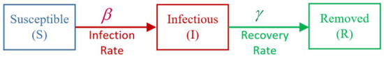
Figure 1. Basic assumptions of the SIR model.

In this case, we find that with $\beta =0.00000265$ and $\gamma =1$, and $S\left(0\right)=1,000,000,I\left(0\right)=100$ (which implies $R\left(0\right)=0$), the error between the predicted and the observed values of R is minimum; see Figure 2.

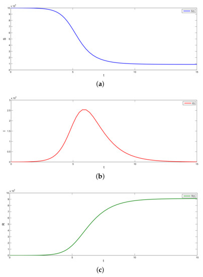
Figure 2. (a–c) Graphs of the SIR model.

Remark 1. 

The experiment was conducted on an isolated susceptible population at the beginning of the epidemic. The rate constants that define the spread of the virus are $\beta =0.00000265$ and $\gamma =1$, and are determined on a daily basis; see [28].

3.2. SIR Model as a Discrete Time

To find the discrete SIR model, we use the Euler forward-shift operator method [14]; we use equation

$$\frac{dX\left(t\right)}{dt}=\frac{X(n+1)-X\left(n\right)}{h},$$

(5)

where X is a generic signal that can be replaced by either $S,I$, or R; h is the integration step (small real number); and n is the sampling number. The discretization of the system (4) takes the following form using the approximation in Equation (5):

$$\left\{\begin{array}{c}S(n+1)=-h\frac{\beta }{N}S\left(n\right)I\left(n\right)+S\left(n\right)\\ I(n+1)=h(\frac{\beta }{N}S\left(n\right)I\left(n\right)-\gamma I\left(n\right))+I\left(n\right)\\ R(n+1)=h\gamma I\left(n\right)+R\left(n\right),\end{array}\right.$$

(6)

we use the following initial conditions:

$$S\left(0\right)\ge 0,I\left(0\right)\ge 0,R\left(0\right)\ge 0.$$

The first two equations in the proposed system (6) are unrelated to class R, and this class can be studied independently using the equation:

$$N\left(n\right)=S\left(n\right)+I\left(n\right)+R\left(n\right),$$

where N is the total population number in the hundreds of thousands or more.

3.3. Fixed Points

By equating the left-hand side equations of the proposed system (6) to $S\left(n\right),I\left(n\right)$, and $R\left(n\right)$, respectively, we obtain $R(n+1)=R\left(n\right)\Rightarrow I=0$. As a result, the discrete SIR system (6) has fixed points described by

$$S_f\in [0,N],I_f=0,R_f=N-S.$$

These fixed points indicate disease-free conditions. When applied to coronavirus epidemics that occurred at the beginning of the 2019 pandemic, the fixed point is

$$S_f=N,I_f=0,R_f=0$$

(7)

At the beginning of the pandemic in 2019, the coronavirus was a novel disease. The number of infections was not well known prior to 2019; while considering a specific population of N people, all of them were susceptible to the coronavirus. $S_f=N$. A coronavirus outbreak that starts at an initial time $n_0$ is defined as a perturbation that represents a small population of infectious people. $I\left(n_0\right)>0$, and as a result, it leads to a movement of disease cases (or individuals in a healthy state), represented by X, away from the disease-free fixed point (7). The initial conditions ($S_0=S\left(n_0\right),I_0=I\left(n_0\right)$, and $R_0=R\left(n_0\right)$) of a coronavirus epidemic that occurred at time $n_0$ are given in terms of a perturbed fixed point of the condition:

$$S_0=N-I_0,I_0\mathrm{is}\mathrm{small}\mathrm{and}{R}_0=0.$$

(8)

Actually, N is usually very large compared to $I_0$ (for example, $N=10,000,000$, and $I_0=1$), such that

$$\frac{S_0}{N}\simeq 1.$$

System (6) has fixed points on the S-axis with $S_f\le N$, which are the disease-free fixed points and initial disease states.

3.4. Orbits

Orbits can be used to visualize discrete SIR system solutions. $S\left(n\right),I\left(n\right)$, and $R\left(n\right)$. Let us write the evolution Equation (6) as follows:

$$I(n+1)=Y\left(n\right)I\left(n\right),$$

(9)

where $Y\left(n\right)=h(\frac{\beta }{N}S\left(n\right)-\gamma )+1$, and if $Y\left(n\right)=1$ at the beginning $n_0$ or at any other time point $n_c>n_0$

Hence, there are two types of $I\left(n\right)$ orbits. They describe either a monotone or non-monotone function. If it is a non-monotone function, then $I\left(n\right)$ increases gradually and reaches a peak at $n_c>n_0$, where $Y=1$ holds; after that, it decays to zero. To distinguish between these two cases, the expression $Y\left(n\right)$ for $n=n_0$ can be written as $Y=\gamma h(\rho -1)+1,$ where

$$\rho =\frac{\beta }{N\gamma }S\left(0\right),$$

(10)

where the stability parameter is indicated with $\rho$.

Figure 3 and Figure 4 represents $I\left(n\right)$ solutions for two qualitatively distinct cases. $\rho >1$ and $\rho \le 1$, for $\rho >1$, there is a wave of an epidemic. In system (6), the stability parameter $\rho$ is critical for solutions, and the epidemic under study decays monotonically for $\rho \le 1$.

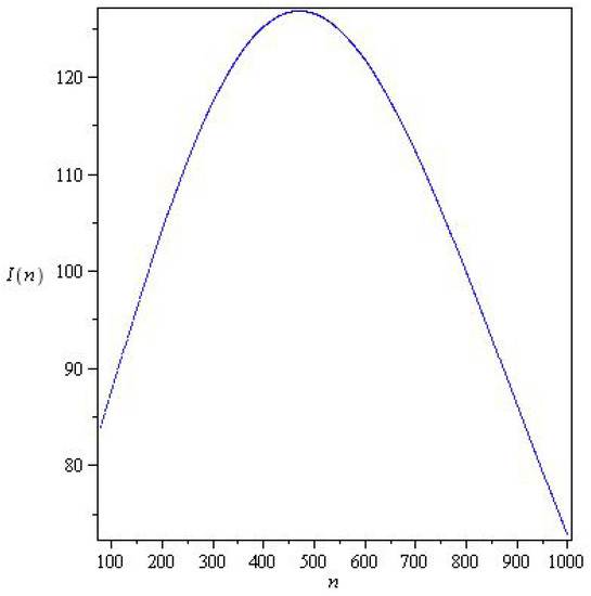
Figure 3. Solutions $I\left(n\right)$ of system (6) for $\rho >1$ with parameters $\beta =0.8$, $\gamma =0.5$, $h=0.01$, $N=1,000$ and initial conditions $\left(S\right(0),I(0),R(0\left)\right)=(930,70,20)$.

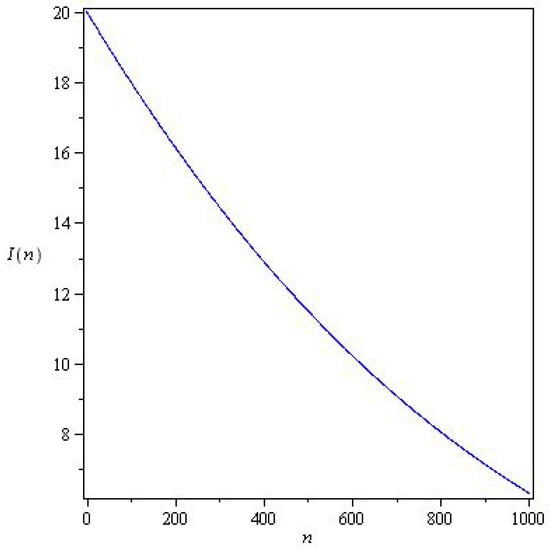
Figure 4. Solutions $I\left(n\right)$ of system (6) for $\rho \le 1$ with parameters $\beta =0.4$, $\gamma =0.5$, $h=0.01$, $N=1,000$ and initial conditions $\left(S\right(0),I(0),R(0\left)\right)=(990,20,20)$.

3.5. Stability Analysis for the Discrete Sir System

The Jacobian matrix of system (6) is given by

$$J(S_c,I_c,R_c)=\left(\begin{array}{ccc}-\frac{\beta I_{c}h}{N}+1& -\frac{\beta S_{c}h}{N}& 0\\ \frac{\beta I_{c}h}{N}& \frac{\beta S_{c}h}{N}-\gamma h+1& 0\\ 0& \gamma h& 1\end{array}\right).$$

(11)

The eigenvalues of matrix (11) are given by

$$\begin{array}{c}{\lambda }_1=1\\ {\lambda }_2=1+\frac{1}{2}h(\beta \frac{(S_c-I_c)}{N}-\gamma -\frac{1}{N}\sqrt{\mathsf{\Delta }})\\ {\lambda }_3=1+\frac{1}{2}h(\beta \frac{(S_c-I_c)}{N}-\gamma +\frac{1}{N}\sqrt{\mathsf{\Delta }}),\end{array}$$

(12)

where

$$\mathsf{\Delta }={\beta }^2{S_c}^2-2\beta S_c\gamma N-2{\beta }^2{S}_c{I}_c+{\gamma }^2{N}^2-2\gamma N\beta I_c+{\beta }^2{I_c}^2,$$

and the eigenvalues (12) evaluated at $I_f=0$ are given by

$$\begin{array}{c}{\lambda }_1={\lambda }_3=1\\ {\lambda }_2=1+h(\frac{\beta S_f}{N}-\gamma ).\end{array}$$

(13)

to find all the eigenvectors of ${\lambda }_1={\lambda }_3=1$, we need to solve $v=\left(\begin{array}{c}{x}_1\\ x_2\\ x_3\end{array}\right)$ from:

$$\left(\begin{array}{ccc}0& -\frac{\beta S_{f}h}{N}& 0\\ 0& \frac{\beta S_{f}h}{N}-\gamma h& 0\\ 0& \gamma h& 0\end{array}\right)\left(\begin{array}{c}{x}_1\\ x_2\\ x_3\end{array}\right)=\left(\begin{array}{c}0\\ 0\\ 0\end{array}\right).$$

(14)

The eigenvectors to the above equation are $v_1=\left(\begin{array}{c}1\\ 0\\ 0\end{array}\right)$ and $v_3=\left(\begin{array}{c}0\\ 0\\ 1\end{array}\right).$

For calculating the eigenvector associated with the eigenvalue ${\lambda }_2=1+h(\frac{\beta S_f}{N}-\gamma )$, we need to solve $v_3=\left(\begin{array}{c}{y}_1\\ y_2\\ y_3\end{array}\right)$ from:

$$\left(\begin{array}{ccc}h(\frac{\beta S_f}{N}-\gamma )& -\frac{\beta S_{f}h}{N}& 0\\ 0& 0& 0\\ 0& \gamma h& h(\frac{\beta S_f}{N}-\gamma )\end{array}\right)\left(\begin{array}{c}{y}_1\\ y_2\\ y_3\end{array}\right)=\left(\begin{array}{c}0\\ 0\\ 0\end{array}\right).$$

(15)

The eigenvector ${\lambda }_2$ is $v_2=\left(\begin{array}{c}-\frac{\beta S_f}{\gamma N}\\ \frac{\beta S_f}{\gamma N}-1\\ 1\end{array}\right).$

In Figure 5, the phase curves originate at states slightly above the S-axis. Consequently, the states can be changed along the two axes; for example, the fixed point $(S_f=1000,R_f=0)$ can be changed to $(S_f=998,R_f=2)$. The fixed points are not asymptotically stable, either in the form of unstable fixed points or neutrally stable fixed points. Figure 6, show wave-like solution of the SIR model (6) presented in terms of the orbitals $S\left(n\right)$ and $I\left(n\right)$. The arrows indicate the direction of the orbitals.

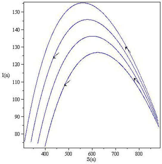
Figure 5. Phase portraits of the discrete SIR system (6) in the $(S,I)$ plane for $\beta >\gamma$ with $\gamma =0.5$ and $N=1000$.

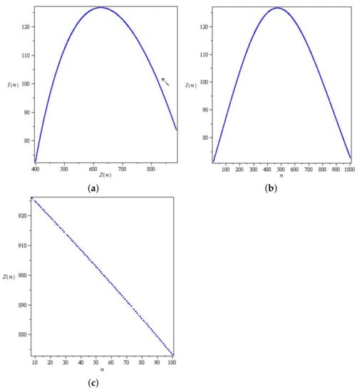
Figure 6. Wave-like solution of the SIR model (6) presented in terms of the orbitals $S\left(n\right)$ and $I\left(n\right)$. (a,b) The phase curve of $I\left(n\right)$. (c) The phase curve of $S\left(n\right)$.

3.6. Fractional-Order SIR System and Discretization

The fractional-order SIR system is given by

$$\left\{\begin{array}{c}{D}^{\alpha }S\left(t\right)=S\left(t\right)(1-\frac{\beta }{N}I\left(t\right))\\ D^{\alpha }I\left(t\right)=I\left(t\right)(\frac{\beta }{N}S\left(t\right)-\gamma +1)\\ D^{\alpha }R\left(t\right)=R\left(t\right)+\gamma I\left(t\right),\end{array}\right.$$

(16)

where $\alpha$ is the fractional order. The discretization fractional order of the SIR system [29] is given as

$$\left\{\begin{array}{c}{D}^{\alpha }S\left(t\right)=S\left(a\left[\frac{t}{a}\right]\right)(1-\frac{\beta }{N}I\left(a\left[\frac{t}{a}\right]\right))\\ D^{\alpha }I\left(t\right)=I\left(a\left[\frac{t}{a}\right]\right)(1+\frac{\beta }{N}S\left(a\left[\frac{t}{a}\right]\right)-\gamma )\\ D^{\alpha }R\left(t\right)=R\left(a\left[\frac{t}{a}\right]\right)+\gamma I\left(a\left[\frac{t}{a}\right]\right),\end{array}\right.$$

(17)

where $(S\left(0\right),I\left(0\right),R\left(0\right))=(S_0,I_0,R_0)$ are initial conditions.

The discretization method is given by the following steps.

Step 1. Let $t\in [0,a)$, then $\frac{t}{a}\in [0,1)$. Thus, we obtain

$$\left\{\begin{array}{c}{D}^{\alpha }S\left(t\right)=S_0(1-\frac{\beta }{N}{I}_0)\\ D^{\alpha }I\left(t\right)=I_0(1+\frac{\beta }{N}{S}_0-\gamma )\\ D^{\alpha }R\left(t\right)=R_0+\gamma I_0,\end{array}\right.$$

(18)

and the solution of (17) is given by

$$\left\{\begin{array}{c}{S}_1\left(t\right)=S_0+T^{\alpha }{S}_0(1-\frac{\beta }{N}{I}_0)\\ I_1\left(t\right)=I_0+T^{\alpha }{I}_0(1+\frac{\beta }{N}{S}_0-\gamma )\\ R_1\left(t\right)=R_0+T^{\alpha }(R_0+\gamma I_0).\end{array}\right.$$

(19)

Then

$$\left\{\begin{array}{c}{S}_1\left(t\right)=S_0+\frac{t^{\alpha }}{\mathsf{\Gamma }(1+\alpha )}{S}_0(1-\frac{\beta }{N}{I}_0)\\ I_1\left(t\right)=I_0+\frac{t^{\alpha }}{\mathsf{\Gamma }(1+\alpha )}{I}_0(1+\frac{\beta }{N}{S}_0-\gamma )\\ R_1\left(t\right)=R_0+\frac{t^{\alpha }}{\mathsf{\Gamma }(1+\alpha )}(R_0+\gamma I_0),\end{array}\right.$$

(20)

Step 2. Let $t\in [a,2a)$ then $\frac{t}{a}\in [a,2a)$. Thus, we obtain

$$\left\{\begin{array}{c}{D}^{\alpha }S\left(t\right)=S_1(1-\frac{\beta }{N}{I}_1)\\ D^{\alpha }I\left(t\right)=I_1(1+\frac{\beta }{N}{S}_1-\gamma )\\ D^{\alpha }R\left(t\right)=R_1+\gamma I_1,\end{array}\right.$$

(21)

and the solution of (17) is given by

$$\left\{\begin{array}{c}{S}_2\left(t\right)=S_1+T^{\alpha }{S}_1(1-\frac{\beta }{N}{I}_1)\\ I_2\left(t\right)=I_1+T^{\alpha }{I}_1(1+\frac{\beta }{N}{S}_1-\gamma )\\ R_2\left(t\right)=R_1+T^{\alpha }(R_1+\gamma I_1),\end{array}\right.$$

(22)

Then

$$\left\{\begin{array}{c}{S}_2\left(t\right)=S_1+\frac{t^{\alpha }}{\mathsf{\Gamma }(1+\alpha )}{S}_1(1-\frac{\beta }{N}{I}_1)\\ I_2\left(t\right)=I_1+\frac{t^{\alpha }}{\mathsf{\Gamma }(1+\alpha )}{I}_1(1+\frac{\beta }{N}{S}_1-\gamma )\\ R_2\left(t\right)=R_1+\frac{t^{\alpha }}{\mathsf{\Gamma }(1+\alpha )}(R_1+\gamma I_1).\end{array}\right.$$

(23)

Step 3. We repeat the process to find the solution to (17) as

$$\left\{\begin{array}{c}{S}_{n+1}\left(t\right)=S_n\left(na\right)+\frac{{(t-na)}^{\alpha }}{\mathsf{\Gamma }(1+\alpha )}{S}_n\left(na\right)(1-\frac{\beta }{N}{I}_n\left(na\right))\\ I_{n+1}\left(t\right)=I_n\left(na\right)+\frac{{(t-na)}^{\alpha }}{\mathsf{\Gamma }(1+\alpha )}{I}_n\left(na\right)(1+\frac{\beta }{N}{S}_n\left(na\right)-\gamma )\\ R_{n+1}\left(t\right)=R_n\left(na\right)+\frac{{(t-na)}^{\alpha }}{\mathsf{\Gamma }(1+\alpha )}(R_n\left(na\right)+\gamma I_n\left(na\right)).\end{array}\right.$$

(24)

We assume that $t\to (n+1)a$; then we have the following discretization

$$\left\{\begin{array}{c}{S}_{n+1}\left((n+1)a\right)=S_n\left(na\right)+\frac{a^{\alpha }}{\mathsf{\Gamma }(1+\alpha )}{S}_n\left(na\right)(1-\frac{\beta }{N}{I}_n\left(na\right))\\ I_{n+1}\left((n+1)a\right)=I_n\left(na\right)+\frac{a^{\alpha }}{\mathsf{\Gamma }(1+\alpha )}{I}_n\left(na\right)(1+\frac{\beta }{N}{S}_n\left(na\right)-\gamma )\\ R_{n+1}\left((n+1)a\right)=R_n\left(na\right)+\frac{a^{\alpha }}{\mathsf{\Gamma }(1+\alpha )}(R_n\left(na\right)+\gamma I_n\left(na\right)),\end{array}\right.$$

(25)

which can be expressed as

$$\left\{\begin{array}{c}{S}_{n+1}=S_n+\frac{a^{\alpha }}{\mathsf{\Gamma }(1+\alpha )}{S}_n(1-\frac{\beta }{N}{I}_n)\\ I_{n+1}=I_n+\frac{a^{\alpha }}{\mathsf{\Gamma }(1+\alpha )}{I}_n(1+\frac{\beta }{N}{S}_n-\gamma )\\ R_{n+1}=R_n+\frac{a^{\alpha }}{\mathsf{\Gamma }(1+\alpha )}(R_n+\gamma I_n).\end{array}\right.$$

(26)

3.7. Fixed Points and Stability

System (26) has two fixed points, which are given as:

$$M_0(0,0,0);M_1\left(\frac{(\gamma -1)N}{\beta },\frac{N}{\beta },\frac{-\gamma N}{\beta }\right).$$

At a fixed point $M_0(0,0,0)$, the Jacobian matrix of system (26) is given by

$$J\left(M_0\right)=\left(\begin{array}{ccc}\theta +1& 0& 0\\ 0& \left(1-\gamma \right)\theta +1& 0\\ 0& \gamma \theta & \theta +1\end{array}\right),$$

where $\theta =\frac{a^{\alpha }}{\mathsf{\Gamma }(1+\alpha )}$, and the eigenvalues of matrix $J\left(M_0\right)$ are given as follows

$${\lambda }_1={\lambda }_2=\theta +1,{\lambda }_3=\left(1-\gamma \right)\theta +1,$$

then ${\lambda }_1,{\lambda }_2$, and ${\lambda }_3$ are real eigenvalues and $|{\lambda }_i|>1$, $i=1,2$.

Theorem 1. 

Let $|{\lambda }_i|>1$, $i=1,2$.

• If $\gamma <1$ or $\gamma >\frac{2}{\theta }$, then $\mid {\lambda }_3\mid >1$, and the fixed point $M_0$ is an unstable node.
• If $\gamma >1$ or $\gamma <\frac{2}{\theta }$, then $\mid {\lambda }_3\mid <1$ and the fixed point $M_0$ is a saddle.

At the fixed point $M_1\left(\frac{(\gamma -1)N}{\beta },\frac{N}{\beta },\frac{-\gamma N}{\beta }\right)$, the Jacobian matrix of system (26) is given by

$$J\left(M_1\right)=\left(\begin{array}{ccc}1& \frac{\left(1-\gamma \right)\theta }{N}& 0\\ \theta & \left(\frac{\gamma -1}{N}-\gamma +1\right)\theta +1& 0\\ 0& \gamma \theta & \theta +1\end{array}\right),$$

where $\theta =\frac{a^{\alpha }}{\mathsf{\Gamma }(1+\alpha )}$, and the eigenvalues of $J\left(M_1\right)$ are solutions of the following equation

$$P\left(\lambda \right)=(\lambda -1-\theta )(A_2{\lambda }^2+A_1\lambda +A_0),$$

where $A_0=\frac{\gamma \theta +\theta N-\theta +{\theta }^2\gamma +N-\theta \gamma N-{\theta }^2}{N}$

$A_1=\frac{\left(-\theta N+\theta \gamma N-\gamma \theta -2N+\theta \right)}{N}.$

The eigenvalues of matrix $J\left(M_1\right)$ are given by

$$\begin{array}{c}{\lambda }_1=\theta +1\\ {\lambda }_2=\frac{\theta N-\theta \gamma N+\gamma \theta +2N-\theta +\sqrt{\omega }}{2N}\\ {\lambda }_3=\frac{\theta N-\theta \gamma N+\gamma \theta +2N-\theta -\sqrt{\omega }}{2N}\end{array},$$

where

$$\omega =2{\theta }^{2}N+{\theta }^2+{\theta }^2{\gamma }^2{N}^2-2{\theta }^2{N}^2\gamma +{\theta }^2{N}^2+{\theta }^2{\gamma }^2-2{\theta }^2\gamma -2{\theta }^2{\gamma }^{2}N.$$

Theorem 2. 

Let ${\lambda }_1=\theta +1$. Then, if $\mid {\lambda }_1\mid >1$, and

if $\omega >0$, we have ${\lambda }_2$ and ${\lambda }_3$ as real eigenvalues; we obtain the following

• If $\mid {\lambda }_2\mid >1$ and $\mid {\lambda }_3\mid >1$, then the fixed point $M_1$ is an unstable node.
• If $\mid {\lambda }_2\mid <1$ and $\mid {\lambda }_3\mid <1$, then the fixed point $M_1$ is a saddle.

If $\omega <0$, then ${\lambda }_2$ and ${\lambda }_3$ are complex conjugate eigenvalues; we obtain:

• If $\mid {\lambda }_2\mid >1$ and $\mid {\lambda }_3\mid >1$, then the fixed point $M_1$ is an unstable spiral node.
• If $\mid {\lambda }_2\mid <1$ and $\mid {\lambda }_3\mid <1$, then the fixed point $M_1$ is a saddle-spiral.

3.8. Determining $\beta$ and $\gamma$ for Model (26) at a Discrete Time from the Observed Data

In this study, the algorithm proposed in [30,31] was used to estimate the fractional–discrete-time SIR model parameters and the method used to predict coronavirus cases in China and Saudi Arabia. The parameters $\beta$ and $\gamma$ are determined from the following equations in discrete time:

$$\left\{\begin{array}{c}\frac{S_{n+1}-S_n}{\theta \left(n\right)}=S_n(1-\frac{\beta \left(n\right)}{N}{I}_n)\\ \frac{I_{n+1}-I_n}{\theta \left(n\right)}=I_n(1+\frac{\beta \left(n\right)}{N}{S}_n-\gamma \left(n\right))\\ \frac{R_{n+1}-R_n}{\theta \left(n\right)}=(R_n+\gamma \left(n\right)I_n),\end{array}\right.$$

(27)

where $\theta \left(n\right)=\frac{a^{\alpha }}{\mathsf{\Gamma }(1+\alpha )}$, and $n-1<\alpha <n$, for example, if $\alpha =\frac{1}{2}$, then $\theta \left(n\right)=\frac{1}{2^{n-1}\sqrt{\pi }}$, and if $\alpha =\frac{1}{2}$ then $\theta \left(n\right)=\frac{1}{3.2^{n-2}\sqrt{\pi }}$. We note that if n is a large value, then $\theta \left(n\right)$ takes a small value $0<\theta \left(n\right)<1$. In this study, we choose $\theta =0.01$.

From Equations (27), we have

$$\beta \left(n\right)=\frac{N((1+\theta \left(n\right))S_n-S_{n+1})}{S_n{I}_n\theta \left(n\right)},$$

(28)

and

$$\gamma \left(n\right)=\frac{N(R_{n+1}-(1+\theta \left(n\right))R_n)}{I_n\theta \left(n\right)}.$$

(29)

In this study we assume that the SIR model in Saudi Arabia depends on an exponential decay function written in the following form.

$$\beta \left(t\right)={\beta }_1{exp}^{-{\beta }_{2}t},$$

(30)

and

$$\gamma \left(t\right)=\gamma \left(n\right),$$

(31)

where ${\beta }_1,{\beta }_1\in {\mathbb{R}}_{+}^{*}$, $\gamma \in {\mathbb{R}}_{+}$ and $t\ge 1$. Using the logarithm in Equation (30), we find

$$ln\left(\beta \left(t\right)\right)=ln\left({\beta }_1\right)-{\beta }_{2}t,$$

(32)

By placing ${\rho }_1=ln\left({\beta }_1\right)$ and ${\rho }_2=-{\beta }_2$ in Equation (32), we have

$$ln\left(\beta \left(t\right)\right)={\rho }_1+{\rho }_{2}t.$$

(33)

using the maximum log-likelihood estimation (MLE) method in [32,33]. MLEs draw conclusions from the observed data, particularly the joint probability distribution (see [34]) of the random variables $(x_1,x_2,...,x_n)$. To find suitable estimators $\widetilde{{\beta }_1},\widetilde{{\beta }_2}$ and $\tilde{\gamma }$ for ${\beta }_1$, ${\beta }_2$, and $\gamma$, respectively. We define the positive cost function as follows

$${\displaystyle \mathsf{\Phi }({\rho }_1,{\rho }_2,\gamma )={\mathsf{\Sigma }}_{i=2}^K({\rho }_1+{\rho }_2{t}_i-ln{\left({\beta }_i\right)}^2)+{\mathsf{\Sigma }}_{i=2}^K(\gamma -{\gamma }_i).}$$

(34)

The solutions of Equation (34) are called local minimizers $\widetilde{{\rho }_1},\widetilde{{\rho }_2}$ and $\tilde{\gamma }$, which can be obtained by the following method

$$\frac{\partial \mathsf{\Phi }(\widetilde{{\rho }_1},\widetilde{{\rho }_2},\tilde{\gamma })}{\partial {\rho }_1}=\frac{\partial \mathsf{\Phi }(\widetilde{{\rho }_1},\widetilde{{\rho }_2},\tilde{\gamma })}{\partial {\rho }_2}=\frac{\partial \mathsf{\Phi }(\widetilde{{\rho }_1},\widetilde{{\rho }_2},\tilde{\gamma })}{\partial \gamma }=0.$$

(35)

Simplifying the equations given in (35), we have

$${\displaystyle \tilde{\gamma }=\frac{1}{K-1}{\mathsf{\Sigma }}_{i=2}^K{\gamma }_i.}$$

(36)

$${\displaystyle \widetilde{{\rho }_1}=\frac{1}{K-1}{\mathsf{\Sigma }}_{i=2}^K(ln{\beta }_i-t_i\widetilde{{\rho }_2}),}$$

(37)

where $\widetilde{{\rho }_2}$, given by

$$\widetilde{{\rho }_2}=\frac{{\mathsf{\Sigma }}_{i=2}^K{t}_i.ln{\beta }_i-\frac{1}{K-1}\left({\mathsf{\Sigma }}_{i=2}^{K}ln{\beta }_i\right).{\mathsf{\Sigma }}_{i=2}^K{t}_i}{{\mathsf{\Sigma }}_{i=2}^K{t}_i^2-\frac{1}{K-1}.{\left({\mathsf{\Sigma }}_{i=2}^K{t}_i\right)}^2}.$$

(38)

Hence, using these parameters $(\tilde{\gamma },\widetilde{{\rho }_1},\widetilde{{\rho }_2})$ we estimate the values of (30) and (31) with a relative mean absolute error (see [35,36]), which can be calculated by

$${\displaystyle ϵ=\frac{1}{N}{\mathsf{\Sigma }}_{i=1}^N\frac{|x_i-p_i|}{x_i}}$$

(39)

where $x\left(i\right)$ denotes the observed state, $q\left(i\right)$ denotes the simulated state of $\tilde{\gamma }$, and $\tilde{\delta }$ and N denote the sizes of sampled data. The correlation coefficient (see [36]), produced by the equation, can be used to confirm the accuracy of the results for the three parameters.

$$\epsilon =\sqrt{1-\frac{{\mathsf{\Sigma }}_{i=1}^N(x_i-p_i^2)}{{\mathsf{\Sigma }}_{i=1}^N{(x_i-\overline{x})}^2}},$$

(40)

the best value of the correlation coefficient is given if $\epsilon \in [-1,1]$.

4. SEIR Model

4.1. SEIR Model as a Continuous Time

It is important to know that the coronavirus disease has an incubation period, which is the time between the virus exposure and the onset of symptoms. The average incubation period is 5–6 days but can last up to 14 days. The SIR model described in (4) does not provide information about the exposed individuals who are infected but have not been detected yet (infected but still not infectious). It does not provide any information about closed cases of infectious people who have died. To write the SEIR model, an exposed variable E can be added to the SIR model [12]. The differential equations of this model are as follows:

$$\left\{\begin{array}{c}\frac{dS\left(t\right)}{dt}=-\frac{\beta }{N}S\left(t\right)I\left(t\right)\\ \frac{dE\left(t\right)}{dt}=\frac{\beta }{N}S\left(t\right)I\left(t\right)-\delta E\left(t\right)\\ \frac{dI\left(t\right)}{dt}=\delta E\left(t\right)-\gamma I\left(t\right)\\ \frac{dR\left(t\right)}{dt}=\gamma I\left(t\right),\end{array}\right.$$

(41)

where E denotes the exposed state variable, $\delta$ denotes the exposed parameter, $\gamma$ denotes the dead variable, and the total population is denoted by $N=S\left(t\right)+E\left(t\right)+I\left(t\right)+R\left(t\right)$. Figure 7 present the basic assumptions of the SEIR model.

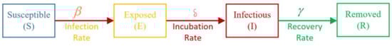
Figure 7. Basic assumptions of the SEIR model.

Figure 8 was obtained with fixed parameters $\beta =0.00000265,\gamma =1$, $\delta =0.5$ and initial conditions $S_0=1000000,E_0=0,I_0=100,R_0=0.$

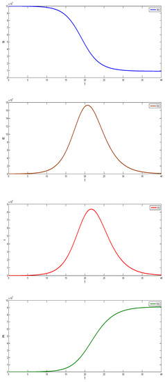
Figure 8. Graphs of the SEIR model.

Remark 2. 

Parameters $\beta =0.00000265$, $\gamma =1$, and $\gamma =0.5$ are determined in the same method, i.e., experimentally on a non-isolated population, and the results are taken on a daily basis; see [28,37].

4.2. SEIR Model as a Discrete Time

To find the SEIR discrete system, we use the Euler forward-shift operator method, and write

$$\frac{dZ\left(t\right)}{dt}=\frac{Z(n+1)-Z\left(n\right)}{h},$$

(42)

where Z can be changed by any variable $S,E,I$, or R; h takes a small value, and n is an integer. The SEIR discrete system for Equation (41) takes the following form when applied to the approximation in Equation (42):

$$\left\{\begin{array}{c}S(n+1)=-h\frac{\beta }{N}S\left(n\right)I\left(n\right)+S\left(n\right)\\ E(n+1)=h(\frac{\beta }{N}S\left(n\right)I\left(n\right)-\delta E\left(n\right))+E\left(n\right)\\ I(n+1)=h\left(\delta E\right(n)-\gamma I(n\left)\right)+I\left(n\right)\\ R(n+1)=h\gamma I\left(n\right)+R\left(n\right),\end{array}\right.$$

(43)

where $S\left(0\right)\ge 0,E\left(0\right)\ge 0,I\left(0\right)\ge 0,R\left(0\right)\ge 0$.

4.3. Fixed Points

The fixed points of a system (43) are the roots of the equation vector $Z(n+1)=Z\left(n\right)$. We can find the fixed points by solving this equation. The fixed points of (43) are given by

$$S_f\in [0,N],E_f=0,I_f=0\mathrm{and}{R}_f=N-S_f.$$

(44)

Linearizing system (43) of the fixed point, we can find the eigenvalues of the Jacobian matrix; these eigenvalues will determine the nature of the fixed point, with fixed $N=N_0$. The Jacobian matrix at a fixed point is as follows

$$J(S_f,E_f,I_f,R_f)=\left(\begin{array}{cccc}-\frac{h\beta I_f}{N_0}+1& 0& -\frac{h\beta S_f}{N_0}& 0\\ \frac{h\beta I_f}{N_0}& -h\delta +1& \frac{h\beta S_f}{N_0}& 0\\ 0& h\delta & -h\gamma +1& 0\\ 0& 0& h\gamma & 1\end{array}\right).$$

(45)

Evaluating (45) at $I_f=0$, we find the following matrix

$$J(S_f,0,0,N-S_f)=\left(\begin{array}{cccc}1& 0& -\frac{h\beta S_f}{N}& 0\\ 0& -h\delta +1& \frac{h\beta S_f}{N}& 0\\ 0& h\delta & -h\gamma +1& 0\\ 0& 0& h\gamma & 1\end{array}\right).$$

(46)

The eigenvalues of this matrix are given by

$$\begin{array}{c}{\lambda }_2=1-\frac{h}{2}\gamma -\frac{h}{2}\delta +\frac{h}{2}\sqrt{\mathsf{\Delta }}\\ {\lambda }_3=1-\frac{h}{2}\gamma -\frac{h}{2}\delta -\frac{h}{2}\sqrt{\mathsf{\Delta }}\\ {\lambda }_1={\lambda }_4=1,\end{array}$$

(47)

$$\mathsf{\Delta }={(\gamma -\delta )}^2+4\frac{\delta \beta S}{N}>0,$$

Theorem 3. 

Let ${\lambda }_1={\lambda }_4=1$; if $|{\lambda }_2|<1$ and $|{\lambda }_3|<1$, the fixed points are stable. If $|{\lambda }_2|>1$ or ${\lambda }_3>1$. We use the following numerical study to prove that the fixed points are unstable.

Let ${\lambda }_1={\lambda }_4=1$; if $|{\lambda }_2|<1$ and $|{\lambda }_3|<1$, the fixed points are stable. If $|{\lambda }_2|>1$ or $|{\lambda }_3|>1$. We use the following numerical study to prove that the fixed points are unstable.

Figure 9 and Figure 10 show two types of curves for the discrete SEIR system. Figure 9 exemplifies the case $\beta >\gamma$ of the parameters, and the initial conditions chosen $R\left(n\right)$ are initially increasing. However, $S\left(n\right)$ decays over time, while $E\left(n\right)$ and $I\left(n\right)$ increase until they reach maximum values and then decrease. Figure 10 exemplifies the case $\beta <\gamma$ for the parameters, and the initial conditions chosen $R\left(n\right)$ are initially increasing. However, $S\left(n\right)$ and $E\left(n\right)$ decay over time, while $I\left(n\right)$ increases until it reaches the maximum value and then decreases.

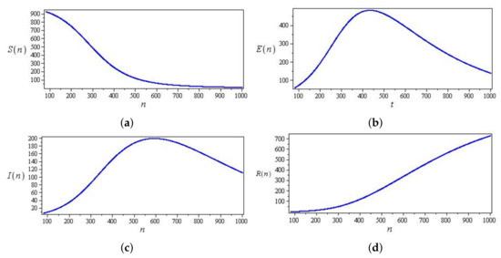
Figure 9. Phase curves of a discrete SEIR system (43) with parameters $\beta =1.5, \gamma =0.6$, $N=1000$, and $\delta =0.3, h=0.01$, and initial conditions $S\left(0\right)=975, E\left(0\right)=25, I\left(0\right)=0$ and $R\left(0\right)=0$ (a) Curve in $(n,S(n\left)\right)$-plane (b) Curve in $(n,E(n\left)\right)$-plane (c) Curve in $(n,I(n\left)\right)$-plane (d) Curve in $(n,R(n\left)\right)$-plane.

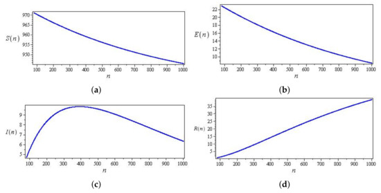
Figure 10. Curves of the discrete SEIR system (43) with parameters $\beta =0.2, \gamma =0.5$, $N=1000$, and $\delta =0.3, h=0.01$, and initial conditions $S\left(0\right)=975, E\left(0\right)=25, I\left(0\right)=0$, and $R\left(0\right)=0$ (a) Curve in $(n,S(n\left)\right)$-plane (b) Curve in $(n,E(n\left)\right)$-plane (c) Curve in $(n,I(n\left)\right)$-plane (d) Curve in $(n,R(n\left)\right)$-plane.

4.4. Fractional Order SEIR System and Discretization

The fractional order SEIR system [38] is given by

$$\left\{\begin{array}{c}{D}^{\alpha }S\left(t\right)=S\left(t\right)-\frac{\beta }{N}S\left(t\right)I\left(t\right)\\ D^{\alpha }E\left(t\right)=E\left(t\right)+\frac{\beta }{N}S\left(t\right)I\left(t\right)-\delta E\left(t\right)\\ D^{\alpha }I\left(t\right)=I\left(t\right)+\delta E\left(t\right)-\gamma I\left(t\right)\\ D^{\alpha }R\left(t\right)=R\left(t\right)+\gamma I\left(t\right),\end{array}\right.$$

(48)

where $\alpha$ is the fractional order.

Then

$$\left\{\begin{array}{c}{D}^{\alpha }S\left(t\right)=S\left(t\right)(1-\frac{\beta }{N}I\left(t\right))\\ D^{\alpha }E\left(t\right)=(1-\delta )E\left(t\right)+\frac{\beta }{N}S\left(t\right)I\left(t\right)\\ D^{\alpha }I\left(t\right)=(1-\gamma )I\left(t\right)+\delta E\left(t\right)\\ D^{\alpha }R\left(t\right)=R\left(t\right)+\gamma I\left(t\right).\end{array}\right.$$

(49)

The discretization fractional-order SEIR system is given as

$$\left\{\begin{array}{c}{D}^{\alpha }S\left(t\right)=S\left(a\left[\frac{t}{a}\right]\right)(1-\frac{\beta }{N}I\left(a\left[\frac{t}{a}\right]\right))\\ D^{\alpha }E\left(t\right)=(1-\delta )E\left(a\left[\frac{t}{a}\right]\right)+\frac{\beta }{N}S\left(a\left[\frac{t}{a}\right]\right)I\left(a\left[\frac{t}{a}\right]\right)\\ D^{\alpha }I\left(t\right)=(1-\gamma )I\left(a\left[\frac{t}{a}\right]\right)+\delta E\left(a\left[\frac{t}{a}\right]\right)\\ D^{\alpha }R\left(t\right)=R\left(a\left[\frac{t}{a}\right]\right)+\gamma I\left(a\left[\frac{t}{a}\right]\right).\end{array}\right.$$

(50)

where $(S\left(0\right),E\left(0\right),I\left(0\right),R\left(0\right))=(S_0,E_0,I_0,R_0)$ are the initial conditions.

The discretization method is given as follows:

Step 1. Let $t\in [0,a)$, then $\frac{t}{a}\in [0,1)$. Thus, we obtain

$$\left\{\begin{array}{c}{D}^{\alpha }S\left(t\right)=S\left(0\right)(1-\frac{\beta }{N}I\left(0\right))\\ D^{\alpha }E\left(t\right)=(1-\delta )E\left(0\right)+\frac{\beta }{N}S\left(0\right)I\left(0\right)\\ D^{\alpha }I\left(t\right)=(1-\gamma )I\left(0\right)+\delta E\left(0\right)\\ D^{\alpha }R\left(t\right)=R\left(0\right)+\gamma I\left(0\right).\end{array}\right.$$

(51)

and the solution of (49) is given by

$$\left\{\begin{array}{c}{S}_1\left(t\right)=S_0+T^{\alpha }S\left(0\right)(1-\frac{\beta }{N}I\left(0\right))\\ E_1\left(t\right)=E_0+T^{\alpha }\left((1-\delta )E\left(0\right)+\frac{\beta }{N}S\left(0\right)I\left(0\right)\right)\\ I_1\left(t\right)=I_0+T^{\alpha }\left((1-\gamma )I\left(0\right)+\delta E\left(0\right)\right)\\ R_1\left(t\right)=R_0+T^{\alpha }(R\left(0\right)+\gamma I\left(0\right)).\end{array}\right.$$

(52)

Then

$$\left\{\begin{array}{c}{S}_1\left(t\right)=S_0+\frac{t^{\alpha }}{\mathsf{\Gamma }(1+\alpha )}S\left(0\right)(1-\frac{\beta }{N}I\left(0\right))\\ E_1\left(t\right)=E_0+\frac{t^{\alpha }}{\mathsf{\Gamma }(1+\alpha )}\left((1-\delta )E\left(0\right)+\frac{\beta }{N}S\left(0\right)I\left(0\right)\right)\\ I_1\left(t\right)=I_0+\frac{t^{\alpha }}{\mathsf{\Gamma }(1+\alpha )}\left((1-\gamma )I\left(0\right)+\delta E\left(0\right)\right)\\ R_1\left(t\right)=R_0+\frac{t^{\alpha }}{\mathsf{\Gamma }(1+\alpha )}(R\left(0\right)+\gamma I\left(0\right)).\end{array}\right.$$

(53)

Step 2. Let $t\in [a,2a)$ then $\frac{t}{a}\in [a,2a)$. Thus, we have

$$\left\{\begin{array}{c}{D}^{\alpha }S\left(t\right)=S\left(1\right)(1-\frac{\beta }{N}I\left(1\right))\\ D^{\alpha }E\left(t\right)=(1-\delta )E\left(1\right)+\frac{\beta }{N}S\left(1\right)I\left(1\right)\\ D^{\alpha }I\left(t\right)=(1-\gamma )I\left(1\right)+\delta E\left(1\right)\\ D^{\alpha }R\left(t\right)=R\left(1\right)+\gamma I\left(1\right).\end{array}\right.$$

(54)

and the solution of (49) is given by

$$\left\{\begin{array}{c}{S}_2\left(t\right)=S_1+T^{\alpha }S\left(1\right)(1-\frac{\beta }{N}I\left(1\right))\\ E_2\left(t\right)=E_1+T^{\alpha }\left((1-\delta )E\left(1\right)+\frac{\beta }{N}S\left(1\right)I\left(1\right)\right)\\ I_2\left(t\right)=I_1+T^{\alpha }\left((1-\gamma )I\left(1\right)+\delta E\left(1\right)\right)\\ R_2\left(t\right)=R_1+T^{\alpha }(R\left(1\right)+\gamma I\left(1\right)).\end{array}\right.$$

(55)

Thus, we have

$$\left\{\begin{array}{c}{S}_2\left(t\right)=S_1+\frac{t^{\alpha }}{\mathsf{\Gamma }(1+\alpha )}S\left(1\right)(1-\frac{\beta }{N}I\left(1\right))\\ E_2\left(t\right)=E_1+\frac{t^{\alpha }}{\mathsf{\Gamma }(1+\alpha )}\left((1-\delta )E\left(1\right)+\frac{\beta }{N}S\left(1\right)I\left(1\right)\right)\\ I_2\left(t\right)=I_1+\frac{t^{\alpha }}{\mathsf{\Gamma }(1+\alpha )}\left((1-\gamma )I\left(1\right)+\delta E\left(1\right)\right)\\ R_2\left(t\right)=R_1+\frac{t^{\alpha }}{\mathsf{\Gamma }(1+\alpha )}(R\left(1\right)+\gamma I\left(1\right)).\end{array}\right.$$

(56)

Step 3. Repeating the process, we deduce the solution of (49) as

$$\left\{\begin{array}{c}{S}_{n+1}\left(t\right)=S_n\left(na\right)+\frac{{(t-na)}^{\alpha }}{\mathsf{\Gamma }(1+\alpha )}{S}_n\left(na\right)(1-\frac{\beta }{N}{I}_n\left(na\right))\\ E_{n+1}\left(t\right)=E_n\left(na\right)+\frac{{(t-na)}^{\alpha }}{\mathsf{\Gamma }(1+\alpha )}\left((1-\delta )E_n\left(na\right)+\frac{\beta }{N}{S}_n\left(na\right)I_n\left(na\right)\right)\\ I_{n+1}\left(t\right)=I_n\left(na\right)+\frac{{(t-na)}^{\alpha }}{\mathsf{\Gamma }(1+\alpha )}\left((1-\gamma )I_n\left(na\right)+\delta E_n\left(na\right)\right)\\ R_{n+1}\left(t\right)=R_n\left(na\right)+\frac{{(t-na)}^{\alpha }}{\mathsf{\Gamma }(1+\alpha )}(R_n\left(na\right)+\gamma I_n\left(na\right)).\end{array}\right.$$

(57)

We assume that $t\to (n+1)a$, then we have the following discretization

$$\left\{\begin{array}{c}{S}_{n+1}\left((n+1)a\right)=S_n\left(na\right)+\frac{a^{\alpha }}{\mathsf{\Gamma }(1+\alpha )}{S}_n\left(na\right)(1-\frac{\beta }{N}{I}_n\left(na\right))\\ E_{n+1}\left((n+1)a\right)=E_n\left(na\right)+\frac{a^{\alpha }}{\mathsf{\Gamma }(1+\alpha )}\left((1-\delta )E_n\left(na\right)+\frac{\beta }{N}{S}_n\left(na\right)I_n\left(na\right)\right)\\ I_{n+1}\left((n+1)a\right)=I_n\left(na\right)+\frac{a^{\alpha }}{\mathsf{\Gamma }(1+\alpha )}\left((1-\gamma )I_n\left(na\right)+\delta E_n\left(na\right)\right)\\ R_{n+1}\left((n+1)a\right)=R_n\left(na\right)+\frac{a^{\alpha }}{\mathsf{\Gamma }(1+\alpha )}(R_n\left(na\right)+\gamma I_n\left(na\right)),\end{array}\right.$$

(58)

which can be expressed as

$$\left\{\begin{array}{c}{S}_{n+1}=S_n+\frac{a^{\alpha }}{\mathsf{\Gamma }(1+\alpha )}{S}_n(1-\frac{\beta }{N}{I}_n)\\ E_{n+1}=E_n+\frac{a^{\alpha }}{\mathsf{\Gamma }(1+\alpha )}\left((1-\delta )E_n+\frac{\beta }{N}{S}_n{I}_n\right)\\ I_{n+1}=I_n+\frac{a^{\alpha }}{\mathsf{\Gamma }(1+\alpha )}\left((1-\gamma )I_n+\delta E_n\right)\\ R_{n+1}=R_n+\frac{a^{\alpha }}{\mathsf{\Gamma }(1+\alpha )}(R_n+\gamma I_n).\end{array}\right.$$

(59)

4.5. Fixed Points and Stability

System (59) has two fixed points that are given as follows

$$M_0^{\prime }(0,0,0,0);M_1^{\prime }(\frac{{(1-\gamma )}^{2}N}{\beta \delta },\frac{(\gamma -1)N}{\beta \delta },\frac{N}{\beta },-\frac{\gamma N}{\beta }).$$

At the fixed point $M_0(0,0,0)$, the Jacobian matrix of system (59) is given by

$$J\left(M_0^{\prime }\right)=\left(\begin{array}{cccc}\theta +1& 0& 0& 0\\ 0& \left(1-\gamma \right)\theta +1& 0& 0\\ 0& \gamma \theta & \left(1-\gamma \right)\theta +1& 0\\ 0& 0& \gamma \theta & \theta +1\end{array}\right),$$

where $\theta =\frac{a^{\alpha }}{\mathsf{\Gamma }(1+\alpha )}$,

and the eigenvalues of matrix $J\left(M_0\right)$ are given as follows:

$${\lambda }_1={\lambda }_2=\theta +1,{\lambda }_3={\lambda }_4=\left(1-\gamma \right)\theta +1,$$

then ${\lambda }_1,{\lambda }_2$ and ${\lambda }_3$ are the real eigenvalues and $|{\lambda }_i|>1$, $i=1,2$.

Theorem 4. 

Let $|{\lambda }_i|>1$, $i=1,2$.

• If $\gamma <1$ or $\gamma >\frac{2}{\theta }$, then $\mid {\lambda }_3\mid =\mid {\lambda }_4\mid >1$, and the fixed point of system (59) $M_0^{\prime }$ is an unstable node.
• If $\gamma >1$ or $\gamma <\frac{2}{\theta }$, then $\mid {\lambda }_3\mid =\mid {\lambda }_4\mid <1$, and the fixed point of system (59) $M_0^{\prime }$ is a saddle.

At fixed point $M_1^{\prime }\left(\frac{{(1-\gamma )}^{2}N}{\beta \delta },\frac{(\gamma -1)N}{\beta \delta },\frac{N}{\beta },-\frac{\gamma N}{\beta }\right)$, the Jacobian matrix of system (59) is given by

$$J\left(M_1^{\prime }\right)=\left(\begin{array}{cccc}1& 0& -\frac{{\left(1-\gamma \right)}^2\theta }{\gamma }& 0\\ \theta & \left(1-\gamma \right)\theta +1& \frac{{\left(1-\gamma \right)}^2\theta }{\gamma }& 0\\ 0& \gamma \theta & \left(1-\gamma \right)\theta +1& 0\\ 0& 0& \gamma \theta & \theta +1\end{array}\right)$$

where $\theta =\frac{a^{\alpha }}{\mathsf{\Gamma }(1+\alpha )}$,

and the eigenvalues of $J\left(M_1^{\prime }\right)$ are solutions of the following equation

$$P^{\prime }\left(\lambda \right)=(\lambda -1-\theta )(A_3^{\prime }{\lambda }^3+A_2^{\prime }{\lambda }^2+A_1^{\prime }\lambda +A_0^{\prime }),$$

where $A_0^{\prime }=2{\theta }^3\gamma +{\theta }^3{\gamma }^2+{\theta }^3-2\theta +2\gamma \theta -1,$

$A_1^{\prime }=4\theta -4\gamma \theta +3,$

$A_2^{\prime }=-2\theta +2\gamma \theta -3.$

Theorem 5. 

From the Jury test, we have $P^{\prime }\left(1\right)=-{(1-\gamma )}^2{\theta }^4<0$, and $\mid {\lambda }_1\mid =\mid 1+\theta \mid >1$, and $\left({\lambda }_i\right)$, $(i=2,3)$ are real eigenvalues. Then

• If $\mid {\lambda }_i\mid >1$, $(i=2,3)$, the fixed point $M_1^{\prime }$ of system (59) is an unstable node.
• If $\mid {\lambda }_i\mid <1$, $(i=2,3)$, the fixed point $M_1^{\prime }$ of system (59) is a saddle.

4.6. Determining $\beta$ and $\gamma$ for Model (59) at a Discrete Time from the Observed Data

We will apply the algorithm for parameter estimation given in [30,31] with some modifications to the fractional–discrete SEIR system (59). We use the following equations:

$$\left\{\begin{array}{c}\frac{S_{n+1}-S_n}{\theta \left(n\right)}=S_n(1-\frac{\beta }{N}{I}_n)\\ \frac{E_{n+1}-E_n}{\theta \left(n\right)}=\left((1-\delta )E_n+\frac{\beta }{N}{S}_n{I}_n\right)\\ \frac{I_{n+1}-I_n}{\theta \left(n\right)}=\left((1-\gamma )I_n+\delta E_n\right)\\ \frac{R_{n+1}-R_n}{\theta \left(n\right)}=R_n+\gamma I_n.\end{array}\right.$$

(60)

where $\theta \left(n\right)=\frac{a^{\alpha }}{\mathsf{\Gamma }(1+\alpha )}$, and $n-1<\alpha <n$; for example, if $\alpha =\frac{1}{2}$, then $\theta \left(n\right)=\frac{1}{2^{n-1}\sqrt{\pi }}$, and if $\alpha =\frac{1}{2}$, then $\theta \left(n\right)=\frac{1}{3.2^{n-2}\sqrt{\pi }}$. We note that if n becomes a large value, then $\theta \left(n\right)$ takes a small value, such that $0<\theta \left(n\right)<1$. In this study, we choose $\theta =0.01$.

To use Equation (60), we obtain the following parameters:

$$\beta \left(n\right)=\frac{N(S_n-S_{n+1})}{I_n\theta \left(n\right)},$$

(61)

$$\gamma \left(n\right)=\frac{N(R_{n+1}-(1+\theta \left(n\right))R_n)}{I_n\theta \left(n\right)},$$

(62)

and

$$\delta \left(n\right)=\frac{N(I_{n+1}-(1+\theta \left(n\right))I_n+R_{n+1}-(1+\theta \left(n\right))R_n)}{E_n\theta \left(n\right)},$$

(63)

and since the pandemic is currently declining worldwide, the varying-time parameter $\beta \left(t\right)$ can be placed in an exponential form, as follows:

$$\beta \left(t\right)={\beta }_1{exp}^{-{\beta }_{2}t},$$

(64)

where ${\beta }_1>0,{\beta }_1>0$, $\gamma \ge 0, \delta \ge 0$, and $t\ge 1$. Using the logarithm in Equation (64), we find

$$ln\left(\beta \left(t\right)\right)=ln\left({\beta }_1\right)-{\beta }_{2}t,$$

(65)

and letting ${\varrho }_1=ln\left({\beta }_1\right)$ and ${\varrho }_2=-{\beta }_2$ in Equation (65), we have

$$ln\left(\beta \left(t\right)\right)={\varrho }_1+{\varrho }_{2}t.$$

(66)

Pan J-X and Fang K-T [32], as well as Su, S [33], used a procedure for estimating the parameters of an assumed probability distribution for the maximum likelihood estimation, compensating for observed data. To estimate the parameters $\beta ,\gamma$, and $\delta$, we apply the joint probability distribution function of random variables on a sample of the population $(z_1,z_2,...,z_n)$. In addition, we define the positive cost function as follows:

$${\displaystyle \mathsf{\Phi }({\varrho }_1,{\varrho }_2,\gamma ,\delta )={\mathsf{\Sigma }}_{i=2}^K({\varrho }_1+{\varrho }_2{t}_i-ln{\left({\beta }_i\right)}^2)+{\mathsf{\Sigma }}_{i=2}^K(\gamma -{\gamma }_i)+{\mathsf{\Sigma }}_{i=2}^K(\delta -{\delta }_i).}$$

(67)

The solutions to Equation (67) are local minimizers $\widetilde{{\varrho }_1},\widetilde{{\varrho }_2}$, $\tilde{\gamma }$, and $\tilde{\delta }$; hence, setting all partial derivatives of (34) equal to zero.

$$\frac{\partial \mathsf{\Psi }(\widetilde{{\varrho }_1},\widetilde{{\varrho }_2},\tilde{\gamma },\tilde{\delta })}{\partial {\varrho }_1}=\frac{\partial \mathsf{\Psi }(\widetilde{{\varrho }_1},\widetilde{{\varrho }_2},\tilde{\gamma },\tilde{\delta })}{\partial {\varrho }_2}=\frac{\partial \mathsf{\Psi }(\widetilde{{\varrho }_1},\widetilde{{\varrho }_2},\tilde{\gamma },\tilde{\delta })}{\partial \gamma }=\frac{\partial \mathsf{\Psi }(\widetilde{{\varrho }_1},\widetilde{{\varrho }_2},\tilde{\gamma },\tilde{\delta })}{\partial \delta }=0.$$

(68)

Simplifying the equations given in (68), we have

$${\displaystyle \tilde{\gamma }=\frac{1}{K-1}{\mathsf{\Sigma }}_{i=2}^K{\gamma }_i,}$$

(69)

$${\displaystyle \tilde{\delta }=\frac{1}{K-1}{\mathsf{\Sigma }}_{i=2}^K{\delta }_i,}$$

(70)

and

$${\displaystyle \widetilde{{\varrho }_1}=\frac{1}{K-1}{\mathsf{\Sigma }}_{i=2}^K(ln{\beta }_i-t_i\widetilde{{\varrho }_2}),}$$

(71)

where $\widetilde{{\varrho }_2}$ is given by

$$\widetilde{{\varrho }_2}=\frac{{\mathsf{\Sigma }}_{i=2}^K{t}_i.ln{\beta }_i-\frac{1}{K-1}\left({\mathsf{\Sigma }}_{i=2}^{K}ln{\beta }_i\right).{\mathsf{\Sigma }}_{i=2}^K{t}_i}{{\mathsf{\Sigma }}_{i=2}^K{t}_i^2-\frac{1}{K-1}.{\left({\mathsf{\Sigma }}_{i=2}^K{t}_i\right)}^2}.$$

(72)

Hence, using these parameters $(\tilde{\gamma },\widetilde{{\varrho }_1},\widetilde{{\varrho }_2},\tilde{\delta })$, we estimate the values of (69)–(72) with a relative mean absolute error (see [35,36]), which can be calculated by

$${\displaystyle ϵ=\frac{1}{N}{\mathsf{\Sigma }}_{i=1}^N\frac{|z_i-q_i|}{z_i},}$$

(73)

where N is the size of the sampled data, $x\left(i\right)$ is the variable state, and $q\left(i\right)$ is the simulated state using (69) and (62). The accuracy of the results for the two parameters can be confirmed using the correlation coefficient (see [36]) given by the equation

$$\epsilon =\sqrt{1-\frac{{\mathsf{\Sigma }}_{i=1}^N(z_i-p_i^2)}{{\mathsf{\Sigma }}_{i=1}^N{(z_i-\overline{z})}^2}},$$

(74)

the best value of the correlation coefficient is given if $\epsilon \in [-1,1]$.

5. Results

5.1. Coronavirus (COVID-19) Outbreaks in China and Saudi Arabia 2022

To forecast the development and the end of the coronavirus epidemic in China and Saudi Arabia [39,40] from 2020 to 2022, and at the beginning of 2023, we, in theory, could use three different types of curves, (the number of infected individuals, the number of recovered individuals, and the number of deaths caused by the pandemic), based on data from the World Health Organization. The daily infection rate data are considered the most obvious. However, such data are especially untrustworthy because they are highly dependent on the changing test numbers that are available daily. There is also a dispute between China and the World Health Organization regarding the validity of the announced data. As noted previously, the actual number of infections is higher than the reported number in China, and it is higher than the sample numbers reported in other countries. Figure 11, Figure 12, Figure 13 and Figure 14 present the curves of the daily counts of confirmed coronavirus cases and deaths in China and Saudi Arabia from 22 January 2020 to 13 February 2023, according to COVID-19 data from Johns Hopkins University. Figure 13 present zoom in to previous figures.

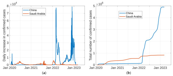
Figure 11. The curves of confirmed coronavirus cases in China and Saudi Arabia, (a) novel coronavirus daily cases, (b) total coronavirus cases.

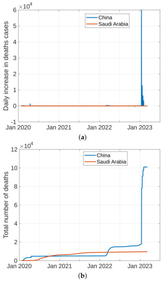
Figure 12. Curves of coronavirus death cases in China and Saudi Arabia, (a) novel coronavirus daily deaths, (b) total coronavirus deaths.

Figure 13. (a) Zoom of Figure 11a on the y-axis, (b) zoom of Figure 12a on the y-axis.

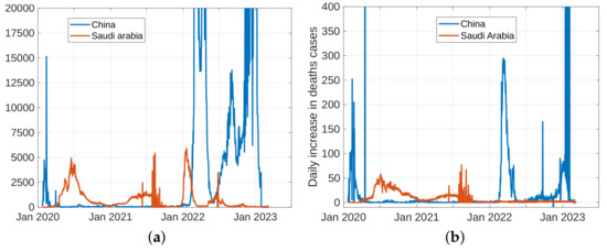
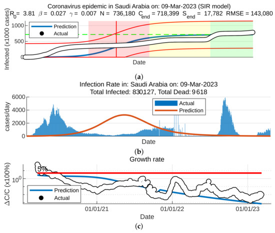
Figure 14. Curves of coronavirus cases in Saudi Arabia, (a) coronavirus epidemic in Saudi Arabia, (b) infection rate, (c) growth rate.

5.2. Results for the SIR and SEIR Systems Using the Data

Figure 15, Figure 16 and Figure 17 present the results of the discrete-time–fractional-order of the SIR and SEIR systems defined in (26) and (59) using data observed by the World Health Organization. By comparing with the results obtained from these data, it can be seen that the results given in Figure 15, Figure 16 and Figure 17, which are drawn from discrete fractional models (26) and (59), are closer to the real data than the expected numbers obtained from models (4) and (41). Furthermore, these results show that discrete fractional orders have better effects on the behaviors of continuous models.

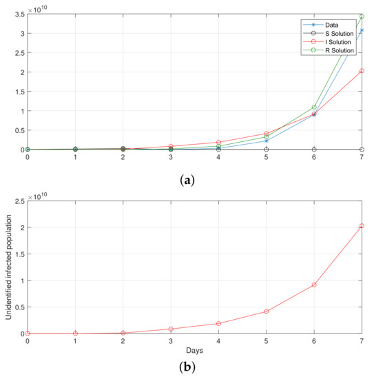
Figure 15. Computational observations from the first seven days of Saudi Arabia, with the optimization of initial values using the SIR system (26) in the discrete-time–fractional-order: (a) confirmed, recovered, and death populations; (b) unidentified infected.

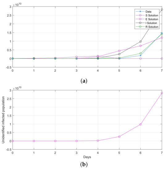
Figure 16. Computational observations from seven days in Saudi Arabia, with the optimization of initial values using the SEIR system (59) in the discrete-time–fractional-order: (a) confirmed, exposed, recovered, and death populations; (b) unidentified infected.

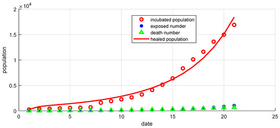
Figure 17. Curves of confirmed, exposed, recovered, and death populations using the SEIR system (59) in the discrete-time–fractional-order, using data recorded in 21 days in China.

6. Conclusions

Since the first coronavirus (COVID-19) case was discovered in China in 2019, the coronavirus pandemic has spread globally, resulting in at least 101,918,720 infections and 6,733,494 deaths worldwide as of 19 January 2023, according to statistics from Johns Hopkins University. In Saudi Arabia, the Ministry of Health noted what was happening throughout the world and imposed stricter movement restrictions; most of the population has been vaccinated. Not all populations adhere to health laws, and with a large number of people adhering to religious visits (e.g., Hajj and Umrah), the spread of the virus has been reduced. In China, due to the economic crisis and population demonstrations, the coronavirus is spreading widely. In this paper, we present a study that utilizes mathematical models of the coronavirus (i.e., discrete-time and fractional-order models), accompanied by numerical results. We presented two examples: Saudi Arabia as a country that has overcome the coronavirus, and China as a country that is still suffering from the spread of this virus, despite fighting it. As the coronavirus continues to spread in some countries, and because specific antiviral treatments and vaccines are still being developed, testing and quarantines are still being encouraged to prevent the spread of the virus. However, since the virus continues to mutate and evolve, scientific and mathematical studies must continue until it is eradicated worldwide.

References

- Liu, Y.C.; Kuo, R.L.; Shih, S.-R. COVID-19: The first documented coronavirus pandemic in history. Biomed. J. 2020, 43, 328–333. [Google Scholar] [CrossRef] [PubMed]
- Majumder, M.; Mandl, K.D. Early transmissibility assessment of a novel coronavirus in Wuhan, China. SSRN Electron. J. 2020. [Google Scholar] [CrossRef]
- Mtewa, A.G.; Amanjot, A.; Yadesa, T.M.; Ngwira, K.J. Drug repurposing for SARS-COV-2 (COVID-19) treatment. Coronavirus Drug Discov. 2022, 1, 205–226. [Google Scholar] [CrossRef]
- Yang, J.; Gong, H.; Chen, X.; Chen, Z.; Deng, X.; Qian, M.; Hou, Z.; Ajelli, M.; Viboud, C.; Yu, H. Review for health-seeking behaviors of patients with acute respiratory infections during the outbreak of novel Coronavirus Disease 2019 in Wuhan, China. Influenza Other Respir. Viruses 2020, 15, 188–194. [Google Scholar] [CrossRef] [PubMed]
- Segel, L.A.; Murray, J.D. Mathematical Biology (3rd ed), Volume I (An Introduction) and Volume II (Spatial models and biomedical applications). Math. Med. Biol. 2003, 20, 377–378. [Google Scholar] [CrossRef]
- Srinivasan, S.; Cui, H.; Gao, Z.; Liu, M.; Lu, S.; Mkandawire, W.; Narykov, O.; Sun, M.; Korkin, D. Structural genomics of SARS-COV-2 indicates evolutionary conserved functional regions of viral proteins. Viruses 2020, 12, 360. [Google Scholar] [CrossRef]
- Liu, D.X.; Liang, J.Q.; Fung, T.S. Human Coronavirus-229E, -OC43, -NL63, and -HKU1 (Coronaviridae). Encycl. Virol. 2021, 428–440. [Google Scholar] [CrossRef]
- Zhao, S.; Lin, Q.; Ran, J.; Musa, S.S.; Yang, G.; Wang, W.; Lou, Y.; Gao, D.; Yang, L.; He, D.; et al. Preliminary estimation of the basic reproduction number of novel coronavirus (2019-ncov) in China, from 2019 to 2020: A data-driven analysis in the early phase of the outbreak. Int. J. Infect. Dis. 2020, 92, 214–217. [Google Scholar] [CrossRef]
- Data Source COVID-19: Center for Systems Science and Engineering (CSSE) at Johns Hopkins University (JHU). Available online: https://coronavirus.jhu.edu/region/ (accessed on 8 April 2023).
- Msmali, A.; Mutum, Z.; Mechai, I.; Ahmadini, A. Modeling and simulation: A study on predicting the outbreak of COVID-19 in Saudi Arabia. Discret. Dyn. Nat. Soc. 2021, 2021, 5522928. [Google Scholar] [CrossRef]
- Data Source COVID-19: World Health Organization (WHO). Available online: https://covid19.who.int/data (accessed on 8 April 2023).
- Rangasamy, M.; Chesneau, C.; Martin-Barreiro, C.; Leiva, V. On a novel dynamics of SEIR epidemic models with a potential application to COVID-19. Symmetry 2022, 14, 1436. [Google Scholar] [CrossRef]
- Verma, H.; Mishra, V.N.; Mathur, P. Effectiveness of lock down to curtail the spread of Corona virus: A mathematical model. ISA Trans. 2022, 124, 124–134. [Google Scholar] [CrossRef] [PubMed]
- Saeed, T.; Djeddi, K.; Guirao, J.L.; Alsulami, H.H.; Alhodaly, M.S. A discrete dynamics approach to a tumor system. Mathematics 2022, 10, 1774. [Google Scholar] [CrossRef]
- De Natale, G.; Ricciardi, V. The COVID-19 infection in Italy: A statistical study of an abnormally severe disease. J. Clin. Med. 2020, 9, 1564. [Google Scholar] [CrossRef] [PubMed]
- Frank, T.D. COVID-19 Epidemiology and Virus Dynamics Nonlinear Physics and Mathematical Modeling; Springer: Berlin/Heidelberg, Germany, 2022. [Google Scholar]
- Kurmi, S.; Chouhan, U. A multicompartment mathematical model to study the dynamic behavior of COVID-19 using vaccination as control parameter. Nonlinear Dyn. 2022, 109, 2185–2201. [Google Scholar] [CrossRef] [PubMed]
- Mihailo, P.L.; Milan, R.R.; Tomislav, B.S. Introduction to Fractional Calculus with Brief Historical Background. 2014. Available online: https://www.researchgate.net/publication/312137269_Introduction_to_Fractional_Calculus_with_Brief_Historical_Background (accessed on 10 April 2023).
- Xu, C.; ur Rahman, M.; Baleanu, D. On fractional-order symmetric oscillator with offset-boosting control. Nonlinear Anal. Model. Control. 2022, 27, 1–15. [Google Scholar] [CrossRef]
- Khan, F.S.; Khalid, M.; Al-moneef, A.A.; Ali, A.H.; Bazighifan, O. Freelance model with Atangana–Baleanu Caputo fractional derivative. Symmetry 2022, 14, 2424. [Google Scholar] [CrossRef]
- Hamdan, N.I.; Kilicman, A. A fractional order sir epidemic model for dengue transmission. Chaos Solitons Fractals 2018, 114, 55–62. [Google Scholar] [CrossRef]
- Kamel, D. Dynamics in a Discrete—Time Three Dimensional Cancer System. Int. J. Appl. Math. 2019, 49, 1–7. [Google Scholar]
- Khennaoui, A.; Ouannas, A.; Bendoukha, S.; Grassi, G.; Lozi, R.P.; Pham, V. On fractional–order discrete–time systems: Chaos, stabilization and synchronization. Chaos Solitons Fractals 2019, 119, 150–162. [Google Scholar] [CrossRef]
- Abdulrahman, I. Simcovid: Open-source simulation programs for the COVID-19 Outbreak. Comput. Sci. 2022, 4, 20. [Google Scholar] [CrossRef]
- Chen, T.-M.; Rui, J.; Wang, Q.-P.; Zhao, Z.-Y.; Cui, J.-A.; Yin, L. A mathematical model for simulating the phase-based transmissibility of a novel coronavirus. Infect. Dis. Poverty 2020, 9, 24. [Google Scholar] [CrossRef]
- Data Source COVID-19: CSSEGISandData. (n.d.). CSSEGISANDDATA/COVID-19: Novel coronavirus (COVID-19) Cases, Provided by JHU CSSE. GitHub. Available online: https://github.com/CSSEGISandData/COVID-19 (accessed on 8 April 2023).
- Kermack, W.O.; McKendrick, A.G. A Contribution to the Mathematical Theory of Epidemics; Royal Society: London, UK, 1927; Volume 115. [Google Scholar] [CrossRef]
- Muñoz-Fernández, G.A.; Seoane, J.M.; Seoane-Sepúlveda, J.B. A sir-type model describing the successive waves of COVID-19. Chaos Solitons Fractals 2021, 144, 110682. [Google Scholar] [CrossRef] [PubMed]
- Angstmann, C.N.; Henry, B.I.; McGann, A.V. A fractional-order infectivity and Recovery Sir Model. Fractal Fract. 2017, 1, 11. [Google Scholar] [CrossRef]
- Singh, R.A.; Lal, R.; Kotti, R.R. Time-discrete SIR model for COVID-19 in Fiji. In Epidemiology and Infection; Cambridge University Press: Cambridge, MA, USA, 2022; Volume 150. [Google Scholar] [CrossRef]
- Wacker, B.; Schlüter, J. Time-continuous and time-discrete SIR models revisited: Theory and applications. Adv. Differ. Equ. 2020, 2020, 556. [Google Scholar] [CrossRef]
- Metcalfe, C. Book review: Pan J-X, Fang K-T 2002: Growth curve models and statistical diagnostics. In Statistical Methods in Medical Research; Springer: New York, NY, USA, 2007; Volume 59, pp. 341–342. ISBN 0-387-95053-2. [Google Scholar] [CrossRef]
- Su, S. Maximum Log Likelihood Estimation using EM Algorithm and Partition Maximum Log Likelihood Estimation for Mixtures of Generalized Lambda Distributions. J. Mod. Appl. Stat. Methods 2011, 10, 599–606. [Google Scholar] [CrossRef]
- Dai, Y.; Billard, L. Maximum likelihood estimation in space time bilinear models. J. Time Ser. Anal. 2003, 24, 25–44. [Google Scholar] [CrossRef]
- Salgotra, R.; Gandomi, M.; Gandomi, A.H. Time Series Analysis and Forecast of the COVID-19 Pandemic in India using Genetic Programming. Chaos Solitons Fractals 2020, 138, 109945. [Google Scholar] [CrossRef]
- Willmott, C.; Matsuura, K. Advantages of the mean absolute error (MAE) over the root mean square error (RMSE) in assessing average model performance. Clim. Res. 2005, 30, 79–82. [Google Scholar] [CrossRef]
- He, Z.Y.; Abbes, A.; Jahanshahi, H.; Alotaibi, N.D.; Wang, Y. Fractional-order discrete-time sir epidemic model with vaccination: Chaos and complexity. Mathematics 2022, 10, 165. [Google Scholar] [CrossRef]
- Gu, Y.; Khan, M.A.; Hamed, Y.S.; Felemban, B.F. A comprehensive mathematical model for SARS-COV-2 in Caputo derivative. Fractal Fract. 2021, 5, 271. [Google Scholar] [CrossRef]
- Ahmadini, A.; Msmali, A.; Mutum, Z.; Raghav, Y.S. The Mathematical Modeling Approach for the wastewater treatment process in Saudi Arabia during COVID-19 pandemic. Discret. Dyn. Nat. Soc. 2022, 2022, 1061179. [Google Scholar] [CrossRef]
- Lin, Q.; Chiu, A.P.Y.; Zhao, S.; He, D. Modeling the spread of Middle East respiratory syndrome coronavirus in Saudi Arabia. Stat. Methods Med. Res. 2018, 27, 1968–1978. [Google Scholar] [CrossRef] [PubMed]
Disclaimer/Publisher’s Note: The statements, opinions and data contained in all publications are solely those of the individual author(s) and contributor(s) and not of MDPI and/or the editor(s). MDPI and/or the editor(s) disclaim responsibility for any injury to people or property resulting from any ideas, methods, instructions or products referred to in the content. |
© 2023 by the authors. Licensee MDPI, Basel, Switzerland. This article is an open access article distributed under the terms and conditions of the Creative Commons Attribution (CC BY) license (https://creativecommons.org/licenses/by/4.0/).