Asymptotics for Time-Fractional Venttsel’ Problems in Fractal Domains

Abstract

In this study, we consider fractional-in-time Venttsel’ problems in fractal domains of the Koch type. Well-posedness and regularity results are given. In view of numerical approximation, we consider the associated approximating pre-fractal problems. Our main result is the convergence of the solutions of such problems towards the solution of the fractional-in-time Venttsel’ problem in the corresponding fractal domain. This is achieved via the convergence (in the Mosco–Kuwae–Shioya sense) of the approximating energy forms in varying Hilbert spaces.

1. Introduction

The aim of this paper was to study the asymptotic behavior of the solution of time-fractional Venttsel’ problems $\left({\overline{P}}_h\right)$ in Koch-type pre-fractal domains ${\mathrm{\Omega }}_h$, and to prove that the limit is the solution of the corresponding problem $\left(\overline{P}\right)$ in the Koch domain $\mathrm{\Omega }$. Beyond the interest in itself, this result is a preliminary step towards the numerical approximation of problem $\left(\overline{P}\right)$, following the approach of [1].

Fractal geometries are good models for irregular media, and many diffusion phenomena take place across irregular layers. This motivates the study of fractional heat diffusion across irregular boundaries.

From the mathematical point of view, the problem can be viewed as the coupling of an evolution equation in the bulk and an evolution equation on the boundary. These problems are also known as boundary value problems (BVPs) with dynamical boundary conditions. In the present setting, the resulting boundary condition is of the second order, which is, in some sense, unusual for BVPs involving second order operators.

We formally state the model problem $\left(\overline{P}\right)$ as:

$$\left(\overline{P}\right)\left\{\begin{array}{cc}{\partial }_t^{\alpha }u(t,P)-\Delta u(t,P)=f(t,P)\hfill & \mathrm{in}(0,T)\times \mathrm{\Omega },\hfill \\ {\partial }_t^{\alpha }u(t,P)-{\Delta }_{K}u(t,P)+b\left(P\right)u(t,P)+\frac{\partial u(t,P)}{\partial n}=f(t,P)\hfill & \mathrm{in}(0,T)\times K,\hfill \\ u(0,P)=\phi \left(P\right)\hfill & \mathrm{in}\overline{\mathrm{\Omega }},\hfill \end{array}\right.$$

where $\mathrm{\Omega }\subset {\mathbb{R}}^2$ is the two-dimensional open bounded domain with boundary $K=\partial \mathrm{\Omega }$, the Koch snowflake (see Section 2.1), $0<\alpha \le 1$, ${\partial }_t^{\alpha }$ is the fractional Caputo time derivative (see Section 2.5 for the definition), ${\Delta }_K$ is the Laplace operator defined on the fractal K (see (8) in Section 3.1), b is a continuous strictly positive function on $\overline{\mathrm{\Omega }}$, $\frac{\partial u}{\partial n}$ denotes the normal derivative across $K,$f and $\phi$ are given data in suitable functional spaces (see Section 4).

For $h\in \mathbb{N}$, we denote by ${\mathrm{\Omega }}_h\subset {\mathbb{R}}^2$ the pre-fractal domain with boundary $\partial {\mathrm{\Omega }}_h=K_h$, where $K_h$ is the polygonal curve approximating K at the h-th step (see Section 2.1).

We consider the problems $\left({\overline{P}}_h\right)$ defined on ${\mathrm{\Omega }}_h$. For every $h\in \mathbb{N}$, we formally present problem $\left({\overline{P}}_h\right)$ as:

$$\left({\overline{P}}_h\right)\left\{\begin{array}{cc}{\partial }_t^{\alpha }{u}_h(t,P)-\Delta u_h(t,P)=f_h(t,P)\hfill & \mathrm{in}(0,T)\times {\mathrm{\Omega }}_h,\hfill \\ {\delta }_h{\partial }_t^{\alpha }{u}_h(t,P)-{\Delta }_{K_h}{u}_h(t,P)+{\delta }_{h}b\left(P\right)u_h(t,P)+\frac{\partial u_h(t,P)}{\partial n_h}={\delta }_h{f}_h(t,P)\hfill & \mathrm{in}(0,T)\times K_h,\hfill \\ u_h(0,P)={\phi }_h\left(P\right)\hfill & \mathrm{in}{\overline{\mathrm{\Omega }}}_h,\hfill \end{array}\right.$$

where ${\Delta }_{K_h}$ is the piecewise tangential Laplacian defined on $K_h$ (see Section 3.2), $\frac{\partial u_h}{\partial n_h}$ is the normal derivative across $K_h$ and $f_h(t,P)$ and ${\phi }_h\left(P\right)$ are given data in suitable functional spaces. The positive constant ${\delta }_h$ has a key role in the asymptotic behavior as $h\to +\infty$ (see Section 5). The choice of this constant allows us to overcome the difficulties arising from the jump of dimension in the asymptotic analysis from the pre-fractal case to the fractal one.

We remark that Venttsel’ problems in fractal domains, and their approximations, were first studied in [2], see also [3,4,5]. These problems were later generalized to the case of quasi-linear and/or fractional-in-space operators, as, for example, in [6,7].

The literature on Venttsel’ problems in smooth domains is huge, starting from the pioneering work of Venttsel’ in 1959 [8], wherein he introduced a new class of boundary conditions for elliptic operators given by second order integro-differential equations (see also [9,10,11,12,13]). We refer the reader to the introduction of [2] for the physical motivations, and also [14].

As to the literature on time-fractional problems, the existing literature is wide. Among others, we refer to [15,16,17,18,19,20], and the references therein, and to [21] for time-fractional Venttsel’ problems in Lipschitz domains. For time-fractional equations in fractal domains, we refer to, for example, [22,23].

Our goal is to prove well-posedness results for problems $\left(\overline{P}\right)$ and $\left({\overline{P}}_h\right)$ and to prove that the “fractal” solution of problem $\left(\overline{P}\right)$ can be approximated by the sequence $\left\{u_h\right\}$ of the “smoother” solutions of problems $\left({\overline{P}}_h\right)$.

More precisely, in Section 4.1 we introduce abstract Cauchy problems $\left(P\right)$ and $\left(P_h\right)$ and we prove that problem $\left(\overline{P}\right)$ is the “strong formulation” of problem $\left(P\right)$ (see Theorem 3) and that, for every $h\in \mathbb{N}$, problem $\left({\overline{P}}_h\right)$ is the “strong formulation” of problem $\left(P_h\right)$ (see Theorem 4). Existence and uniqueness results of the “strong solution” are obtained by the well-posedness results for fractional-in-time Cauchy problems [21].

We emphasize that the natural functional framework for studying problems $\left(P_h\right)$ is that of the varying spaces $L^2({\overline{\mathrm{\Omega }}}_h,m_h)$ (see Section 5.1).

The asymptotic analysis of the solutions of problems $\left({\overline{P}}_h\right)$ is performed by using the Mosco–Kuwae–Shioya (M-K-S) convergence. In [2], it was proved that the energy forms $E^{\left(h\right)}$, associated to problems $\left({\overline{P}}_h\right)$, converge in the M–K–S sense to the fractal energy form E, associated to problem $\left(\overline{P}\right)$. This implies the convergence of associated semigroups and resolvents and it turns out to be crucial for the proof of Theorem 6.

The plan of the paper is the following.

In Section 2, we recall the geometry, the functional setting, and the definition of convergence of varying Hilbert spaces, as well as the definition of the fractional Caputo time derivative.

In Section 3, we introduce the energy forms E and $E^{\left(h\right)}$, see (11) and (17), respectively, and the associated resolvents and semigroups.

In Section 4, we study the existence and uniqueness of the solutions of the evolution problems $\left(P\right)$ and $\left(P_h\right)$. Moreover, we give the strong formulations of problems $\left(P\right)$ and $\left(P_h\right)$.

In Section 5, we state the convergence of the energy forms and of the Hilbert spaces and in Theorem 6 we prove the convergence of the pre-fractal solutions to the fractal solution in a suitable weak sense.

2. Preliminaries

2.1. Geometry

In this paper, we denote points in ${\mathbb{R}}^2$ by $P=(x_1,x_2)$, the Euclidean distance by $|P-P_0|$ and the Euclidean ball by $B(P_0,r)=\{P\in {\mathbb{R}}^2:|P-P_0|<r\}$ for $P_0\in {\mathbb{R}}^2$ and $r>0$. The Koch snowflake K [24] is the union of three com-planar Koch curves $K_1$, $K_2$ and $K_3$, see Figure 1.

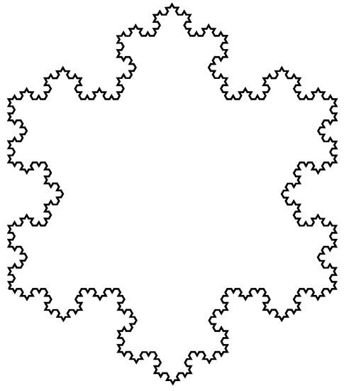
Figure 1. The Koch snowflake K.

The Hausdorff dimension of the Koch snowflake is $d_f=\frac{ln4}{ln3}$.

The natural finite Borel measure $\mu$, supported on K, is defined as

$$\mu :={\mu }_1+{\mu }_2+{\mu }_3,$$

(1)

where ${\mu }_i$ denotes the normalized $d_f$-dimensional Hausdorff measure, restricted to $K_i$, $i=1,2,3$.

We denote by

$${\displaystyle K_{h+1}=\bigcup _{i=1}^3{K}_i^{(h+1)}}$$

(2)

the closed polygonal curve approximating K at the $(h+1)$-th step. We denote by $K_i^{(h+1)}$ the pre-fractal (polygonal) curve approximating $K_i$.

The measure $\mu$ enjoys the following property: there exist two positive constants $c_1$, $c_2$ such that

$$c_1{r}^{d_f}\le \mu (B(P,r)\cap K)\le c_2{r}^{d_f}\forall P\in K.$$

(3)

Since $\mu$ is supported on K, in (3) we replace $\mu \left(B\right(P,r)\cap K)$ with $\mu \left(B\right(P,r\left)\right)$.

Let $\mathrm{\Omega }$ denote the two-dimensional open bounded domain with boundary K and, for every $h\in \mathbb{N}$, let ${\mathrm{\Omega }}_h$ be the pre-fractal polygonal domains approximating $\mathrm{\Omega }$ at the n-th step, and let $K_h=\partial {\mathrm{\Omega }}_h$ be the pre-fractal curves. We denote by M and by $\stackrel{\circ }{M}$ any segment of $K_h$ and the related open segment, respectively. We note that the sequence ${\left\{{\mathrm{\Omega }}_h\right\}}_{h\in \mathbb{N}}$ is an invading sequence of sets exhausting $\mathrm{\Omega }$.

2.2. Sobolev Spaces

Throughout the paper, C denotes possibly different positive constants. The dependence of such constants on some parameters is given in parentheses.

Let $\mathcal{G}$ (resp. $\mathcal{S}$) be an open (resp. a closed) set of ${\mathbb{R}}^N$. For $p\ge 1$, we denote the Lebesgue space with respect to the Lebesgue measure $\mathrm{d}{\mathcal{L}}_N$ by $L^p\left(\mathcal{G}\right)$ and the Lebesgue space on $\partial \mathcal{G}$ with respect to an invariant Hausdorff measure $\mu$ supported on $\partial \mathcal{G}$ by $L^p(\partial \mathcal{G},\mu ).$ For $s\in {\mathbb{R}}^{+},$ we denote the usual (possibly fractional) Sobolev spaces by $H^s\left(\mathcal{G}\right)$ [25]. We denote the space of infinitely differentiable functions with compact support on $\mathcal{G}$ by $\mathcal{D}\left(\mathcal{G}\right)$ and the space of continuous functions on $\mathcal{S}$ by $C\left(\mathcal{S}\right).$

In the following, we make use of trace spaces on boundaries of polygonal domains of ${\mathbb{R}}^2$. For more details, we refer the reader to [26].

By $H^1\left(K_h\right)$ we denote the set

$$\{v\in C\left(K_h\right):u{|}_{\stackrel{\circ }{M}}\in H^1(\stackrel{\circ }{M})\},$$

with the norm

$${\parallel u\parallel }_{H^1\left(K_h\right)}^2={\parallel u\parallel }_{L^2\left(K_h\right)}^2+{\parallel \nabla u\parallel }_{L^2\left(K_h\right)}^2.$$

By $H^s\left(K_h\right)$, for $0<s\le 1$, we denote the Sobolev space on $K_h$, defined by local Lipschitz charts as in [25]. We point out that for $s=1$ the two definitions coincide with equivalent norms.

By $\left|A\right|$ we denote the Lebesgue measure of a measurable subset $A\subset {\mathbb{R}}^N$. For f in $H^s\left(\mathcal{G}\right)$, the trace operator ${\gamma }_0$ is defined as

$${\gamma }_{0}f\left(P\right):=\underset{r\to 0}{lim}\frac{1}{\left|B\right(P,r)\cap \mathcal{G}|}{\int }_{B(P,r)\cap \mathcal{G}}f\left(Q\right)\mathrm{d}{\mathcal{L}}_N\left(Q\right)$$

(4)

at every point $P\in \overline{\mathcal{G}}$ where the limit exists. The limit (4) exists at quasi every $P\in \overline{\mathcal{G}}$ with respect to the $(s,2)$-capacity (see [27], Definition 2.2.4 and Theorem 6.2.1 page 159). In the following, we sometimes omit the trace symbol, leaving the interpretation to the reader.

We now recall the results of Theorem 2.24 in [26], referring to [28] for a more general discussion.

Proposition 1. 

Let ${\mathrm{\Omega }}_h$ and $K_h$ be as above and let $\frac{1}{2}<s<\frac{3}{2}$. Then $H^{s-\frac{1}{2}}\left(K_h\right)$ is the trace space to $K_h$ of $H^s\left({\mathrm{\Omega }}_h\right)$ in the following sense:

(i) 

${\gamma }_0$ is a linear and continuous operator from $H^s\left({\mathrm{\Omega }}_h\right)$ to $H^{s-\frac{1}{2}}\left(K_h\right)$;

(ii) 

there exists a linear and continuous operator Ext from $H^{s-\frac{1}{2}}\left(K_h\right)$ to $H^s\left({\mathrm{\Omega }}_h\right)$ such that ${\gamma }_0\circ \mathrm{Ext}$ is the identity operator in $H^{s-\frac{1}{2}}\left(K_h\right)$.

In the sequel we denote by the symbol ${f|}_{K_h}$ the trace ${\gamma }_{0}f$ to $K_h$.

2.3. Besov Spaces

We start by giving the definition of d-set.

Definition 1. 

Let $\mathcal{S}\subset {\mathbb{R}}^N$ be closed and non-empty. $\mathcal{S}$ is a d-set, for $0<d\le N$, if there exists a Borel measure $\tilde{\mu }$, with $supp\tilde{\mu }=\mathcal{S}$ and two constants $c_1=c_1\left(\mathcal{S}\right)>0$ and $c_2=c_2\left(\mathcal{S}\right)>0$, such that

$$c_1{r}^d\le \tilde{\mu }\left(B(P,r)\right)\le c_2{r}^d\forall P\in \mathcal{S},0<r\le 1.$$

(5)

Such a measure $\tilde{\mu }$ is called a d-measure on $\mathcal{S}$.

The following result follows from [24].

Proposition 2. 

Let $d=d_f$. Then the measure μ defined in (3) is a d-measure, and, hence, the Koch snowflake K is a d-set.

We recall the definition of Besov spaces specialized to our case. For generalities on Besov spaces, we refer the reader to [29,30].

Definition 2. 

Let $\mathcal{S}$ be a d-set in ${\mathbb{R}}^N$ and $0<\gamma <1$. We say that $f\in B_{\gamma }^{2,2}\left(\mathcal{S}\right)$ if

$${\parallel f\parallel }_{B_{\gamma }^{2,2}\left(\mathcal{S}\right)}^2:={\parallel f\parallel }_{L^2(\mathcal{S},\tilde{\mu })}^2+{\displaystyle {\int \int }_{|P-P^{\prime }|<3^{-n}}}\frac{|f\left(P\right)-f\left(P^{\prime }\right){|}^2}{|P-P^{\prime }{|}^{d+2\gamma }}\mathrm{d}\tilde{\mu }\left(P\right)\mathrm{d}\tilde{\mu }\left(P^{\prime }\right)<\infty .$$

We now state the trace theorem specialized to our case.

Proposition 3. 

$B_{\frac{d_f}{2}}^{2,2}\left(K\right)$ is the trace space to K of $H^1\left(\mathrm{\Omega }\right)$ in the following sense:

(i) 

${\gamma }_0$ is a linear and continuous operator from $H^1\left(\mathrm{\Omega }\right)$ to $B_{\frac{d_f}{2}}^{2,2}\left(K\right)$;

(ii) 

there exists a linear and continuous operator Ext from $B_{\frac{d_f}{2}}^{2,2}\left(K\right)$ to $H^1\left(\mathrm{\Omega }\right)$ such that ${\gamma }_0\circ \mathrm{Ext}$ is the identity operator in $B_{\frac{d_f}{2}}^{2,2}\left(K\right)$.

For the proof, we refer to Theorem 1 of Chapter VII in [29], and see also [30]. The symbol ${f|}_K$ denotes the trace ${\gamma }_{0}f$ to K.

As to the dual of Besov spaces on K, we refer to [31], where it is shown that they coincide with a subspace of Schwartz distributions ${\mathcal{D}}^{\prime }\left({\mathbb{R}}^2\right)$, supported on K. For a complete discussion and description of duals of Besov spaces on d-sets, see [31].

2.4. Convergence of Hilbert Spaces

In this subsection, we recall the definition of convergence of varying real and separable Hilbert spaces (for definitions and proofs, see [32,33]).

Definition 3. 

A sequence of Hilbert spaces ${\left\{H_h\right\}}_{h\in \mathbb{N}}$ converges to a Hilbert space H if there exists a dense subspace $C\subset H$ and a sequence ${\left\{Z_h\right\}}_{h\in \mathbb{N}}$ of linear operators $Z_h:C\subset H\to H_h$, such that

$$\underset{h\to \infty }{lim}{∥Z_{h}u∥}_{H_h}={∥u∥}_{H}foranyu\in C.$$

In the following, we assume that ${\left\{H_h\right\}}_{h\in \mathbb{N}}$, H and ${\left\{Z_h\right\}}_{h\in \mathbb{N}}$ are as in Definition 3. Let $\mathcal{H}=\left\{{\cup }_h{H}_h\right\}\cup H.$ We recall the definition of strong convergence in $\mathcal{H}$.

Definition 4. 

(Strong convergence in $\mathcal{H}$). A sequence of vectors ${\left\{u_h\right\}}_{h\in \mathbb{N}}$ strongly converges to u in $\mathcal{H}$ if $u_h\in H_h$, $u\in H$ and there exists a sequence ${\left\{{\tilde{u}}_m\right\}}_{m\in \mathbb{N}}\in C$ tending to u in H, such that

$$\underset{m\to \infty }{lim}\underset{h\to \infty }{\overline{lim}}{∥Z_h{\tilde{u}}_m-u_h∥}_{H_h}=0.$$

We recall the definition of strong convergence in $\mathcal{H}$.

Definition 5. 

(Weak convergence in $\mathcal{H}$) A sequence of vectors ${\left\{u_h\right\}}_{h\in \mathbb{N}}$ weakly converges to u in $\mathcal{H}$ if $u_h\in H_h$, $u\in H$ and

$${(u_h,v_h)}_{H_h}\to {(u,v)}_H$$

for every sequence ${\left\{v_h\right\}}_{h\in \mathbb{N}}$ strongly tending to v in $\mathcal{H}$.

We point out that the strong convergence implies the weak convergence [33].

Lemma 1. 

Let ${\left\{u_h\right\}}_{h\in \mathbb{N}}$ be a sequence weakly converging to u in $\mathcal{H}$. Then

$$\underset{h}{sup}{∥u_h∥}_{H_h}<\infty ,{∥u∥}_H\le \underset{h\to \infty }{\underline{lim}}{∥u_h∥}_{H_h}.$$

Moreover, $u_h\to u$ strongly if, and only if, ${\parallel u\parallel }_H=\underset{h\to \infty }{lim}{\parallel u_h\parallel }_{H_h}$.

We recall some useful properties of the strong convergence of a sequence of vectors ${\left\{u_h\right\}}_{h\in \mathbb{N}}$ in $\mathcal{H}$.

Lemma 2. 

Let $u\in H$ and let ${\left\{u_h\right\}}_{h\in \mathbb{N}}$ be a sequence of vectors $u_h\in H_h$. Then, ${\left\{u_h\right\}}_{h\in \mathbb{N}}$ strongly converges to u in $\mathcal{H}$ if, and only if,

$${(u_h,v_h)}_{H_h}\to {(u,v)}_H$$

for every sequence ${\left\{v_h\right\}}_{h\in \mathbb{N}}$ with $v_h\in H_h$ weakly converging to a vector v in $\mathcal{H}$.

Lemma 3. 

A sequence of vectors ${\left\{u_h\right\}}_{h\in \mathbb{N}}$ with $u_h\in H_h$ strongly converges to a vector u in $\mathcal{H}$ if, and only if,

$$\begin{array}{ccc}\hfill {∥u_h∥}_{H_h}& \to & {∥u∥}_{H}and\hfill \\ \hfill {(u_h,Z_h\left(\phi \right))}_{H_h}& \to & {(u,\phi )}_{H}forevery\phi \in C.\hfill \end{array}$$

Lemma 4. 

Let ${\left\{u_h\right\}}_{h\in \mathbb{N}}$ be a sequence with $u_h\in H_h$. If $\parallel u_h{\parallel }_{H_h}$ is uniformly bounded, then there exists a subsequence of ${\left\{u_h\right\}}_{h\in \mathbb{N}}$, which weakly converges in $\mathcal{H}$.

Lemma 5. 

For every $u\in H$ there exists a sequence ${\left\{u_h\right\}}_{h\in \mathbb{N}}$, with $u_h\in H_h$, strongly converging to u in $\mathcal{H}$.

We denote by $\mathfrak{L}\left(X\right)$ the space of linear and continuous operators on a Hilbert space X.

We now recall the notion of the strong convergence of operators.

Definition 6. 

A sequence of bounded operators ${\left\{B_h\right\}}_{h\in \mathbb{N}}$, with $B_h\in \mathfrak{L}\left(H_h\right)$, strongly converges to an operator $B\in \mathfrak{L}\left(H\right)$ if for every sequence of vectors ${\left\{u_h\right\}}_{h\in \mathbb{N}}$ with $u_h\in H_h$ strongly converging to a vector u in $\mathcal{H}$, the sequence $\left\{B_h{u}_h\right\}$ strongly converges to $Bu$ in $\mathcal{H}$.

2.5. Fractional-in-Time Derivatives

We recall the notion of fractional-in-time derivatives in the sense of Riemann–Liouville and Caputo by using the notations of the monograph [21].

Let $\alpha \in (0,1)$. We define

$$g_{\alpha }\left(t\right)=\left\{\begin{array}{cc}{\displaystyle \frac{t^{\alpha -1}}{\mathrm{\Gamma }\left(\alpha \right)}}\hfill & \mathrm{if}t>0,\hfill \\ 0\hfill & \mathrm{if}t\le 0,\hfill \end{array}\right.$$

where $\mathrm{\Gamma }$ is the usual Gamma function.

Definition 7. 

Let Y be a Banach space, $T>0$ and let $f\in C\left(\right[0,T];Y)$ be such that $g_{1-\alpha }\ast f\in W^{1,1}((0,T);Y)$.

(i) 

The Riemann–Liouville fractional derivative of order $\alpha \in (0,1)$ is defined as follows:

$$D_t^{\alpha }f\left(t\right):=\frac{\mathrm{d}}{\mathrm{d}t}(g_{1-\alpha }\ast f)\left(t\right)=\frac{\mathrm{d}}{\mathrm{d}t}{\int }_0^t{g}_{1-\alpha }(t-\tau )f\left(\tau \right)\mathrm{d}\tau ,$$

for a.e. $t\in (0,T]$.

(ii) 

The Caputo-type fractional derivative of order $\alpha \in (0,1)$ is defined as follows:

$${\partial }_t^{\alpha }f\left(t\right):=D_t^{\alpha }(f\left(t\right)-f\left(0\right)),$$

for a.e. $t\in (0,T]$.

We stress the fact that Definition 7-$\left(ii\right)$ gives a weaker definition of the (Caputo) fractional derivative with respect to the original one (see [34]), since f is not assumed to be differentiable. Moreover, it holds that ${\partial }_t^{\alpha }\left(c\right)=0$ for every constant $c\in \mathbb{R}$.

We refer to [17] for further details on fractional derivatives.

In the next sections we consider problems of the following type:

$$\left(\tilde{P}\right)\left\{\begin{array}{cc}{\partial }_t^{\alpha }u-Au=f\hfill & \mathrm{a}.\mathrm{e}.\mathrm{in}\mathrm{\Omega },\mathrm{for}\mathrm{all}t\in (0,T),\hfill \\ u\left(0\right)=\phi \hfill & \mathrm{in}\mathrm{\Omega }.\hfill \end{array}\right.$$

Here, A is a closed linear operator with domain $D\left(A\right)$ in a Banach space Y, $f:[0,\infty )\to Y$ and $\phi \in Y$ are given.

According to ([21], Definition 2.1.4), we give the following notion of strong solution for problem $\left(\tilde{P}\right)$.

Definition 8. 

Let $0<T_1\le T_2<T$. We say that u is a strong solution of $\left(\tilde{P}\right)$ on the interval $I=[0,T]$ if the following conditions are satisfied.

(i) 

(The case $\alpha =1$) The function $u\in C\left(\right[0,T);Y)$ is such that $u\left(0\right)=\phi$, $u\left(t\right)\in D\left(A\right)$ for all $t\in [T_1,T_2]\subset I$, and ${\partial }_{t}u\in C([T_1,T_2];Y)$. Moreover, the equation ${\partial }_{t}u\left(t\right)=Au\left(t\right)+f\left(t\right)$ is satisfied on $[T_1,T_2]\subset I$.

(ii) 

(The case $\alpha \in (0,1)$) The function $u\in C\left(\right[0,T);Y)$ is such that $u\left(0\right)=\phi$, $u\left(t\right)\in D\left(A\right)$ for $t\in [T_1,T_2]$, and ${\partial }_t^{\alpha }u\in C([T_1,T_2];Y)$. Moreover, the equation ${\partial }_t^{\alpha }u\left(t\right)=Au\left(t\right)+f\left(t\right)$ is satisfied on $[T_1,T_2]\subset I$.

3. The Energy Forms

We now introduce energy forms associated to the formal problems $\left(\overline{P}\right)$ and $\left({\overline{P}}_h\right)$, respectively. From now on, let $\mathrm{\Omega }$, K, ${\mathrm{\Omega }}_h$ and $K_h$ be as defined in Section 2.1 and let b denote a strictly positive continuous function in $\overline{\mathrm{\Omega }}$.

3.1. The Fractal Energy Form

As in ([2], Section 3.1), we introduce a Lagrangian measure ${\mathcal{L}}_K$ on K and the corresponding energy form $E_K$ as

$$E_K(u,v)={\int }_K\mathrm{d}{\mathcal{L}}_K(u,v)$$

(6)

with domain $D\left(K\right)$. This space is a Hilbert space with norm

$${\parallel u\parallel }_{D\left(K\right)}={\left({\parallel u\parallel }_{L^2\left(K\right)}^2+E_K(u,u)\right)}^{\frac{1}{2}}$$

(7)

and has been characterized in terms of the domains of the energy forms on $K_i$.

In the following we omit the subscript K, the Lagrangian measure is simply denoted by $\mathcal{L}(u,v)$ and we set $\mathcal{L}\left[u\right]=\mathcal{L}(u,u)$.

As in Proposition 3.1 of [2], the following result holds.

Proposition 4. 

In the previous notations and assumptions, the form $E_K$ with domain $D\left(K\right)$ is a regular Dirichlet form in $L^2\left(K\right)$ and the space $D\left(K\right)$ is a Hilbert space under the intrinsic norm (7).

For the definition and properties of Dirichlet forms, see [35].

We now introduce the Laplace operator on K. Since $(E_K,D\left(K\right))$ is a densely defined regular Dirichlet form on $L^2\left(K\right)$, from ([36], Chapter 6, Theorem 2.1) there exists a unique self-adjoint, non-positive operator ${\Delta }_K$ on $L^2\left(K\right)$, with domain $D\left({\Delta }_K\right)\subseteq D\left(K\right)$ dense in $L^2\left(K\right)$, such that

$$E_K(u,v)=-{\int }_K\left({\Delta }_{K}u\right)v\mathrm{d}\mu ,u\in D\left({\Delta }_K\right),v\in D\left(K\right).$$

(8)

We denote by ${\left(D\left(K\right)\right)}^{\prime }$ the dual space of $D\left(K\right)$. We now introduce the Laplace operator on K as a variational operator from $D\left(K\right)$ to ${\left(D\left(K\right)\right)}^{\prime }$ by

$$E_K(u,w)=-{⟨{\Delta }_{K}z,w⟩}_{{\left(D\left(K\right)\right)}^{\prime },D\left(K\right)},z\in D\left(K\right),w\in D\left(K\right),$$

(9)

where ${⟨·,·⟩}_{{\left(D\left(K\right)\right)}^{\prime },D\left(K\right)}$ denotes the duality pairing between ${\left(D\left(K\right)\right)}^{\prime }$ and $D\left(K\right)$. In the following ${\Delta }_K$ denote the Laplace operator both as the self-adjoint operator (see (8)) and as the variational operator (see (9)), leaving the interpretation to the context.

We now define the space of functions

$$V(\mathrm{\Omega },K)=\left\{u\in H^1{\left(\mathrm{\Omega }\right):u|}_K\in D\left(K\right)\right\}.$$

(10)

We remark that the space $V(\mathrm{\Omega },K)$ is non-trivial.

We introduce the energy form

$$E\left[u\right]={\int }_{\mathrm{\Omega }}{|\nabla u|}^2\mathrm{d}{\mathcal{L}}_2+E_K\left[u{|}_K\right]+{\int }_K{b\left|u\right|}_K{|}^2\mathrm{d}\mu$$

(11)

defined on the domain $V(\mathrm{\Omega },K)$. In the following, we denote by $L^2(\overline{\mathrm{\Omega }},m)$ the Lebesgue space with respect to the measure m with

$$\mathrm{d}m=\mathrm{d}{\mathcal{L}}_2+\mathrm{d}\mu .$$

(12)

By $E(u,v)$, for $u,v\in V(\mathrm{\Omega },K)$, we denote the corresponding bilinear form

$$E(u,v)={\int }_{\mathrm{\Omega }}\nabla u\nabla v\mathrm{d}{\mathcal{L}}_2+E_K{\left(u\right|}_K,v{|}_K)+{\int }_{K}bu{{|}_{K}v|}_K\mathrm{d}\mu .$$

(13)

Proposition 5. 

The form E, defined in (11), is a Dirichlet form in $L^2(\overline{\mathrm{\Omega }},m)$ and the space $V(\mathrm{\Omega },K)$ is a Hilbert space equipped with the scalar product

$${(u,v)}_{V(\mathrm{\Omega },K)}={(u,v)}_{H^1\left(\mathrm{\Omega }\right)}+E_K(u,v)+{(u,v)}_{L^2\left(K\right)}.$$

(14)

We denote, by ${\parallel u\parallel }_{V(\mathrm{\Omega },K)}$, the norm in $V(\mathrm{\Omega },K)$ associated with (14), i.e.,

$${\parallel u\parallel }_{V(\mathrm{\Omega },K)}={\left({\parallel u\parallel }_{H^1\left(\mathrm{\Omega }\right)}^2+{\parallel u\parallel }_{D\left(K\right)}^2\right)}^{\frac{1}{2}}.$$

(15)

3.2. The Pre-Fractal Energy Forms

For each $h\in \mathbb{N}$, we construct the energy forms $E_{K_h}$ on the pre-fractal boundaries $K_h$. By ℓ we denote the natural arc-length coordinate on each segment of the polygonal curve $K_h$ and we introduce the coordinates $x_1=x_1(\ell )$, $x_2=x_2(\ell )$, on every segment $M_h^{\left(j\right)}$ of $K_h$, $j=1,\cdots ,4^h$. By $\mathrm{d}\ell$ we denote the one-dimensional measure given by the arc-length ℓ.

Let $u\in H^1\left(K_h\right)$, where we recall that $H^1\left(K_h\right)$ is the Sobolev space on the piecewise affine set $K_h$ (see Section 2.2). We define $E_{K_h}\left[u\right]$ by setting

$$E_{K_h}\left[u\right]=\sum _{j=1}^{4^h}{\int }_{M_h^{\left(j\right)}}{\sigma }_h|{\nabla }_{\ell }u{{|}_{K_h}|}^2\mathrm{d}\ell ,$$

(16)

where ${\sigma }_h$ is a positive constant and ${\nabla }_{\ell }$ denotes the tangential derivative along the pre-fractal $K_h$. We denote the corresponding bilinear form by $E_{K_h}(u,v)$.

Let $V({\mathrm{\Omega }}_h,K_h)$ be the space of restrictions to ${\mathrm{\Omega }}_h$ of functions u defined on $\mathrm{\Omega }$ for which the following norm is finite:

$${\parallel u\parallel }_{V({\mathrm{\Omega }}_h,K_h)}^2={\parallel u\parallel }_{H^1\left({\mathrm{\Omega }}_h\right)}^2+{\parallel u\parallel }_{H^1\left(K_n\right)}^2.$$

We point out that this space is not trivial as it contains $C^{\infty }\left(\mathrm{\Omega }\right)\cap H^1\left(\mathrm{\Omega }\right)$ (see [37]).

We now consider the following energy form defined on $V({\mathrm{\Omega }}_h,K_h)$:

$$E^{\left(h\right)}\left[u\right]={\int }_{{\mathrm{\Omega }}_h}{|\nabla u|}^2\mathrm{d}{\mathcal{L}}_2+E_{K_h}\left[u{|}_{K_h}\right]+{\delta }_h{\int }_{K_h}{b\left|u\right|}_{K_h}{|}^2\mathrm{d}\ell ,$$

(17)

where ${\delta }_h$ is a positive constant.

By $E^{\left(h\right)}(u,v)$ we denote the corresponding bilinear form defined on $V({\mathrm{\Omega }}_h,K_h)\times V({\mathrm{\Omega }}_h,K_h)$:

$$E^{\left(h\right)}(u,v)={\int }_{{\mathrm{\Omega }}_h}\nabla u\nabla v\mathrm{d}{\mathcal{L}}_2+E_{K_h}{\left(u\right|}_{K_h}{,v|}_{K_h})+{\delta }_h{\int }_{K_h}bu{{|}_{K_h}v|}_{K_h}\mathrm{d}\ell .$$

(18)

In the following, we consider also the space $L^2({\overline{\mathrm{\Omega }}}_h,m_h)$, where $m_h$ is the measure given by

$$\mathrm{d}{m}_h=\mathrm{d}{\mathcal{L}}_2+{\chi }_{K_h}{\delta }_h\mathrm{d}\ell .$$

(19)

Proposition 6. 

The form $E^{\left(h\right)}$ with domain $V({\mathrm{\Omega }}_h,K_h)$, defined in (17), is a Dirichlet form in $L^2({\overline{\mathrm{\Omega }}}_h,m_h)$ and the space $V({\mathrm{\Omega }}_h,K_h)$ is a Hilbert space equipped with the norm

$${\parallel u\parallel }_{V({\mathrm{\Omega }}_h,K_h)}={\left({\int }_{{\mathrm{\Omega }}_h}{|\nabla u|}^2\mathrm{d}{\mathcal{L}}_2+E_{K_h}\left[u{|}_{K_h}\right]+{\parallel u\parallel }_{L^2({\overline{\mathrm{\Omega }}}_h,m_h)}^2\right)}^{\frac{1}{2}}.$$

(20)

3.3. Resolvents and Associated Semigroups

Since $(E,V(\mathrm{\Omega },K\left)\right)$ is a densely defined closed bilinear form on $L^2(\overline{\mathrm{\Omega }},m)$, from ([36], Chapter 6, Theorem 2.1) there exists a unique self-adjoint non-positive operator A on $L^2(\overline{\mathrm{\Omega }},m)$, with domain $D\left(A\right)\subseteq V(\mathrm{\Omega },K)$ dense in $L^2(\overline{\mathrm{\Omega }},m)$, such that

$$E(u,v)={\left(-Au,v\right)}_{L^2(\overline{\mathrm{\Omega }},m)},u\in D\left(A\right),v\in V(\mathrm{\Omega },K).$$

(21)

Moreover, in Theorem 13.1 of [35] it is proved that, to each closed symmetric form E, a family of linear operators $\{G_{\lambda },\lambda >0\}$ can be associated, with the property

$$E(G_{\lambda }u,v)+\lambda {(G_{\lambda }u,v)}_{L^2(\overline{\mathrm{\Omega }},m)}={(u,v)}_{L^2(\overline{\mathrm{\Omega }},m)},u\in L^2(\overline{\mathrm{\Omega }},m),v\in V(\mathrm{\Omega },K).$$

This family $\{G_{\lambda },\lambda >0\}$ is a strongly continuous resolvent with generator A, which also generates a strongly continuous semigroup ${\left\{T\left(t\right)\right\}}_{t\ge 0}$.

Proceeding as above, we denote by $\{G_{\lambda }^h,\lambda >0\}$, $A_h$ and ${\left\{T_h\left(t\right)\right\}}_{t\ge 0}$ the resolvents, the generators and the semigroups associated to $E^{\left(h\right)}$, for every $h\in \mathbb{N}$, respectively.

We recall the main properties of the semigroups ${\left\{T\left(t\right)\right\}}_{t\ge 0}$ and ${\left\{T_h\left(t\right)\right\}}_{t\ge 0}$ in the following Proposition.

Proposition 7. 

Let ${\left\{T\left(t\right)\right\}}_{t\ge 0}$ and ${\left\{T_h\left(t\right)\right\}}_{t\ge 0}$ be the semigroups generated by the operators A and $A_h$ associated to the energy forms in (11) and in (17), respectively. Then ${\left\{T\left(t\right)\right\}}_{t\ge 0}$ and ${\left\{T_h\left(t\right)\right\}}_{t\ge 0}$ are analytic contraction semigroups in $L^2(\overline{\mathrm{\Omega }},m)$ and $L^2({\overline{\mathrm{\Omega }}}_h,m_h)$, respectively.

The proof follows, as in Proposition 3.4 in [2].

4. Existence and Uniqueness Results

4.1. The Abstract Cauchy Problems

Let T be a fixed positive real number. We consider the Cauchy problem

$$\left(P\right)\left\{\begin{array}{c}{\partial }_t^{\alpha }u\left(t\right)=Au\left(t\right)+f\left(t\right),0<t<T,\hfill \\ u\left(0\right)=\phi ,\hfill \end{array}\right.$$

where $A:D\left(A\right)\subset H\to H$ is the generator associated to the energy form E introduced in (11), and f and $\phi$ are given functions in suitable Banach spaces.

We consider also, for every $h\in \mathbb{N}$, the Cauchy problems

$$\left(P_h\right)\left\{\begin{array}{c}{\partial }_t^{\alpha }{u}_h\left(t\right)=A_h{u}_h\left(t\right)+f_h\left(t\right),0<t<T,\hfill \\ u_h\left(0\right)={\phi }_h,\hfill \end{array}\right.$$

where $A_h:D\left(A_h\right)\subset H_h\to H_h$ is the generator associated to the energy form $E^{\left(h\right)}$ introduced in (17), and $f_h$ and ${\phi }_h$ are given functions in suitable Banach spaces.

We want to prove existence and uniqueness results for the strong solutions of problems $\left(P\right)$ and $\left(P_h\right)$, for every $h\in \mathbb{N}$, in the sense of Definition 8. Firstly, recall the definition of the Wright type function (see ([38], Formula (28))):

$${\mathrm{\Phi }}_{\alpha }\left(z\right):=\sum _{n=0}^{\infty }\frac{{(-z)}^n}{n!(-\alpha n+1-\alpha )},0<\alpha <1,z\in \mathbb{C}.$$

From ([16], page 14), it holds that ${\mathrm{\Phi }}_{\alpha }\left(t\right)$ is a probability density function, i.e.

$${\mathrm{\Phi }}_{\alpha }\left(t\right)\ge 0\mathrm{if}t>0,{\int }_0^{+\infty }{\mathrm{\Phi }}_{\alpha }\left(t\right)\mathrm{d}t=1.$$

For more properties about the Wright function, we refer to [16,38,39], among others.

We recall that the operators A and $A_h$ generate strongly continuous, analytic, contraction semigroups $\left\{T\right(t\left)\right\}$ and $\left\{T_h\left(t\right)\right\}$ on H and $H_h$, respectively. For $t>0$, we define the operators $S_{\alpha }\left(t\right):H\to H$ and $P_{\alpha }\left(t\right):H\to H$ as follows:

$$S_{\alpha }\left(t\right)v:={\int }_0^{+\infty }{\mathrm{\Phi }}_{\alpha }\left(\tau \right)T\left(\tau t^{\alpha }\right)v\mathrm{d}\tau ,$$

$$P_{\alpha }\left(t\right)v:=\alpha t^{\alpha -1}{\int }_0^{+\infty }\tau {\mathrm{\Phi }}_{\alpha }\left(\tau \right)T\left(\tau t^{\alpha }\right)v\mathrm{d}\tau .$$

The operators $S_{\alpha }$ and $P_{\alpha }$ are known in the literature as resolvent families. We note that the semigroup property does not hold for the operators $S_{\alpha }$ and $P_{\alpha }$ unless $\alpha =1$.

We can define, in an analogous way, for every $h\in \mathbb{N}$, resolvent families $S_{\alpha }^h\left(t\right)$ and $P_{\alpha }^h\left(t\right)$ on $H_h$ associated to the semigroup $\left\{T_h\left(t\right)\right\}$.

We now give the existence and uniqueness results for the strong solutions of problems $\left(P\right)$ and $\left(P_h\right)$, respectively. For both cases, we refer to ([21], Theorem 2.1.7).

Theorem 1. 

Let $\phi \in \overline{D\left(A\right)}$. Let $f\in C^{0,\beta }((0,T);H)$ for $0<\beta <1$ satisfy one of the following two properties:

(i) 

(The case $\alpha =1$)

$${\int }_0^{T_0}{\parallel f\left(t\right)\parallel }_H\mathrm{d}t<\infty$$

for some $T_0>0$;

(ii) 

(The case $\alpha \in (0,1))$ there exists $q\in (\frac{1}{\alpha },\infty )$ such that

$${\int }_0^{T_0}{\parallel f\left(t\right)\parallel }_H^q\mathrm{d}t<\infty$$

for some $T_0>0$.

Then, there exists a unique strong solution u of problem $\left(P\right)$ in the sense of Definition 8 given by

$$u\left(t\right)=T\left(t\right)\phi +{\int }_0^{t}T(t-\tau )f\left(\tau \right)\mathrm{d}\tau$$

(22)

if $\alpha =1$, and by

$$u\left(t\right)=S_{\alpha }\left(t\right)\phi +{\int }_0^t{P}_{\alpha }(t-\tau )f\left(\tau \right)\mathrm{d}\tau$$

(23)

if $0<\alpha <1$, respectively.

Theorem 2. 

For every $h\in \mathbb{N}$, let ${\phi }_h\in \overline{D\left(A_h\right)}$. Let $f_h\in C^{0,\beta }((0,T);H_h)$ for $0<\beta <1$ satisfy one of the following two properties:

(i) 

(The case $\alpha =1$)

$${\int }_0^{T_0}{\parallel f_h\left(t\right)\parallel }_{H_h}\mathrm{d}t<\infty$$

for some $T_0>0$;

(ii) 

(The case $\alpha \in (0,1))$ there exists $q\in (\frac{1}{\alpha },\infty )$ such that

$${\int }_0^{T_0}{\parallel f_h\left(t\right)\parallel }_{H_h}^q\mathrm{d}t<\infty$$

for some $T_0>0$.

Then, for every $h\in \mathbb{N}$ there exists a unique strong solution $u_h$ of problem $\left(P_h\right)$ in the sense of Definition 8 given by

$$u_h\left(t\right)=T_h\left(t\right){\phi }_h+{\int }_0^t{T}_h(t-\tau )f_h\left(\tau \right)\mathrm{d}\tau$$

(24)

in $\alpha =1$, and by

$$u_h\left(t\right)=S_{\alpha }^h\left(t\right)\phi +{\int }_0^t{P}_{\alpha }^h(t-\tau )f_h\left(\tau \right)\mathrm{d}\tau$$

(25)

in $0<\alpha <1$, respectively.

4.2. The Venttsel’ Boundary Value Problems

In this section, we prove that the strong solutions of problems $\left(P\right)$ and $\left(P_h\right)$ solve, respectively, problems $\left(\overline{P}\right)$ and $\left({\overline{P}}_h\right)$, formally stated in the Introduction. We start with the fractal case.

Theorem 3. 

Let u be the solution of problem $\left(P\right)$. Then we have, for every fixed $t\in (0,T)$,

$$\left\{\begin{array}{cc}{\partial }_t^{\alpha }u(t,P)-\Delta u(t,P)=f(t,P)\hfill & fora.e.P\in \mathrm{\Omega },\hfill \\ {⟨{\partial }_t^{\alpha }u,z⟩}_{L^2\left(K\right),L^2\left(K\right)}+E_K(u,z)+{⟨\frac{\partial u}{\partial n},z⟩}_{{\left(D\left(K\right)\right)}^{\prime },D\left(K\right)}\hfill \\ +{⟨bu,z⟩}_{L^2\left(K\right),L^2\left(K\right)}={⟨f,z⟩}_{L^2\left(K\right),L^2\left(K\right)}\hfill & foreveryz\in D\left(K\right),\hfill \\ u(0,P)=\phi \left(P\right)\hfill & forP\in \overline{\mathrm{\Omega }}.\hfill \end{array}\right.$$

Moreover, $\frac{\partial u}{\partial n}\in C((0,T);{(B_{\frac{d_f}{2}}^{2,2}\left(K\right))}^{\prime })$.

Proof. 

Following the approach of the proof of Theorem 6.1 in [2], and taking into account Theorem 1, we obtain the thesis. □

As to the pre-fractal case, the following result holds.

Theorem 4. 

For every $h\in \mathbb{N}$, let $u_h$ be the solution of problem $\left(P_h\right)$. Then we have, for every fixed $t\in (0,T)$,

$$\left\{\begin{array}{cc}{\partial }_t^{\alpha }{u}_h(t,P)-\Delta u_h(t,P)=f_h(t,P)\hfill & fora.e.P\in {\mathrm{\Omega }}_h,\hfill \\ {\delta }_h{⟨{\partial }_t^{\alpha }{u}_h,z⟩}_{L^2\left(K_h\right),L^2\left(K_h\right)}+E_{K_h}(u_h,z)+{⟨\frac{\partial u_h}{\partial n_h},z⟩}_{H^{-\frac{1}{2}}\left(K_h\right),H^{\frac{1}{2}}\left(K_h\right)}\hfill \\ +{\delta }_h{⟨b{u}_h,z⟩}_{L^2\left(K_h\right),L^2\left(K_h\right)}={\delta }_h{⟨f_h,z⟩}_{L^2\left(K_h\right),L^2\left(K_h\right)}\hfill & foreveryz\in H^{\frac{1}{2}}\left(K_h\right),\hfill \\ u_h(0,P)={\phi }_h\left(P\right)\hfill & forP\in {\overline{\mathrm{\Omega }}}_h.\hfill \end{array}\right.$$

Moreover, $\frac{\partial u_h}{\partial n_h}\in C((0,T);L^2\left(K_h\right))$.

Proof. 

Following the approach of the proof of Theorem 6.2 in [2], and taking into account Theorem 2, we obtain the thesis. □

5. Convergence Results

In this section, we study the asymptotic behavior of the solution $u_h$ of the following homogeneous problem associated to $\left(P_h\right)$, i.e.,

$$\left(P_h^0\right)\left\{\begin{array}{c}{\partial }_t^{\alpha }{u}_h\left(t\right)=A_h{u}_h\left(t\right),0<t<T,\hfill \\ u_h\left(0\right)={\phi }_h,\hfill \end{array}\right.$$

for every $h\in \mathbb{N}$. Namely, we prove that $\left\{u_h\right\}$ converges to the unique strong solution of the homogeneous problem associated to $\left(P\right)$:

$$\left(P^0\right)\left\{\begin{array}{c}{\partial }_t^{\alpha }u\left(t\right)=Au\left(t\right),0<t<T,\hfill \\ u\left(0\right)=\phi .\hfill \end{array}\right.$$

The convergence is achieved by the Mosco–Kuwae–Shioya convergence of the energy forms. In accordance with this aim, we recall some preliminary definitions and results.

5.1. Convergence of Spaces and M-Convergence of the Energy Forms

We define the space $H:=L^2(\overline{\mathrm{\Omega }},m)$ where m is the measure in (12). We also introduce the sequence ${\left\{H_h\right\}}_{h\in \mathbb{N}}$ with $H_h:=\{L^2\left(\mathrm{\Omega }\right)\cap L^2({\overline{\mathrm{\Omega }}}_h,m_h)\}$ where $m_h$ is the measure in (19). We endow these spaces with the norms

$${\parallel u\parallel }_H^2={\parallel u\parallel }_{L^2\left(\mathrm{\Omega }\right)}^2+{\parallel u|}_K{\parallel }_{L^2(K,\mu )}^2{,\parallel u\parallel }_{H_h}^2={\parallel u\parallel }_{L^2\left({\mathrm{\Omega }}_h\right)}^2+{\parallel u|}_{K_h}{\parallel }_{L^2(K_h,{\delta }_h\ell )}^2$$

Proposition 8. 

Let ${\delta }_h={\left(\frac{3}{4}\right)}^h$. The sequence of Hilbert spaces ${\left\{H_h\right\}}_{h\in \mathbb{N}}$ converges in the sense of Definition 3 to the Hilbert space H.

For the proof, see Proposition 4.1 in [2].

We now introduce the notion of M–K–S convergence of forms, first given by Mosco in [40], for a fixed Hilbert space and later extended by Kuwae and Shioya (see ([33], Definition 2.11)) to the case of varying Hilbert spaces.

We extend the forms E defined in (11) and $E^{\left(h\right)}$ defined in (17) to the whole spaces H and $H_h$, respectively, by setting

$$E\left[u\right]=+\infty ifu\in H\setminus V(\mathrm{\Omega },K)$$

and

$$E^{\left(h\right)}\left[u\right]=+\infty ifu\in H_h\setminus V({\mathrm{\Omega }}_h,K_h).$$

Definition 9. 

Let $H_h$ be a sequence of Hilbert spaces converging to a Hilbert space H. A sequence of forms $\left\{E^{\left(h\right)}\right\}$ defined in $H_h$ M-K-S-converges to a form E defined in H if the following conditions hold:

(i) 

for every $\left\{v_h\right\}\in H_h$ weakly converging to $u\in H$ in $\mathcal{H}$

$$\underset{h\to \infty }{\underline{lim}}{E}^{\left(h\right)}\left[v_h\right]\ge E\left[u\right];$$

(ii) 

for every $u\in H$ there exists a sequence $\left\{w_h\right\}$, with $w_h\in H_h$ strongly converging to u in $\mathcal{H}$, such that

$$\underset{h\to \infty }{\overline{lim}}{E}^{\left(h\right)}\left[w_h\right]\le E\left[u\right].$$

We now state the convergence of the approximating energy forms $E^{\left(h\right)}$ in the context of varying Hilbert spaces.

Theorem 5. 

Let ${\delta }_h={\left(\frac{3}{4}\right)}^h$ and ${\sigma }_h={\delta }_h^{-1}$. Then, the sequence $\left\{E^{\left(h\right)}\right\}$, defined in (17), converges in the sense of Definition 9 to the form E defined in (11).

For the proof, we refer to Theorem 4.3 in [2].

5.2. Convergence of the Solutions of the Abstract Cauchy Problems

We are now ready to prove the main theorem of this section, i.e., the convergence of the sequence $\left\{u_h\right\}$ of strong solutions of problems $\left(P_h^0\right)$ to the unique strong solution u of problem $\left(P^0\right)$. Crucial tools are the Mosco–Kuwae–Shioya convergence of the energy forms and the use of the representation formulae for the strong solutions given by (23) and (25). We remark that here we extend to the setting of varying Hilbert spaces the results in [22].

We consider the one-dimensional Lebesgue measure $\mathrm{d}t$ on $[T_1,T_2]$. Let $m_h$ be the measure introduced in (19) and m be the measure introduced in (12). The space $L^2([T_1,T_2]\times \mathrm{\Omega },\mathrm{d}t\times \mathrm{d}{m}_h)$ is isomorphic to $L^2([T_1,T_2];H_h)$ and $L^2([T_1,T_2]\times \overline{\mathrm{\Omega }},\mathrm{d}t\times \mathrm{d}m)$ is isomorphic to $L^2([T_1,T_2];H)$. If we denote by $F_h=L^2([T_1,T_2];H_h)$ and by $F=L^2([T_1,T_2];H)$, it holds that $F_h$ converges to F in the sense of Definition 3, where the set C is now $C([T_1,T_2]\times \overline{\mathrm{\Omega }})$ and $Z_h$ is the identity operator on C.

We denote by $\mathcal{F}=\left\{{\cup }_h{F}_h\right\}\cup F$. In the following proposition, we recall the characterization of strong convergence in $\mathcal{F}$ (by using Lemmas 2 and 3).

Proposition 9. 

A sequence of vectors ${\left\{u_h\right\}}_{h\in \mathbb{N}}$ strongly converges to u in $\mathcal{F}$ if one of the following holds:

$$\left(i\right)\left\{\begin{array}{cc}{\displaystyle {\int }_{T_1}^{T_2}\parallel u_h{\left(t\right)\parallel }_{H_h}^2\mathrm{d}t\underset{h\to +\infty }{\to }{\int }_{T_1}^{T_2}{\parallel u\left(t\right)\parallel }_H^2\mathrm{d}t}\hfill & \hfill \\ {\displaystyle {\int }_{T_1}^{T_2}{(u_h\left(t\right),\psi \left(t\right))}_{H_h}\mathrm{d}t\underset{h\to +\infty }{\to }{\int }_{T_1}^{T_2}{(u\left(t\right),\psi \left(t\right))}_H\mathrm{d}t}\hfill & \hfill \end{array}\right.$$

(26)

for every $\psi \in C([T_1,T_2]\times \overline{\mathrm{\Omega }})$;

$$\left(ii\right){\int }_{T_1}^{T_2}{(u_h\left(t\right),v_h\left(t\right))}_{H_h}\mathrm{d}t\underset{h\to +\infty }{\to }{\int }_{T_1}^{T_2}{(u\left(t\right),v\left(t\right))}_H\mathrm{d}t$$

(27)

for every sequence ${\left\{v_h\right\}}_{h\in \mathbb{N}}$ strongly converging to v in $\mathcal{F}$.

Theorem 6. 

Let $u(t,x)=S_{\alpha }\left(t\right)\phi \left(x\right)$ and $u_h(t,x)=S_{\alpha }^h\left(t\right){\phi }_h\left(x\right)$ be the unique strong solutions of problems $\left(P^0\right)$ and $\left(P_h^0\right)$, for every $h\in \mathbb{N}$, according to Theorems 1 and 2, respectively. Let ${\delta }_h$ be as in Theorem 5. If $\left\{{\phi }_h\right\}$ strongly converges to φ in $\mathcal{H}$ and there exists a constant $C>0$, such that

$$\parallel {\phi }_h{\parallel }_{\overline{D\left(A_h\right)}}<Cforeveryh\in \mathbb{N},$$

(28)

then:

(i) 

$\left\{u_h\left(t\right)\right\}$ converges to $u\left(t\right)$ in $\mathcal{H}$ for every fixed $t\in [T_1,T_2]\subset [0,T]$;

(ii) 

$\left\{u_h\right\}$ converges to u in $\mathcal{F}$.

Proof. 

If $\alpha =1$, the proof follows as in Theorem 5.3 in [2] with small changes.

Now let $0<\alpha <1$.

First, we prove $\left(i\right)$. By using the characterization of the strong convergence given in Lemma 2, we have to prove that for every $t\in [T_1,T_2]\subset [0,T]$

$${(u_h,v_h)}_{H_h}\underset{n\to +\infty }{\to }{(u,v)}_H$$

for every sequence ${\left\{v_h\right\}}_{h\in \mathbb{N}}$ with $v_h\in H_h$ weakly converging in $\mathcal{H}$ to a vector $v\in H$.

We first point out that, from Theorem 5, Theorem 2.8 in [32] and Theorem 2.4 in [33], it follows that for every $t\in [T_1,T_2]$

$$T_h\left(t\right){\phi }_h\underset{n\to +\infty }{\to }T\left(t\right)\phi in\mathcal{H}$$

(29)

since ${\phi }_h\to \phi$ in $\mathcal{H}$ (see Definition 6).

From the representation formula (25) of Theorem 2 we have

$${(u_h,v_h)}_{H_h}={\int }_{{\mathrm{\Omega }}_h}{S}_{\alpha }^h{\phi }_h{v}_h\mathrm{d}{\mathcal{L}}_2+{\delta }_h{\int }_{K_h}{S}_{\alpha }^h{\phi }_h{v}_h\mathrm{d}\ell$$

and

$${(u,v)}_H={\int }_{\mathrm{\Omega }}{S}_{\alpha }\phi v\mathrm{d}{\mathcal{L}}_2+{\int }_K{S}_{\alpha }\phi v\mathrm{d}\mu .$$

Recalling the definitions of $S_{\alpha }^h$ and $S_{\alpha }$, we obtain

$$\begin{array}{cc}\hfill {(u_h,v_h)}_{H_h}-{(u,v)}_H& ={\int }_0^{\infty }{\mathrm{\Phi }}_{\alpha }\left(\tau \right)\left({\int }_{{\mathrm{\Omega }}_h}{T}_h\left(\tau t^{\alpha }\right){\phi }_h{v}_h\mathrm{d}{\mathcal{L}}_2-{\int }_{\mathrm{\Omega }}T\left(\tau t^{\alpha }\right)\phi v\mathrm{d}{\mathcal{L}}_2\right)\mathrm{d}\tau \hfill \\ \hfill & +{\int }_0^{\infty }{\mathrm{\Phi }}_{\alpha }\left(\tau \right)\left({\delta }_h{\int }_{K_h}{T}_h\left(\tau t^{\alpha }\right){\phi }_h{v}_h\mathrm{d}\ell -{\int }_{K}T\left(\tau t^{\alpha }\right)\phi v\mathrm{d}\mu \right)\mathrm{d}\tau \hfill \\ \hfill & ={\int }_0^{\infty }{\mathrm{\Phi }}_{\alpha }\left(\tau \right)\left[{(T_h\left(\tau t^{\alpha }\right){\phi }_h,v_h)}_{H_h}-{(T\left(\tau t^{\alpha }\right)\phi ,v)}_H\right]\mathrm{d}\tau .\hfill \end{array}$$

From (29) and the weak convergence of $v_h$ to v, we have, for every $t\in [T_1,T_2]$,

$${\left(T_h\left(\tau t^{\alpha }\right){\phi }_h,v_h\right)}_{H_h}\to {\left(T\left(\tau t^{\alpha }\right)\phi ,v\right)}_H.$$

By using Lemma 1, (28) and the contraction property of $T_h$ there exists a constant $C>0$ (independent from h), such that

$$\left|{\left(T_h\left(\tau t^{\alpha }\right){\phi }_h,v_h\right)}_{H_h}\right|\le C.$$

From the dominated convergence theorem, the claim follows directly.

Now, we prove $\left(ii\right)$. From Proposition 9, we have to prove that

$$\begin{array}{ccc}\hfill {∥u_h∥}_{F_h}& \to & {∥u∥}_F,\hfill \end{array}$$

(30)

$$\begin{array}{ccc}\hfill {(u_h,\psi )}_{F_h}& \to & {(u,\psi )}_F\forall \psi \in C([T_1,T_2]\times \overline{\mathrm{\Omega }}).\hfill \end{array}$$

(31)

We note that

$${∥u_h\left(t\right)∥}_{H_h}\le {\int }_0^{+\infty }{\mathrm{\Phi }}_{\alpha }\left(\tau \right){\parallel T_h\left(\tau t^{\alpha }\right){\phi }_h\parallel }_{H_h}\mathrm{d}\tau \le C\forall t\in [T_1,T_2],$$

where the last inequality follows from the properties of the Wright function ${\mathrm{\Phi }}_{\alpha }$, Proposition 7 and (28).

Thus, the sequence $\left\{{∥u_h\left(t\right)∥}_{H_h}\right\}$ is equi-bounded in $[T_1,T_2]$. Moreover, from $\left(i\right)$ we have, for every $t\in [T_1,T_2]$,

$${∥u_h\left(t\right)∥}_{H_h}\to {∥u\left(t\right)∥}_H.$$

Hence, from the dominated convergence theorem, (30) is achieved.

We now go to (). From $\left(i\right)$ we have, for every $t\in [T_1,T_2]$,

$${(u_h\left(t\right),\psi \left(t\right))}_{H_h}\underset{n\to +\infty }{\to }{(u\left(t\right),\psi \left(t\right))}_H\forall \psi \in C([T_1,T_2]\times \overline{\mathrm{\Omega }}).$$

Since

$$\left|{(u_h\left(t\right),\psi \left(t\right))}_{H_h}\right|\le C{∥\psi ∥}_{C([T_1,T_2]\times \overline{\mathrm{\Omega }})},$$

the dominated convergence theorem yields

$${(u_h,\psi )}_{F_h}\underset{n\to +\infty }{\to }{(u,\psi )}_F.$$

□

Remark 1. 

We note that the convergence of ${\phi }_h$ to φ in $\mathcal{H}$ and the equi-boundeness hypothesis (28) imply the convergence in $\mathcal{F}$.

Remark 2. 

We stress the fact that the geometry considered in this paper is a prototype. Actually, our results can be extended to the case of domains having boundaries that are quasi-filling variable Koch curves. Indeed, Theorem 5 can be extended to these geometries by adapting Theorem 3.2 in [3] to the framework of varying Hilbert spaces, and, thus, allowing us to state a result analogous to Theorem 6.

References

- Cefalo, M.; Dell’Acqua, G.; Lancia, M.R. Numerical approximation of transmission problems across Koch-type highly conductive layers. Appl. Math. Comput. 2012, 218, 5453–5473. [Google Scholar]
- Lancia, M.R.; Vernole, P. Venttsel’ problems in fractal domains. J. Evol. Equ. 2014, 14, 681–712. [Google Scholar] [CrossRef]
- Capitanelli, R.; Vivaldi, M.A. Dynamical quasi-filling fractal layers. SIAM J. Math. Anal. 2016, 48, 3931–3961. [Google Scholar] [CrossRef]
- Creo, S.; Lancia, M.R.; Nazarov, A.I. Regularity results for nonlocal evolution Venttsel’ problems. Fract. Calc. Appl. Anal. 2020, 23, 1416–1430. [Google Scholar] [CrossRef]
- Lancia, M.R. A transmission problem with a fractal interface. Z. Anal. Anwendungen 2002, 21, 113–133. [Google Scholar] [CrossRef]
- Creo, S.; Lancia, M.R. Fractional (s, p)-Robin-Venttsel’ problems on extension domains. NoDEA Nonlinear Differ. Equ. Appl. 2021, 28, 33. [Google Scholar] [CrossRef]
- Creo, S.; Lancia, M.R.; Vélez-Santiago, A.; Vernole, P. Approximation of a nonlinear fractal energy functional on varying Hilbert spaces. Commun. Pure Appl. Anal. 2018, 17, 647–669. [Google Scholar] [CrossRef]
- Venttsel’, A.D. On boundary conditions for multidimensional diffusion processes. Teor. Veroyatnost. i Primenen. 1959, 4, 172–185. (In Russian) [Google Scholar] [CrossRef]
- Apushkinskaya, D.E.; Nazarov, A.I. The Venttsel’ problem for nonlinear elliptic equations. J. Math. Sci. (N. Y.) 2000, 101, 2861–2880. [Google Scholar] [CrossRef]
- Arendt, W.; Metafunem, G.; Pallara, D.; Romanelli, S. The Laplacian with Wentzell-Robin boundary conditions on spaces of continuous functions. Semigroup Forum 2003, 67, 247–261. [Google Scholar] [CrossRef]
- Favini, A.; Goldstein, G.; Goldstein, J.A.; Romanelli, S. The heat equation with generalized Wentzell boundary condition. J. Evol. Equ. 2002, 2, 1–19. [Google Scholar] [CrossRef]
- Ikeda, N.; Watanabe, S. Stochastic Differential Equations and Diffusion Processes; North-Holland Publishing Co.: Amsterdam, The Netherlands, 1989. [Google Scholar]
- Pham Huy, H.; Sanchez-Palencia, E. Phènoménes des transmission á travers des couches minces de conductivitè èlevèe. J. Math. Anal. Appl. 1974, 47, 284–309. [Google Scholar]
- Goldstein, G. Derivation and physical interpretation of general boundary conditions. Adv. Differ. Equ. 2006, 11, 457–480. [Google Scholar] [CrossRef]
- Bazhlekova, E.G. Subordination principle for fractional evolution equations. Fract. Calc. Appl. Anal. 2000, 3, 213–230. [Google Scholar]
- Bazhlekova, E.G. Fractional Evolution Equations in Banach Spaces. Ph.D. Thesis, Technische Universiteit Eindhoven, Eindhoven, The Netherlands, 2001. [Google Scholar]
- Diethelm, K. The Analysis of Fractional Differential Equations. An Application-Oriented Exposition Using Differential Operators of Caputo Type; Springer: Berlin, Germany, 2010. [Google Scholar]
- Gorenflo, R.; Kilbas, A.A.; Mainardi, F.; Rogosin, S.V. Mittag-Leffler Functions, Related Topics and Applications; Springer: Berlin/Heidelberg, Germany, 2014. [Google Scholar]
- Kochubei, A.N. The Cauchy problem for evolution equations of fractional order. Differ. Equations 1989, 25, 967–974. [Google Scholar]
- Kubica, A.; Ryszewska, K.; Yamamoto, M. Time-Fractional Differential Equations—A Theoretical Introduction; Springer: Singapore, 2020. [Google Scholar]
- Gal, C.G.; Warma, M. Fractional-in-Time Semilinear Parabolic Equations and Applications; Springer: Berlin, Germany, 2020. [Google Scholar]
- Capitanelli, R.; D’Ovidio, M. Fractional equations via convergence of forms. Fract. Calc. Appl. Anal. 2019, 22, 844–870. [Google Scholar] [CrossRef]
- Capitanelli, R.; D’Ovidio, M. Fractional Cauchy problem on random snowflakes. J. Evol. Equ. 2021, 21, 2123–2140. [Google Scholar] [CrossRef]
- Falconer, K. The Geometry of Fractal Sets; Cambridge University Press: Cambridge, UK, 1990. [Google Scholar]
- Necas, J. Les Mèthodes Directes en Thèorie des Èquationes Elliptiques; Masson: Paris, France, 1967. [Google Scholar]
- Brezzi, F.; Gilardi, G. Fundamentals of PDE for numerical analysis. In Finite Element Handbook; Kardestuncer, H., Norrie, D.H., Eds.; McGraw-Hill Book Co.: New York, NY, USA, 1987. [Google Scholar]
- Adams, D.R.; Hedberg, L.I. Function Spaces and Potential Theory; Springer: Berlin, Germany, 1996. [Google Scholar]
- Grisvard, P. Théorèmes de traces relatifs à un polyèdre. C.R.A. Acad. Sc. Paris 1974, 278, 1581–1583. [Google Scholar]
- Jonsson, A.; Wallin, H. Function Spaces on Subsets of Rn; Harwood Acad. Publ.: London, UK, 1984. [Google Scholar]
- Triebel, H. Fractals and Spectra Related to Fourier Analysis and Function Spaces; Birkhäuser: Basel, Switzerland, 1997. [Google Scholar]
- Jonsson, A.; Wallin, H. The dual of Besov spaces on fractals. Studia Math. 1995, 112, 285–300. [Google Scholar] [CrossRef]
- Kolesnikov, A.V. Convergence of Dirichlet forms with changing speed measures on ℝd. Forum Math. 2005, 17, 225–259. [Google Scholar]
- Kuwae, K.; Shioya, T. Convergence of spectral structures: A functional analytic theory and its applications to spectral geometry. Comm. Anal. Geom. 2003, 11, 599–673. [Google Scholar] [CrossRef]
- Caputo, M. Linear models of dissipation whose Q is almost frequency independent. II. Fract. Calc. Appl. Anal. 2008, 11, 4–14. Reprinted from Geophys. J. R. Astr. Soc. 1967, 13, 529–539. [Google Scholar] [CrossRef]
- Fukushima, M.; Oshima, Y.; Takeda, M. Dirichlet Forms and Symmetric Markov Processes; W. de Gruyter: Berlin, Germany, 1994. [Google Scholar]
- Kato, T. Perturbation Theory for Linear Operators; Springer: New York, NY, USA, 1966. [Google Scholar]
- Jones, P.W. Quasiconformal mapping and extendability of functions in Sobolev spaces. Acta Math. 1981, 147, 71–88. [Google Scholar] [CrossRef]
- Gorenflo, R.; Luchko, Y.; Mainardi, F. Analytical properties and applications of the Wright function. Fract. Calc. Appl. Anal. 1999, 2, 383–414. [Google Scholar]
- Wright, E.M. The generalized Bessel function of order greater than one. Q. J. Math. Oxford Ser. 1940, 11, 36–48. [Google Scholar] [CrossRef]
- Mosco, U. Convergence of convex sets and solutions of variational inequalities. Adv. Math. 1969, 3, 510–585. [Google Scholar] [CrossRef]
Disclaimer/Publisher’s Note: The statements, opinions and data contained in all publications are solely those of the individual author(s) and contributor(s) and not of MDPI and/or the editor(s). MDPI and/or the editor(s) disclaim responsibility for any injury to people or property resulting from any ideas, methods, instructions or products referred to in the content. |
© 2023 by the authors. Licensee MDPI, Basel, Switzerland. This article is an open access article distributed under the terms and conditions of the Creative Commons Attribution (CC BY) license (https://creativecommons.org/licenses/by/4.0/).