Determination of Integrity Index K_v in CHN-BQ Method by BP Neural Network Based on Fractal Dimension D

Abstract

The integrity index K_v is the quantitative index in the CHN-BQ method, which can be determined by the acoustic wave test, volume joint number J_v, or empirical judgment. However, these methods are not convenient and require the practitioner to have extensive experience. In this study, a new quantitative evaluation of K_v is proposed to determine K_v accurately and conveniently. A method for determining the fractal dimension D based on the structural plane network simulation is proposed. A quantitative relationship between fractal dimension D and integrity index K_v is established based on the geological information from 80 sampling windows in Mingtang Tunnel. To further consider the effect of structural plane conditions on K_v, a BP neural network is constructed with the fractal dimension D and structural plane condition index R₃ as input and K_v as output. The BP neural network is trained by 260 groups of tunnel data and validated by 39 groups of test data. The results show that the correlation coefficient R² between the predicted K_vp and measured K_vm is 0.93, and the average relative error is 7.51%. In addition, the predicted K_vp from the 39 groups of data is compared with the K_vd determined directly by fractal dimension D. It can be found that the K_vd has a larger error compared with the K_vp, especially in the case of a K_v less than 0.5. Finally, the BP neural network for predicting K_v is applied to the Jiulaopo Tunnel. The maximum relative error between the measured K_vm and the predicted K_vp is 5.13%, and the average relative error is 2.71%. The BP neural network is well trained and can accurately predict K_v based on the fractal dimension D and the structural plane condition index R₃.

1. Introduction

Rock mass is composed of rock and structural planes, and its quality is determined by the characteristics of rock strength, the geometric characteristics of structural planes, and structural plane conditions. Taking these characteristics of the rock mass as evaluation indices is the basis of rock mass classification. Rock mass classification utilizes engineering observations, geological measurements, and empirical judgments to evaluate rock mass quality, which is simple and reliable [1,2]. The representative rock mass classifications include rock quality designation (RQD) [3], rock mass quality Q-system (Q) [4], geological strength index (GSI) [5,6], rock mass rating (RMR) [7,8], and the basic quality (CHN-BQ) method [9].

The CHN-BQ method is the national standard for engineering classifications of rock masses in China and has been successfully applied to numerous rock mass engineering projects [9,10,11,12]. The rock mass integrity, including geometric characteristics of structural planes and structural plane conditions, is quantitatively expressed as the integrity index K_v in the CHN-BQ method. The integrity index K_v can be determined by the acoustic wave test, volume joint number J_v, or empirical judgment in the CHN-BQ method [9]. However, the acoustic wave test is time-consuming and costly [13,14]. Volume joint number J_v only considers the geometric characteristics of structural planes, and the empirical judgment requires practitioners to have extensive experience. Therefore, a new quantitative evaluation of K_v is desired to determine K_v accurately and reduce inadvertent errors and inconsistencies by inexperienced practitioners in classifying a rock mass.

The existing research shows that the distribution, spacing, roughness, and other properties of the structural planes present statistical self-similarity over a range of scales and express distinct fractal characteristics [15,16,17,18]. Fractal theory has become an important analytical tool to characterize the structural planes of rock masses [19,20,21]. The fractal theory can be used to quantify the roughness of discontinuous surfaces [22,23,24,25,26]; assess the spacing, trace length, and direction of rock structural planes [27,28,29]; and classify the rock mass [30,31,32,33,34]. The fractal dimension D is the critical parameter of fractal theory and is widely determined by the box-counting method [35,36,37,38]. The fractal dimension D of the structural plane not only reflects the degree of rock fragmentation but is also closely related to the degree of rock disturbance, rock strength, rock alteration, and rock hydraulic conductivity. Many characteristics of the structural planes of the rock mass can be reflected by the fractal dimension D.

There is a good correlation between the fractal dimension D and the indices responding to the structural characteristics of the rock mass, and the relationship between the fractal dimension D and the roughness indexes JRC, RQD, and GSI has been established [30,33,39,40]. The integrity index K_v, as a quantitative index in the CHN-BQ method, considers the geometric characteristics of structural planes and structural plane conditions, which have a good correlation with the fractal dimension D. However, structural plane conditions such as infilling, weathering, and aperture also affect the K_v, while the correlation between the structural plane conditions and the fractal dimension D is less studied. The determination of K_v by fractal dimension D alone is similar to the determination of K_v from J_v, which does not fully consider the influence of structural plane conditions. Therefore, the rock integrity index K_v should be determined based on the fractal dimension D and the structural plane condition index.

The determination of K_v is essentially a regression problem, which can be solved by artificial neural networks (ANN). ANN is widely used in rock mass engineering, such as constructing the relationship between TBM excavation and rock mass parameters [41,42], predicting the deformation modulus and GSI of rock mass [30,43,44], evaluating the rock mass classification [45,46]. The back-propagation (BP) neural network is a notable method that accurately predicts rock mass parameters, including K_v [41,47].

In this study, a BP neural network for predicting K_v based on the fractal dimension D and structural plane condition index is constructed. First, the determination of the fractal dimension D based on the structural plane network simulation is proposed. The quantitative relationship between D and K_v was initially established based on the geological information from 80 sampling windows of the Mingtang Tunnel. Then a BP neural network is constructed to predict K_v with fractal dimension D and structural plane condition index as input and K_v as output. The BP neural network for predicting K_v is trained with 260 groups of tunnel data and finally applied in the Jiulaopo Tunnel.

2. Fractal Dimensions D of Structural Planes

2.1. Fractal Theory and Fractal Dimension D

The fractal theory was founded by Mandelbrot [48,49] to describe irregular and non-smooth phenomena in nature, and it seems to be more applicable to the study of natural phenomena than the regular and smooth curves and surfaces of classical geometry. Fractal theory focuses on the study of self-similar irregular curves, self-inverse irregular graphs, self-squaring fractal transformations, and self-affine fractal sets [50]. Among them, the most widely used is the self-similar fractal, which is also called a linear fractal [50]. The self-similar fractal refers to the statistical similarity between the part and the whole in terms of form, function, information, time, and space. By appropriately enlarging or reducing the geometry of the fractal object, the whole structure remains unchanged [33,34,36].

The critical parameter of fractal theory is the fractal dimension D, which can be either an integer or a fraction. There are many methods to determine the fractal dimension D, such as the yardstick method, modified yardstick method, box-counting method, self-affine fractal method, power law spectrum method, and perimeter-area relationship method [51]. Among them, the box-counting method is widely used in geotechnical engineering due to the ease of mathematical calculation, experimental measurement, and empirical estimation. And many researchers [17,37,52,53] demonstrated that it is effective to calculate the fractal dimension D by the box-counting method. Therefore, the box-counting method is adopted to calculate the fractal dimension D. The box-counting method commonly uses a circle with radius r or a square with side length r (called the box) to cover the surface or curve, and the number of required boxes N(r) will vary with r. When the measured object has fractal properties, N(r) − r satisfies the following relationship:

$$N(r)=c{r}^{-D}$$

(1)

where r is the measurement scale, N(r) is the number of measurements obtained at scale r, c is the proportionally constant, and D is the fractal dimension. Taking the logarithm of both sides of Equation (1), the following equation can be obtained:

$$D=\underset{r\to 0}{-\lim }\frac{\ln N(r)}{\ln (cr)}$$

(2)

For the same calculation or measurement object, a series of the measurement scale r and the corresponding number of measurements N(r) can be obtained by changing the measurement scale r. The slope of the linear relationship lnr − lnN(r) is fitted by least squares on the logarithmic graph, and the absolute value of this slope is the fractal dimension D.

2.2. Fractal Characteristics of Structural Plane Distribution

The distribution of the structural planes, depending on the trace length, direction, spacing, and other indices of the structural planes, has a great influence on the rock mass quality. The structural plane distribution is extremely complex and random, which is difficult to accurately describe using traditional Euclidean geometry and Newtonian continuum mechanics.

Numerous experiments and field studies have shown that the structural planes of the rock mass have fractal characteristics [16,18,19,20,21,33,34]. La Pointe [20] proposed a method to compute an index of fracture density using fractal theory and indicated that fracture density is both fractal and self-similar. Ghosh and Daemen [16] applied the fractal theory to describe the four faces of a copper mine in Arizona, and three parameters of structural planes show fractal characteristics over the range investigated with coefficients of determination better than 0.99. Bagde et al. [18] used the fractal theory to characterize the rock mass and emphasized the importance of the fractal characteristics of structural planes for rock engineering. Liu et al. [34] applied the box-counting method to verify the fractal characteristics of the discontinuous distribution of rock masses, showing that the larger the fractal dimension D corresponding to the denser the distribution of structural surfaces, the longer the structural surface traces, and the poorer the quality of the rock masses. To sum up, the structural planes of rock masses show significant fractal characteristics, and the structural plane distribution is closely related to the fractal dimension D. The fractal dimension D reflects the number, spatial distribution, and cutting degree of structural planes, which can be regarded as a quantitative index to reflect the quality of structural planes in rock masses.

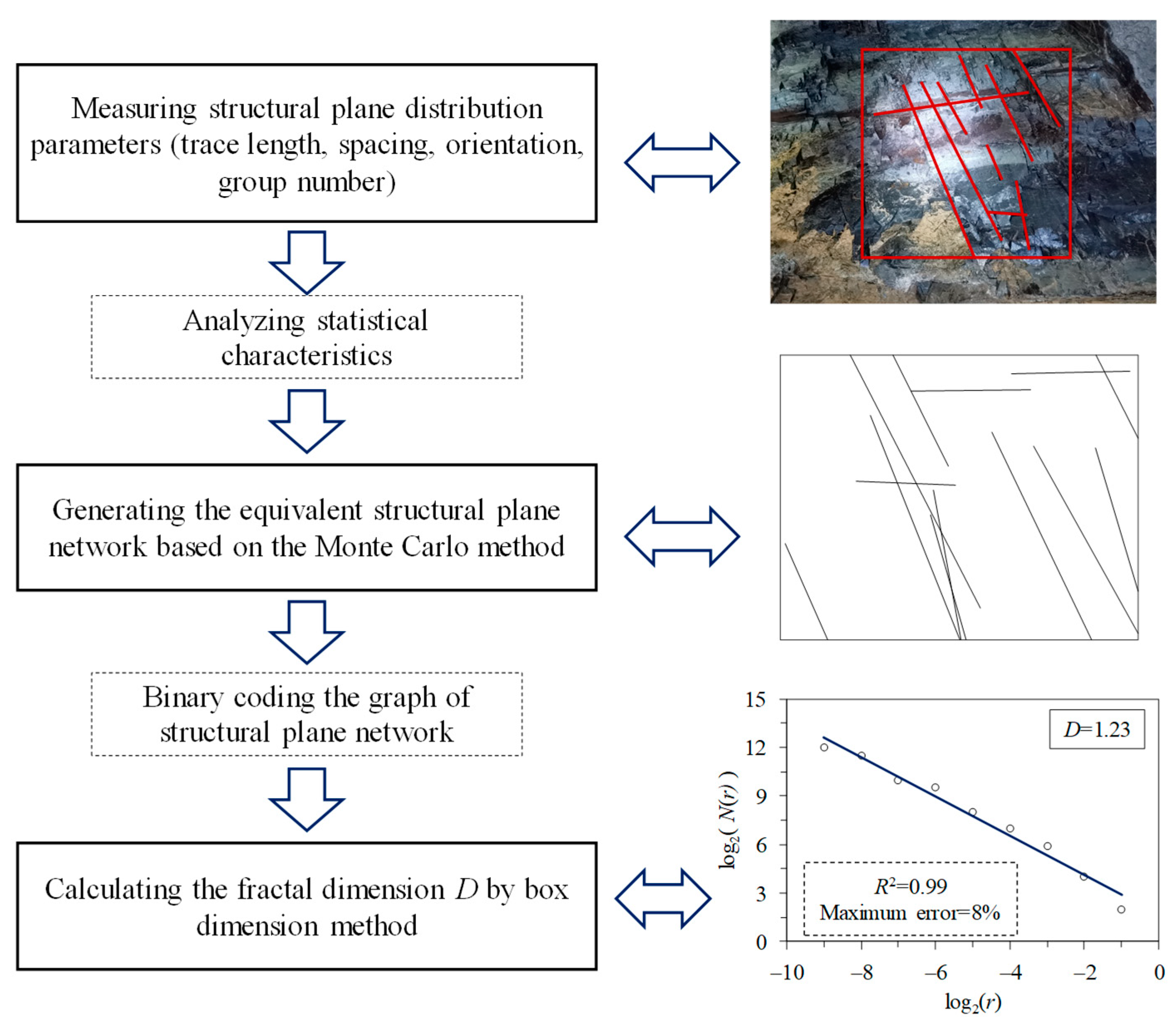
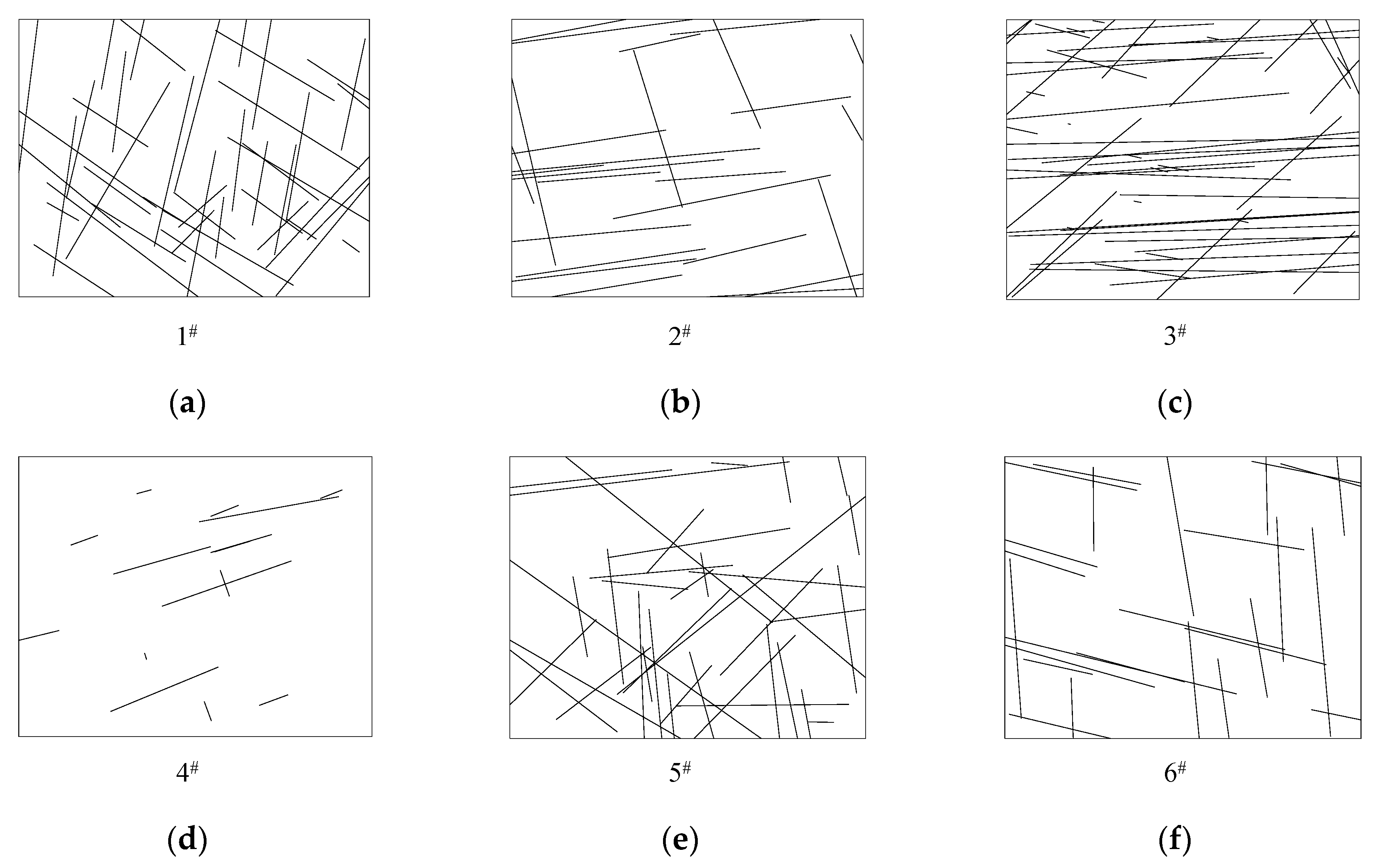
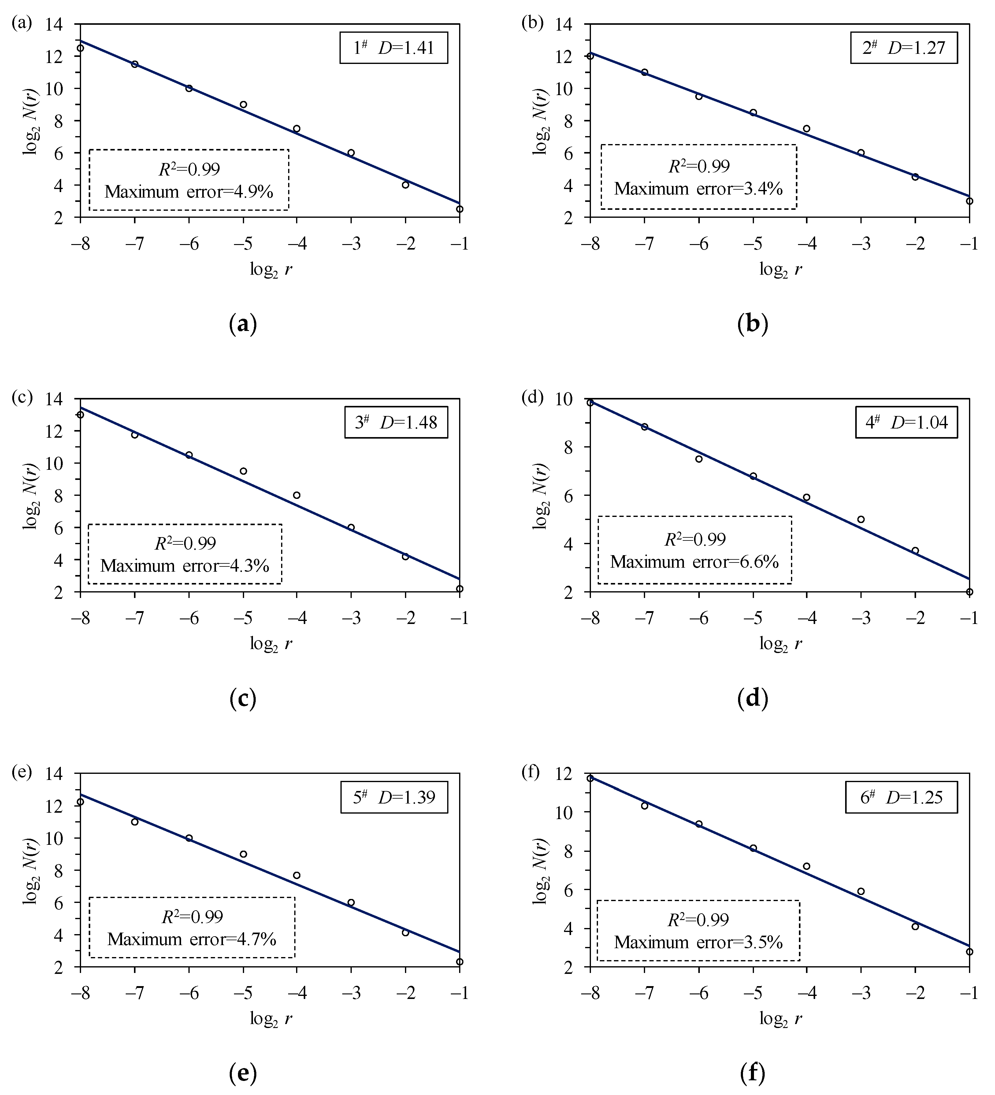
2.3. Determination of Fractal Dimension D Based on Structural Plane Network Simulation

It is difficult to determine the fractal dimension D directly in the field because the determination of the fractal dimension D requires measurements and calculations on different scales for the same object. A viable method is to generate the structural plane network of the rock mass by manual drawing or computer simulation based on the actual measured data. Numerous studies have shown that the parameters reflecting the structural plane distribution, such as spacing, trace length, dip direction, and dip angle, obey a probability distribution [54,55,56,57]. Based on the statistical characteristics of the structural plane distribution parameters, the equivalent structural plane network of the rock mass can be generated by using the Monte Carlo method [58,59,60,61]. The fractal dimension D can be calculated by applying the box-counting method to the equivalent structural plane networks.

According to the above, the measurement and calculation of the fractal dimension D of the structural plane network can be divided into three steps, and the flow chart for determining the fractal dimension D is shown in Figure 1.

• Measurements of the structural plane distribution parameters

The window measurement method is used to determine the structural plane distribution parameters recommended by the International Society for Rock Mechanics, Commission for Standardization of Laboratory and Field Tests [62]. The measurement parameters include trace length, spacing, direction, and group number. Then, these structural plane distribution parameters are analyzed to obtain the corresponding statistical characteristics.

2.

Generation of the equivalent structural plane network

Based on the statistical characteristics of the structural plane distribution parameters, a two-dimensional (2D) equivalent structural plane network is generated using the Monte Carlo method. Since the information on the structural plane distribution parameters commonly obtained in engineering measurements is 2D, and the joints of structural planes of the rock masses generally lie on a 2D sampling window. It is acceptable to consider the problem using a 2D model [30].

3.

Calculation of the fractal dimension D

The box-counting method mentioned in Section 2.1 is applied to calculate the fractal dimension D of the equivalent structural plane network. The graph of the structural plane network is generated by computer simulation and only contains structural plane information. There is no need for smoothing, sharpening, or noise removal on the graph. The graph of the equivalent structural plane network is converted to a binary representation, and the binary representation of the structural plane network is input into the Fraclab toolbox in MATLAB to calculate the fractal dimension D [63]. The Fraclab automatically selects the upper and lower limits of meshing based on the graph and calculates the fractal dimension D according to the scale range.

3. Correlation of Fractal Dimension D with Integrity Index K_v

There is a good correlation between the fractal dimension D and the indices responding to the structural characteristics of the rock mass [30,33,39,40]. The integrity index K_v, as a structural plane index in the CHN-BQ method, is closely related to the fractal dimension D. Therefore, the geological information (including structural plane distribution parameters and rock integrity index K_v) of 80 sampling windows is collected. The fractal dimension D is calculated from the structural plane distribution parameters to explore the relationship between D and K_v in this section.

3.1. Acquisition and Treatment of Structural Plane Distribution Parameters

The information collection site is located in the Mingtang Tunnel, Anhui Province, China. The geological condition of the tunnel is complex, including faulted and broken zones. The window measurement method (5 m × 5 m) is used to determine the structural plane distribution parameters in the Mingtang Tunnel. The structural plane distribution parameters are analyzed to obtain their statistical characteristics, where the trace length is a lognormal distribution, the direction (the angle between the trace and the horizontal axis of the statistics window) is a normal distribution, and the spacing is a negative exponential distribution. A total of 80 sampling windows are used to collect structural plane distribution parameters. For brevity,

Table 1. Statistical characteristics of structural plane distribution of 6 sampling windows.

No.	Number of Dominant Set (Amount)	Dominant Set	Direction (Normal Distribution)		Trace Length (Lognormal Distribution)		Spacing (Negative Exponential Distribution) (m)
			Mean (°)	Standard Deviation (°)	Mean (m)	Standard Deviation (m)
1#	3	1	138.93	3.18	1.70	0.95	0.228
		2	52.71	3.22	1.81	1.10	0.670
		3	81.34	1.67	1.99	0.67	0.292
2#	2	1	9.30	2.85	2.69	1.46	0.258
		2	107.71	4.73	2.20	1.19	0.755
3#	4	1	114.07	4.61	0.63	1.00	1.435
		2	49.18	2.52	2.62	1.12	0.384
		3	165.36	2.61	0.58	0.82	0.316
		4	3.70	3.11	5.54	0.60	0.223
4#	2	1	105.74	4.27	0.81	1.12	1.460
		2	21.51	4.05	1.11	1.13	0.419
5#	4	1	135.06	3.47	4.71	1.14	0.920
		2	9.40	2.79	3.22	1.07	0.997
		3	48.80	3.72	2.15	1.16	0.551
		4	96.11	2.78	2.18	1.40	0.324
6#	2	1	161.87	3.60	2.17	1.00	0.338
		2	93.62	3.28	2.71	0.83	0.471

^# Number of the sampling window.

only lists the results of six sampling windows, and the processing procedure for the results of the other 74 sampling windows is similar to that of the six sampling windows.

The following is the processing procedure for the results of the 80 sampling windows, using the 6 sampling windows in Table 1 as examples. Firstly, the statistical characteristics of the structural plane distribution are obtained based on the measured data from the sampling window. The equivalent structural plane networks are generated using the Monte Carlo method based on the statistical characteristics, as shown in Figure 2. The graph of the equivalent structural plane network is binary converted, and then the fractal dimension D is calculated using the box-counting method, whose grid size is 1/2~1/256. The relationship between the measurement scale r and the number of measurements N(r) is obtained and presented in Figure 3, and the absolute value of its slope is the fractal dimension D. The correlation coefficient R² and the maximum error are also presented in Figure 3. It can be found that log₂ r − log₂ N(r) is approximately linear, and the correlation coefficient R² is as high as 0.99. The maximum error is only 6.6%, which indicates that the structure-plane distribution has excellent self-similarity and fractal characteristics.

Moreover, it can be found that the larger fractal dimension D corresponds to the more fractured rock mass. For example, the 3^# equivalent structural plane network is the most fractured among the 6 equivalent structural plane networks, and its fractal dimension D is 1.48. The 4^# equivalent structural plane network is the most intact, and its fractal dimension D is only 1.04. Therefore, this also proves that the structural planes of the rock mass have significant fractal characteristics, and the fractal dimension D can accurately reflect the structural plane distribution of the rock mass.

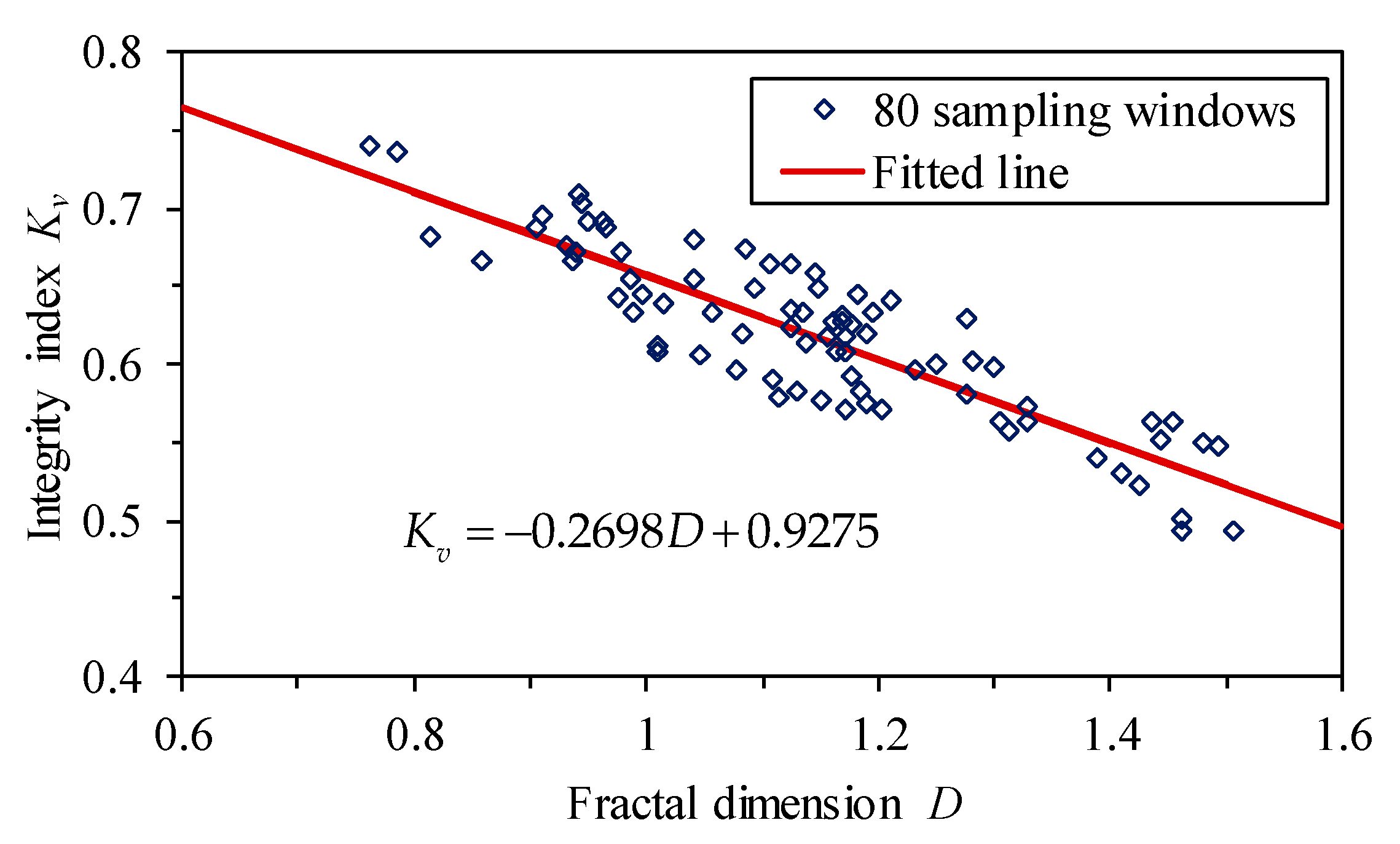
3.2. Quantitative Correlation between D and K_v

The acoustic wave test method is used to obtain the rock integrity index K_v for the 80 sampling windows. The fractal dimensions D of the 80 sampling windows are calculated according to the above process. The correlation between the fractal dimension D and the integrity index K_v is expressed in Figure 4. The quantitative correlation between D and K_v is shown in Equation (3), and the correlation coefficient R² is 0.78.

$$K_v=-0.2698D+0.9275$$

(3)

The maximum relative error between D and K_v is 8.21%, which shows that the fractal dimension D has a good correlation with the rock integrity index K_v. In addition, K_v decreases with the increase of D, which is consistent with the above finding that the larger fractal dimension D corresponds to a more fractured rock mass. The fractal dimension D contains rich information on the rock mass, which can effectively reflect the integrity, uniformity, and other characteristics of the rock mass.

The qualitative classification of rock mass integrity can be divided into five categories based on K_v (see

Table 2. Rock mass integrity classification according to K_v and D.

Rock Mass Integrity	Intact	Less Intact	Less Fractured	Fractured	Very Fractured
Integrity index Kv	>0.75	0.75~0.55	0.55~0.35	0.35~0.15	≤0.15
Fractal dimension D	<0.66	0.65~1.40	1.40~2.14	2.14~2.88	≥2.88

). According to Equation (3), the rock mass integrity can be determined directly according to fractal dimension D. The correspondence between the fractal dimension D and the rock mass integrity is listed in Table 2. Therefore, by measuring the structural plane distribution parameters and analyzing their statistical characteristics, fractal dimension D can be obtained to directly evaluate the rock mass integrity. When D is less than 0.66, the rock mass is intact, and when D is larger than 2.88, the rock mass is very fractured.

However, Figure 4 shows that the same D corresponds to different K_v because the K_v is also related to the structural plane conditions (such as infilling, weathering, and aperture). In addition, the above quantitative correlation is only from the field data of one project, which is not a universal quantitative relationship between D and K_v. Therefore, more data from different rock mass engineering methods and consideration of structural plane conditions are needed to acquire a more accurate method for determining K_v.

4. Prediction of K_v by BP Neural Network

In essence, the relationship between the integrity index K_v and the fractal dimension D, considering the structural plane conditions, is a regression problem that can be solved by the ANN. ANN is a common mathematical model in machine learning that can process information under uncertainty based on prior experience by constructing brain-like neural structures. The back-propagation (BP) neural network is a notable method [41], which consists of the input layer, hidden layer, and output layer. The input layer receives signals and data from outside; the output layer realizes the output of the system processing results; and the hidden layer is between the input and output units and can be one or more layers whose structure is not observable from outside the network. Each layer is composed of different neurons that are connected to the neurons of the next layer. The strength of the connection between neurons is determined by the weights and biases.

The integrity index K_v considers both the geometric characteristics of structural planes and structural plane conditions. Where the geometric characteristics of structural planes can be well quantified by the fractal dimension D, and the structural plane conditions need to be quantitatively assessed with the help of other rock mass classifications. The structural plane condition index (R₃) in the RMR₁₄ [64], which considers continuity, roughness, infilling, and weathering, can well represent the structural plane condition of the rock mass. Therefore, the BP neural network is constructed with the fractal dimension D and the structural plane condition index R₃ in the RMR₁₄ as the two input neurons and the integrity index K_v as the output neuron. The structure of a 3-layer BP neural network for predicting K_v and its two-step calculation procedures are shown in Figure 5.

The BP neural network processes the input D and R₃ data and produces initial results in the output layer. The calculation between the input and output in the BP neural network is expressed as follows [65]:

$$y_k=f_{output}\left[{\displaystyle \sum _{j=1}^m{w}_{kj}{f}_{hidden}({\displaystyle \sum _{i=1}^n{W}_{ji}{x}_i}+b_j^h)+b_k^o}\right]$$

(4)

where x_i is the i-th input vector of the BP neural network (i = 1, 2, …, n), y_k is the k-th output vector of the BP neural network (k = 1, 2, …, n); $b_j^h$ and $b_k^o$ are the biases of hidden and output layers; f_output and f_hidden are the respective transfer functions for the hidden and output neurons; w_ji is the weight vector from the input layer to hidden layer (j = 1, 2, …, m) and W_kj are the weight vector from the hidden layer to output layer (k = 1, 2, …, l); n, m, and l are the neurons of input, hidden, and output layers, respectively.

The output vector y_k is different from the target vector y_k′ (the initial input data). The mean square error (E_k) between the two vectors is calculated by Equation (5). If the mean square error exceeds the minimum threshold, the weights and biases will be modified, and the output results will be retrained according to the modified weights and biases. The above calculation procedure is repeated until the mean square error of the output results is within the minimum threshold.

$$E_k=\frac{1}{2}{{\displaystyle \sum (y_k{}^{\prime }-y_k)}}^2$$

(5)

where y_k′ is the target vector that is input initially, and y_k is the output vector calculated by the BP neural network. E_k is the mean square error between them.

The BP neural network is programmed in MATLAB. The learning dataset involves 260 groups of data collected from the excavation faces of six tunnels [66], including 80 groups of data from the Mingtang Tunnel applied in Section 2. 15% of the 260 data points are randomly selected as the test data, so 39 of the 260 data points are used to test the performance of the BP neural network. The number of hidden neurons is set to 10. The transfer function is the “trainbr”, which updates weight and bias values by Bayesian regularization. It minimizes the combination of squared errors and weights and determines the correct combination to produce a well-generalized network [67,68]. Because the training data set is small, this algorithm can produce good generalizations and avoid overfitting. Figure 6 shows the change in the mean squared error according to the learning iteration. It can be found that after the epoch is greater than 10, the mean squared error remains unchanged. The BP neural network is trained for 96 epochs, and the best training performance is at epoch 33 with a mean squared error of 0.0022485.

In the BP neural network for predicting K_v, the output is the predicted K_vp, and the target is the measured K_vm. After training 96 epochs, the errors between the targets K_vm and the outputs K_vp for training data and test data are presented as the error histogram in Figure 7. It can be found that the errors for the training data are mainly distributed in −0.1439~0.08529, and the most distributed error is 0.01477. The errors for the training data are distributed in −0.1087~0.06766, and the most distributed error is −0.00286. The errors in the training data and test data are mostly around zero.

Figure 8 shows the regression of the training and test data for the BP neural network. The correlation coefficient R² between the targets and outputs is 0.89 for the training data and 0.94 for the test data, which means that the targets are highly related to the output. The fitted line is close to the K_vp = K_vm line, and when K_v is small, the fitted K_vp is slightly larger than the K_vm, while when K_v is large, the fitted K_vp is almost the same as the K_vm, especially for the test data. Moreover, the average relative error for the test data is 7.51%. To sum up, the BP neural network is well trained, and the K_vp predicted by the fractal dimension D and the structural plane condition index R₃ through the BP neural network is in high agreement with the measured K_vm.

To further explore the advantages of predicting K_v by the BP neural network compared to directly predicting K_v by fractal dimension D, K_vd for 39 test data is obtained based on the quantitative correlation between D and K_v in Section 3. The specific values are listed in

Table 3. Comparison of K_v obtained by the BP neural network and fractal dimension D with the measured K_v.

No.	Integrity Index Kv			Relative Error (%)
	Kvm	Kvp	Kvd	Kvm − Kvp	Kvm − Kvd
1	0.07	0.10	0.41	51.05	519.22
2	0.14	0.13	0.43	4.81	220.35
3	0.15	0.17	0.44	7.42	187.59
4	0.28	0.24	0.43	15.52	55.44
5	0.29	0.31	0.48	4.67	63.85
6	0.34	0.33	0.48	2.70	42.56
7	0.36	0.42	0.52	16.31	43.86
8	0.37	0.48	0.45	29.12	23.33
9	0.38	0.35	0.46	7.86	21.32
10	0.38	0.39	0.50	2.99	30.99
11	0.45	0.45	0.50	0.51	11.91
12	0.46	0.46	0.53	0.00	16.12
13	0.46	0.50	0.50	7.91	7.53
14	0.46	0.45	0.49	3.93	6.10
15	0.47	0.49	0.52	4.34	10.06
16	0.49	0.49	0.50	0.46	2.49
17	0.49	0.47	0.53	4.64	7.06
18	0.52	0.63	0.52	22.53	0.87
19	0.53	0.52	0.56	1.74	6.18
20	0.54	0.58	0.59	5.87	8.36
21	0.57	0.60	0.61	6.01	7.81
22	0.57	0.57	0.56	1.19	1.57
23	0.58	0.54	0.54	6.74	6.83
24	0.60	0.54	0.55	9.91	8.63
25	0.60	0.52	0.59	14.05	2.04
26	0.60	0.69	0.68	15.13	13.13
27	0.62	0.58	0.65	5.92	6.23
28	0.64	0.65	0.65	2.15	1.93
29	0.64	0.74	0.57	14.87	11.97
30	0.68	0.65	0.67	3.70	1.39
31	0.68	0.72	0.70	5.33	2.91
32	0.70	0.69	0.59	0.98	15.11
33	0.72	0.74	0.68	2.54	5.21
34	0.73	0.71	0.65	2.19	10.52
35	0.72	0.74	0.61	3.36	15.94
36	0.72	0.74	0.62	1.93	14.39
37	0.73	0.72	0.65	0.57	10.18
38	0.74	0.74	0.67	0.10	9.29
39	0.74	0.75	0.74	1.89	0.08
Average				7.51	36.68

, and the correlation between K_vd, K_vp, and K_vm is shown in Figure 9. The average relative error is 7.51% for K_vp and K_vm, while the average relative error for K_vd and K_vm is 36.68%. When K_vm is less than 0.5, the K_vd obtained by fractal dimension D is much larger than the measured K_vm. The K_vp predicted by the BP neural network is similar to the measured K_vm in the whole range. It can be found that the inclusion of the R₃ significantly improves the accuracy of predicting K_v, especially in the case of K_v > 0.5. Comparing the weights of the two inputs of the BP neural network after training can further explore the effect of R₃ on the prediction accuracy of K_v. Since there are 10 hidden neurons, the weights w_ji of the two inputs are two vectors, expressed as follows:

$$\left[\begin{array}{l}-0.1101\\ -0.3288\\ -0.1303\\ -0.0383\\ 0.2417\\ 0.3374\\ 1.4981\\ -0.1532\\ -0.1059\\ -0.1729\end{array}\right]\mathrm{for}D\mathrm{and}\left[\begin{array}{l}0.0212\\ -0.2095\\ 0.0637\\ 0.0532\\ -0.1611\\ 0.6731\\ 0.0001\\ 0.0411\\ 0.0783\\ 0.0290\end{array}\right]\mathrm{for}{R}_3$$

(6)

Adding up each value of the two weight vectors reveals that the weight of D is 1.0377, and the weight of R₃ is 0.5891. The two inputs of D and R₃ have been normalized, so it can be found that the effect of R₃ on K_v is about half that of D. To sum up, the BP neural network for prediction K_v, which considers both geometric characteristics of structural planes and structural plane conditions, is more accurate than the fractal dimension D in the determination of K_v.

5. Application of BP Neural Network for Predicting K_v in Jiulaopo Tunnel

The BP neural network for predicting K_v is applied in the Jiulaopo Tunnel, located in Guizhou Province, China. The highest elevation of the site is 853.6 m, the lowest elevation is 471.4 m, and the relative maximum elevation difference is 382.2 m. It is located in the South China Fold Belt, dominated by north- or northeast-oriented belt folds. No faults pass through the tunnel, and the stratigraphy is smooth. The surrounding rock of the tunnel is gravelly chalky clay and medium-weathered tuff slate; the rock is relatively intact. Groundwater is greatly influenced by the seasons. In the rainy season, bedrock fracture water is abundant and large, and in the dry season, recharge is poor and the volume is small. The water quality type at the site is calcium carbonate water, and the groundwater is slightly corrosive to the concrete structure. Figure 10 shows the construction site and excavation face of the Jiulaopo Tunnel. The measured K_vm is tested by the acoustic wave test. The structural plane distribution parameters are obtained by the window measurement method, and their statistical characteristics are summarized. Only one sampling window is taken for each excavation face. The structural plane condition index R₃ is assessed according to the RMR₁₄ classification. Based on the statistical characteristics of the structural plane distribution parameters, the fractal dimension D is obtained and further combined with R₃ to predict K_vp by the BP neural network.

Table 4. Measured and predicted integrity index K_v for 10 sampling windows.

No.	Rating in R3					Structural Plane Distribution Parameters							Integrity Index Kv
	Continuity	Roughness	Infilling	Weathering	R3	Number of Dominant Set (Amount)	Direction		Trace Length		Spacing (m)	D	Kvp	Kvm	Relative Error (%)
							Mean (°)	Standard Deviation (°)	Mean (m)	Standard Deviation (m)
a	4	3	5	3	15	1	64.29	1.43	2.90	1.39	0.09	1.74	0.37	0.39	5.13
b	4	2	2	6	14	2	48.06	2.60	1.08	0.72	1.85	1.01	0.68	0.65	4.62
							82.13	1.65	0.70	0.49	1.12
c	4	3	2	1	10	2	26.00	4.58	1.71	0.61	1.58	1.10	0.63	0.63	0
							101.09	1.51	1.51	1.12	0.58
d	2	1	4	1	8	1	83.45	1.40	2.07	0.95	0.41	1.21	0.58	0.59	1.69
e	5	3	5	5	18	1	67.55	3.48	0.89	0.62	1.12	0.93	0.71	0.68	4.41
f	4	2	0	0	6	1	73.27	2.40	2.25	0.66	0.79	1.07	0.59	0.58	1.72
g	5	5	4	3	17	2	16.01	2.84	4.80	1.12	1.49	1.06	0.69	0.67	2.99
							59.35	4.60	1.11	1.41	0.4
h	2	3	2	1	8	1	66.06	3.06	3.70	1.12	0.203	1.36	0.54	0.56	3.57
i	4	1	5	1	11	3	55.82	1.87	4.33	0.99	0.591	1.27	0.60	0.60	0
							7.03	4.43	4.49	1.10	1.009
							82.43	3.16	3.66	0.87	0.671
j	5	3	2	0	10	1	16.22	4.68	0.89	0.85	1.120	0.86	0.65	0.67	2.99

presents the measured and predicted K_v for the 10 sampling windows. The structural plane distribution parameters for the 10 sampling windows are similarly listed. It can be found that the K_vm for these 10 sampling windows varies between 0.39 and 0.68, and the K_vp predicted by the BP neural network varies between 0.37 and 0.71. The maximum relative error between the predicted K_vp and measured K_vm is 5.13%, and the average relative error is 2.71%. Such a small error implies that the prediction of K_v by the BP neural network based on the fractal dimension D and structural plane index R₃ is accurate.

After simply measuring the distribution characteristics of the structural planes and rating their conditions according to R₃ in rock mass engineering, the integrity index K_v can be accurately determined by the BP neural network. The method uses parameters that are convenient to obtain and takes into account the geometric properties of the structural planes and structural plane conditions. In summary, predicting K_v by the BP neural network can reduce the empirical judgment of parameter taking and make an accurate quantitative estimation of K_v.

6. Discussions

The determination of K_v by the BP neural network requires parameters about structural plane distribution and structural plane conditions. These parameters can be obtained by precise quantitative evaluation methods, such as the window measurement method and the R₃ rating of RMR₁₄. The precise quantitative evaluation methods improve the accuracy of parameter acquisition and avoid the ambiguous situation of empirical judgment. For practitioners lacking engineering experience, the geological information can be quickly determined in complex construction environments, and thus the integrity index K_v can be accurately determined. Apart from the convenience and accuracy of the parameter acquisition, the determination of K_v by the BP neural network comprehensively considers the geometric characteristics of structural planes and structural plane conditions, which significantly improves the accuracy of predicting K_v.

However, there is much improvement in this method. The fractal dimension D is obtained by 2D structural plane network simulation. Although the 2D model can represent some structural plane characteristics of the rock mass, it still differs from the 3D structural plane of the real rock mass. Therefore, researchers have proposed the method of 3D structural plane network simulation [21,57,69], such as inferring the 3D structural plane distribution based on 2D geological information [70,71,72]. The simulated 3D structural plane network has a better correspondence with the real rock structural plane, and the equivalent 3D structural plane network can effectively reduce the randomness of the 2D structural plane network. The subsequent research can obtain the fractal dimension D by 3D structural plane network simulation.

Additionally, with the development of graphic recognition technology [30,36,73], fractal dimension D can be rapidly obtained from images without measuring the structural plane distributions. This method determines the fractal dimension D directly from real rock images, which is more accurate than the fractal dimension D from the equivalent structural surface network generated by simulation. The precision of this method depends on the quality of the rock image, which usually requires processing such as noise removal and smoothing of the image. Determining the fractal dimension D and thus K_v from the real rock images is also one of the directions of the subsequent research.

7. Conclusions

In this study, a new quantitative evaluation of the integrity index K_v by the BP neural network based on the fractal dimension D is proposed, and the applicability of the method is verified with an example of rock mass engineering. Conclusions are drawn as follows:

• The fractal dimension D correlates well with the integrity index K_v, with a maximum relative error of 8.21%. Meanwhile, the larger fractal dimension D corresponds to the smaller K_v and the more fractured rock mass. The fractal dimension D of the structure plane contains rich information on the rock mass, and it can effectively reflect the integrity, uniformity, and other characteristics of the rock mass.
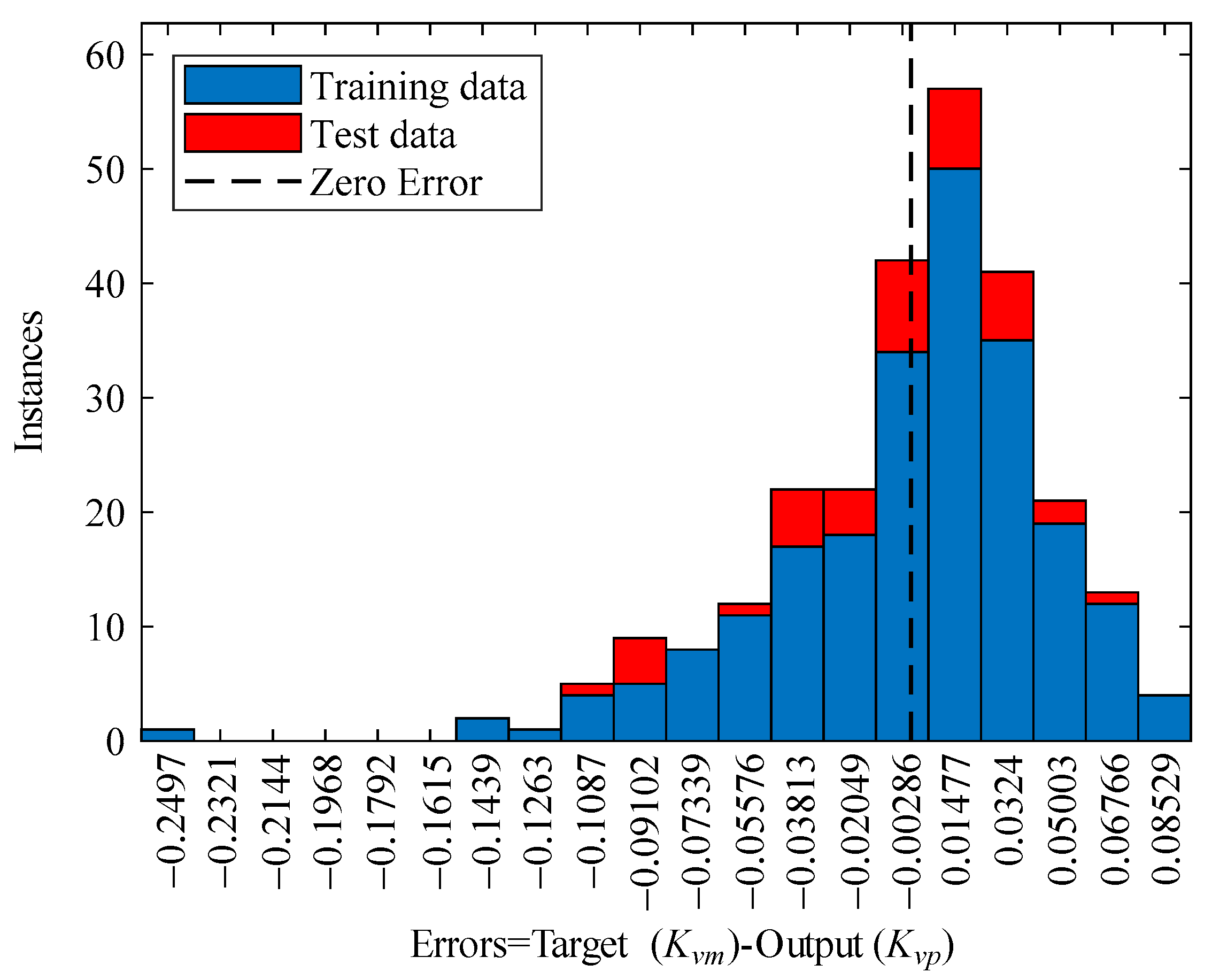
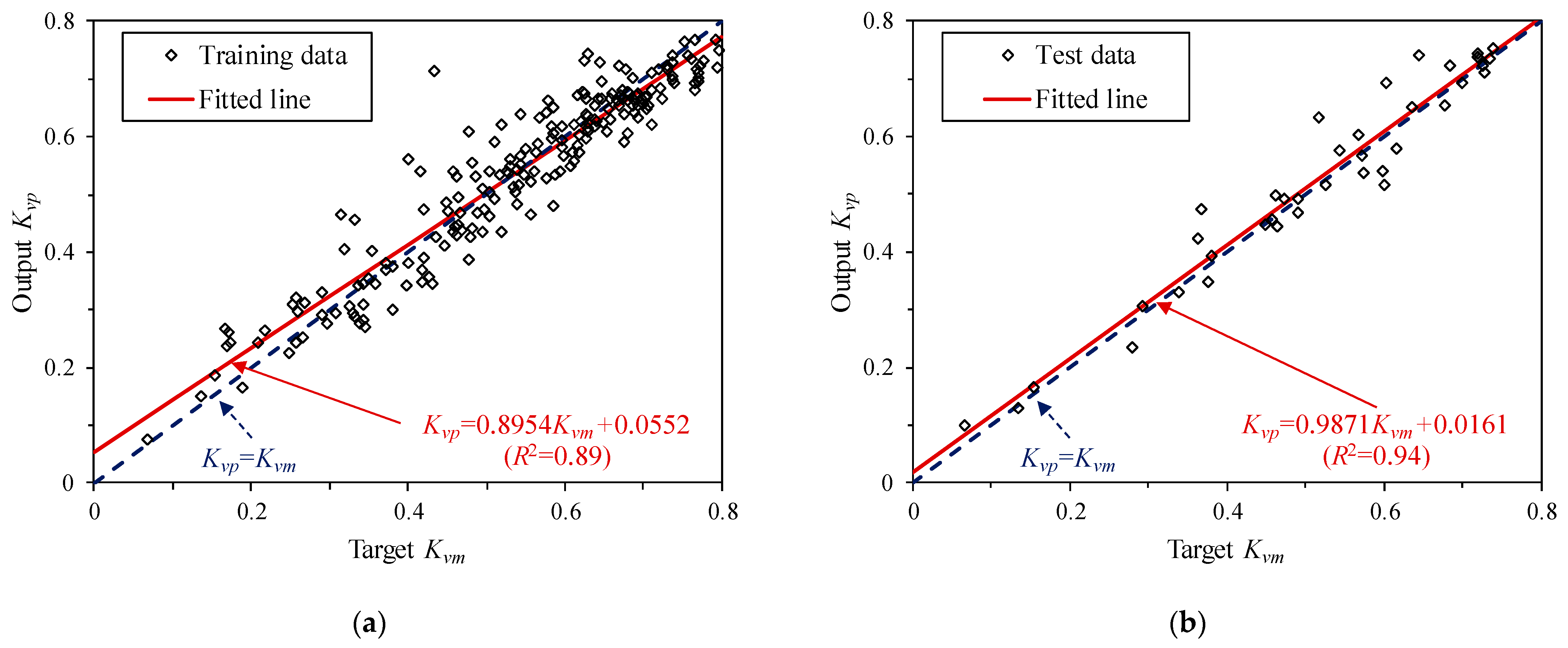
• The BP neural network for predicting K_v is well trained. The correlation coefficient R² between the predicted K_vp by the BP neural network and the measured K_vm is 0.93, and the average relative error is 7.51%. Compared with the K_vd determined directly by fractal dimension D, there is a large error in K_vd, especially when K_v is less than 0.5. The BP neural network for predicting K_v, which considers both geometric characteristics of structural planes and structural plane conditions, is more accurate than determining K_v by fractal dimension D.
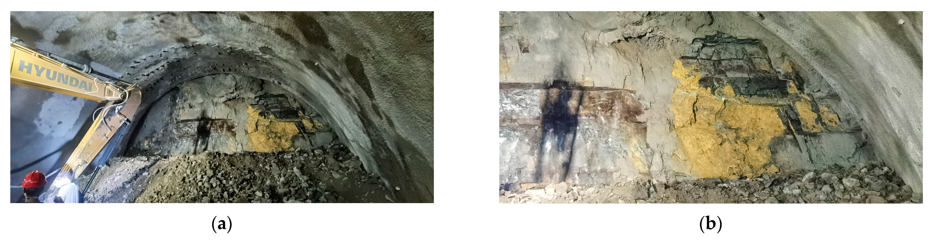
• The BP neural network for predicting K_v is applied to the Jiulaopo Tunnel. The maximum relative error between the measured K_vm and the predicted K_vp is 5.13%, and the average relative error is 2.71% for the 10 sampling windows. It shows that the BP neural network for predicting K_v performs well in rock engineering and can predict K_v accurately.

The method of predicting K_v by the BP neural network proposed in this study is an accurate quantitative evaluation of K_v with convenient parameter acquisition and consideration of the geometric properties and structural plane conditions. This method is objective and does not require rich experience. It can be improved by obtaining fractal dimension D through 3D structural plane network simulation and graphic recognition technology.

References

1. Singh, B.; Goel, R.K. Engineering Rock Mass Classification: Tunnelling, Foundations and Landslides; Elsevier: Amsterdam, The Netherlands, 2011. [Google Scholar]
2. Zhang, L.Y. Evaluation of rock mass deformability using empirical methods—A review. Undergr. Space 2017, 2, 1–15. [Google Scholar] [CrossRef]
3. Deere, D.U. Technical description of rock cores for engineer purposes. Rock Mech. Eng. Geol. 1964, 1, 17–22. [Google Scholar]
4. Barton, N.; Lien, R.; Lunde, J. Engineering classification of rock masses for the design of tunnel support. Rock Mech. Rock Eng. 1974, 6, 189–236. [Google Scholar] [CrossRef]
5. Brown, E.; Hoek, E. Strength of rock and rock masses. ISRM News J. 1994, 2, 4–16. [Google Scholar]
6. Hoek, E.; Kaiser, P.; Bawden, W. Support of Underground Wxcavations in Hard Rock; A. A. Balkema: Rotterdam, The Netherlands, 1995. [Google Scholar]
7. Bieniawski, Z.T. Engineering classification of jointed rock masses. Civ. Eng. S. Afr. 1973, 15, 333–343. [Google Scholar]
8. Bieniawski, Z.T. Engineering Rock Mass Classifications: A Complete Manual for Engineers and Geologists in Mining, Civil, and Petroleum Engineering; John Wiley and Sons: New York, NY, USA, 1989. [Google Scholar]
9. Wu, A.Q.; Zhao, W.; Zhang, Y.H.; Fu, X. A detailed study of the CHN-BQ rock mass classification method and its correlations with RMR and Q system and Hoek-Brown criterion. Int. J. Rock Mech. Min. Sci. 2023, 162, 105290. [Google Scholar] [CrossRef]
10. Shen, Y.-J.; Yan, R.-X.; Yang, G.-S.; Xu, G.-L.; Wang, S.-Y. Comparisons of Evaluation Factors and Application Effects of the New [BQ]GSI System with International Rock Mass Classification Systems. Geotech. Geol. Eng. 2017, 35, 2523–2548. [Google Scholar] [CrossRef]
11. Cui, Z.; Sheng, Q.; Zhang, G.-M.; Liu, H. A modified rock mass classification considering seismic effects in the basic quality (BQ) system. Bull. Eng. Geol. Environ. 2021, 80, 2249–2260. [Google Scholar] [CrossRef]
12. Wu, A.Q.; Liu, F.Z. Advancement and application of the standard of engineering classification of rock masses. Chin. J. Rock Mech. Eng. 2012, 31, 1513–1523. [Google Scholar]
13. Shen, Y.J.; Yang, G.S.; Yan, R.X. Revised BQ system in China and its correlation to international rock mass classification systems. In Proceedings of the World Mining Congress, Canadian Institute of Mining, Metallurgy and Petroleum, Montreal, QC, Canada, 11–15 August 2013. [Google Scholar]
14. Yan, R.X.; Shen, Y.J. Correlation of revised BQ system in China and the international rock mass classification systems. J. Civ. Eng. Res. 2015, 5, 33–38. [Google Scholar]
15. Zhou, F.J.; Chen, J.P.; Xu, L.M. Study of rock masses quality evaluation based on 3D fractal dimension of rock discontinuity distribution. Rock Soil Mech. 2012, 33, 2315–2322. [Google Scholar]
16. Ghosh, A.; Daemen, J.J. Fractal characteristics of rock discontinuities. Eng. Geol. 1993, 34, 1–9. [Google Scholar] [CrossRef]
17. Sun, S.Q.; Li, S.C.; Li, L.P.; Shi, S.S.; Liu, H.L.; Hu, J.; Zhou, S. Structural planes surveying and fractal dimension characteristics of tunnel face based on digital photogrammetry. Arab. J. Geosci. 2018, 11, 622. [Google Scholar] [CrossRef]
18. Bagde, M.; Raina, A.; Chakraborty, A.; Jethwa, J. Rock mass characterization by fractal dimension. Eng. Geol. 2002, 63, 141–155. [Google Scholar] [CrossRef]
19. Ehlen, J. Fractal analysis of joint patterns in granite. Int. J. Rock Mech. Min. Sci. 2000, 37, 909–922. [Google Scholar] [CrossRef]
20. La Pointe, P. A method to characterize fracture density and connectivity through fractal geometry. Int. J. Rock Mech. Min. Sci. Géoméch. Abstr. 1988, 25, 421–429. [Google Scholar] [CrossRef]
21. Zhao, Y.; Feng, Z.; Dong, Y.; Liang, W.; Feng, Z. Three-dimensional fractal distribution of the number of rock-mass fracture surfaces and its simulation technology. Comput. Geotech. 2015, 65, 136–146. [Google Scholar] [CrossRef]
22. Xie, H.; Wang, J.-A.; Xie, W.-H. Fractal effects of surface roughness on the mechanical behavior of rock joints. Chaos Solitons Fractals 1997, 8, 221–252. [Google Scholar] [CrossRef]
23. Lee, Y.-H.; Carr, J.R.; Barr, D.J.; Haas, C.J. The fractal dimension as a measure of the roughness of rock discontinuity profiles. Int. J. Rock Mech. Min. Sci. Géoméch. Abstr. 1990, 27, 453–464. [Google Scholar] [CrossRef]
24. Nayak, S.R.; Mishra, J.; Palai, G. Analysing roughness of surface through fractal dimension: A review. Image Vis. Comput. 2019, 89, 21–34. [Google Scholar] [CrossRef]
25. Brown, S.R. A note on the description of surface roughness using fractal dimension. Geophys. Res. Lett. 1987, 14, 1095–1098. [Google Scholar] [CrossRef]
26. Li, Y.R.; Huang, R.Q. Relationship between joint roughness coefficient and fractal dimension of rock fracture surfaces. Int. J. Rock Mech. Min. Sci. 2015, 75, 15–22. [Google Scholar] [CrossRef] [Green Version]
27. Hirata, T.; Satoh, T.; Ito, K. Fractal structure of spatial distribution of microfracturing in rock. Geophys. J. Int. 1987, 90, 369–374. [Google Scholar] [CrossRef]
28. Xie, H.P.; Liu, J.F.; Ju, Y.; Li, J.G.; Xie, L.Z. Fractal property of spatial distribution of acoustic emissions during the failure process of bedded rock salt. Int. J. Rock Mech. Min. Sci. 2011, 48, 1344–1351. [Google Scholar] [CrossRef]
29. Li, W.; Zhao, H.; Wu, H.; Wang, L.; Sun, W.; Ling, X. A novel approach of two-dimensional representation of rock fracture network characterization and connectivity analysis. J. Pet. Sci. Eng. 2019, 184, 106507. [Google Scholar] [CrossRef]
30. Hong, K.; Han, E.; Kang, K. Determination of geological strength index of jointed rock mass based on image processing. J. Rock Mech. Geotech. Eng. 2017, 9, 702–708. [Google Scholar] [CrossRef]
31. Carr, J.R.; Wardner, J.B. Rock mass classification using fractal dimension. In Proceedings of the 28th US Symposium on Rock Mechanics (USRMS), Tucson, AZ, USA, 29 June–1 July 1987. [Google Scholar]
32. Hamdi, E.; du Mouza, J. A methodology for rock mass characterisation and classification to improve blast results. Int. J. Rock Mech. Min. Sci. 2005, 42, 177–194. [Google Scholar] [CrossRef]
33. Lian, J.F.; Shen, N.Q.; Zhang, J.K. Application research on fractal theory in rockmass quality evaluation. Chin. J. Rock Mech. Eng. 2001, 20, 1695–1698. [Google Scholar]
34. Liu, Y.Z.; Sheng, J.L.; Ge, X.R.; Wang, S.L. Evaluation of rock mass quality based on fractal dimension of rock mass discontinuity distribution. Rock Soil Mech. 2007, 28, 971–975. [Google Scholar]
35. Liebovitch, L.S.; Toth, T. A fast algorithm to determine fractal dimensions by box counting. Phys. Lett. A 1989, 141, 386–390. [Google Scholar] [CrossRef]
36. Zhang, Y.Z.; Ji, H.G.; Li, W.G.; Hou, K.K.; Hao, X.J. Research on Rapid Evaluation of Rock Mass Quality Based on Ultrasonic Borehole Imaging Technology and Fractal Method. Adv. Mater. Sci. Eng. 2021, 2021, 8063665. [Google Scholar] [CrossRef]
37. Ai, T.; Zhang, R.; Zhou, H.W.; Pei, J.L. Box-counting methods to directly estimate the fractal dimension of a rock surface. Appl. Surf. Sci. 2014, 314, 610–621. [Google Scholar] [CrossRef]
38. Yu, B.M.; Li, J.H. Some fractal characters of porous media. Fractals 2001, 9, 365–372. [Google Scholar] [CrossRef]
39. Stigsson, M.; Ivars, D.M. A Novel Conceptual Approach to Objectively Determine JRC Using Fractal Dimension and Asperity Distribution of Mapped Fracture Traces. Rock Mech. Rock Eng. 2018, 52, 1041–1054. [Google Scholar] [CrossRef] [Green Version]
40. Sanei, M.; Faramarzi, L.; Goli, S.; Fahimifar, A.; Rahmati, A.; Mehinrad, A. Development of a new equation for joint roughness coefficient (JRC) with fractal dimension: A case study of Bakhtiary Dam site in Iran. Arab. J. Geosci. 2015, 8, 465–475. [Google Scholar] [CrossRef]
41. Liu, B.; Wang, R.; Zhao, G.; Guo, X.; Wang, Y.; Li, J.; Wang, S. Prediction of rock mass parameters in the TBM tunnel based on BP neural network integrated simulated annealing algorithm. Tunn. Undergr. Space Technol. 2019, 95, 103103. [Google Scholar] [CrossRef]
42. Zhou, J.; Bejarbaneh, B.Y.; Armaghani, D.J.; Tahir, M.M. Forecasting of TBM advance rate in hard rock condition based on artificial neural network and genetic programming techniques. Bull. Eng. Geol. Environ. 2019, 79, 2069–2084. [Google Scholar] [CrossRef]
43. Lemy, F.; Hadjigeorgiou, J. Discontinuity trace map construction using photographs of rock exposures. Int. J. Rock Mech. Min. Sci. 2003, 40, 903–917. [Google Scholar] [CrossRef]
44. Sonmez, H.; Gokceoglu, C.; Nefeslioglu, H.A.; Kayabasi, A. Estimation of rock modulus: For intact rocks with an artificial neural network and for rock masses with a new empirical equation. Int. J. Rock Mech. Min. Sci. 2006, 43, 224–235. [Google Scholar] [CrossRef]
45. Zhang, Z.Q.; Wu, Q.M.; Zhang, Q.; Gong, Z.C. Estimation of Rock Mass Rating System with an Artificial Neural Network. In Proceedings of the Advances in Neural Networks—ISNN 2009: 6th International Symposium on Neural Networks, Wuhan, China, 26–29 May 2009. [Google Scholar] [CrossRef]
46. Khatik, V.M.; Nandi, A.K. A generic method for rock mass classification. J. Rock Mech. Geotech. Eng. 2018, 10, 102–116. [Google Scholar] [CrossRef]
47. He, M.M.; Zhang, Z.Q.; Li, N. Deep Convolutional Neural Network-Based Method for Strength Parameter Prediction of Jointed Rock Mass Using Drilling Logging Data. Int. J. Géoméch. 2021, 21, 04021111. [Google Scholar] [CrossRef]
48. Mandelbrot, B.B. Fractals: Form, Chance and Dimension; W. H. Freeman and Company: San Francisco, CA, USA, 1977. [Google Scholar]
49. Mandelbrot, B.B. The Fractal Geometry of Nature; W. H. Freeman and Company: New York, NY, USA, 1982; Volume 1. [Google Scholar]
50. Xie, H. Fractals in Rock Mechanics; Balkema: Rotterdam, The Netherlands, 2020. [Google Scholar]
51. Falconer, K. Fractal Geometry—Mathematical Foundations and Applications; John Wiley & Sons: New York, NY, USA, 2004. [Google Scholar]
52. Kulatilake, P.H.; Fiedler, R.; Panda, B.B. Box fractal dimension as a measure of statistical homogeneity of jointed rock masses. Eng. Geol. 1997, 48, 217–229. [Google Scholar] [CrossRef]
53. Gao, M.-Z.; Zhang, J.-G.; Li, S.-W.; Wang, M.; Wang, Y.-W.; Cui, P.-F. Calculating changes in fractal dimension of surface cracks to quantify how the dynamic loading rate affects rock failure in deep mining. J. Cent. South Univ. 2020, 27, 3013–3024. [Google Scholar] [CrossRef]
54. Wang, P. The Network Simulation of Jointed Rock Mass Discontinuities. Master’s Thesis, Tongji University, Shanghai, China, 2008. [Google Scholar]
55. Song, L.J. Description of Joint Geometry Character and Study on the Model of Joint Geometric Parameters Based on Fractal Theory. Ph.D. Thesis, Chengdu University of Technology, Chengdu, China, 2013. [Google Scholar]
56. Priest, S.D.; Hudson, J. Discontinuity spacings in rock. Int. J. Rock Mech. Min. Sci. Géoméch. Abstr. 1976, 13, 135–148. [Google Scholar] [CrossRef]
57. Dong, S.; Yi, X.; Feng, W. Quantitative Evaluation and Classification Method of the Cataclastic Texture Rock Mass Based on the Structural Plane Network Simulation. Rock Mech. Rock Eng. 2018, 52, 1767–1780. [Google Scholar] [CrossRef]
58. Chen, S.-H.; Feng, X.-M.; Isam, S. Numerical estimation of REV and permeability tensor for fractured rock masses by composite element method. Int. J. Numer. Anal. Methods Géoméch. 2008, 32, 1459–1477. [Google Scholar] [CrossRef]
59. Xu, C.; Dowd, P. A new computer code for discrete fracture network modelling. Comput. Geosci. 2013, 36, 292–301. [Google Scholar] [CrossRef]
60. Liu, R.C.; Jiang, Y.J.; Li, B.; Wang, X.S. A fractal model for characterizing fluid flow in fractured rock masses based on randomly distributed rock fracture networks. Comput. Geotech. 2015, 65, 45–55. [Google Scholar] [CrossRef] [Green Version]
61. Wu, N.; Liang, Z.Z.; Zhang, Z.H.; Li, S.H.; Lang, Y.X. Development and verification of three-dimensional equivalent discrete fracture network modelling based on the finite element method. Eng. Geol. 2022, 306, 106759. [Google Scholar] [CrossRef]
62. ISRM. Suggested methods for the quantitative description of discontinuities in rock masses. Int. J. Rock. Mech. Min. Sci. Geomech. Abstr. 1978, 15, 319–368. [Google Scholar]
63. Véhel, J.L.; Legrand, P. Signal and Image processing with FracLab. Signal and image processing with FracLab. FRACTAL04, Thinking in Patterns: Complexity and Fractals in Nature. In Proceedings of the 8th International Multidisciplinary Conference, Baia Mare, Romania, 4–6 September 2004. [Google Scholar]
64. Celada, B.; Tardáguila, I.; Varona, P.; Rodríguez, A.; Bieniawski, Z. Innovating tunnel design by an improved experience-based RMR system. In Proceedings of the World Tunnel Congress, Foz do Iguaçu, Brazil, 9–15 May 2014. [Google Scholar]
65. Hecht-Nielsen, R. Theory of the backpropagation neural network. In Proceedings of the 1989 IEEE International Joint Conference on Neural Networks, Washington, DC, USA, 18–22 June 1989. [Google Scholar]
66. Zhang, Q.; Huang, X.B.; Zhu, H.H.; Li, J.C. Quantitative assessments of the correlations between rock mass rating (RMR) and geological strength index (GSI). Tunn. Undergr. Space Technol. 2019, 83, 73–81. [Google Scholar] [CrossRef]
67. Mackay, D.J.C. Bayesian Interpolation. Neural Comput. 1992, 4, 415–447. [Google Scholar] [CrossRef]
68. Foresee, F.D.; Hagan, M.T. Gauss-Newton approximation to Bayesian learning. In Proceedings of the International Conference on Neural Networks (ICNN’97), Houston, TX, USA, 12 June 1997. [Google Scholar] [CrossRef]
69. Guo, L.; Li, X.Z.; Zhou, Y.Y.; Zhang, Y.S. Generation and verification of three-dimensional network of fractured rock masses stochastic discontinuities based on digitalization. Environ. Earth Sci. 2015, 73, 7075–7088. [Google Scholar] [CrossRef] [Green Version]
70. Zhang, Q.; Wang, X.J.; Zhu, H.H.; Cai, W.Q.; Li, X.J. Estimation of three-dimensional diameter distributions of multiple fracture sets clustered by a multi-level clustering method. Acta Geotech. 2023, 12, 15–31. [Google Scholar] [CrossRef]
71. Zhang, Q.; Wang, X.J.; Zhu, H.H.; Zhang, K.S.; Li, X.J. Mixture distribution model for three-dimensional geometric attributes of multiple discontinuity sets based on trace data of rock mass. Eng. Geol. 2022, 311, 106915. [Google Scholar] [CrossRef]
72. Zhang, Q.; Wang, X.J.; He, L.; Tian, L.G. Estimation of Fracture Orientation Distributions from a Sampling Window Based on Geometric Probabilistic Method. Rock Mech. Rock Eng. 2021, 54, 3051–3075. [Google Scholar] [CrossRef]
73. Basirat, R.; Goshtasbi, K.; Ahmadi, M. Determination of the Fractal Dimension of the Fracture Network System Using Image Processing Technique. Fractal Fract. 2019, 3, 17. [Google Scholar] [CrossRef] [Green Version]
Figure 1. Flow chart for determining the fractal dimension D.
Fractalfract 07 00546 g001
Figure 2. Six equivalent structural plane networks generated using Monte Carlo method based on the statistical characteristics of structural plane distribution of six sampling windows: (a) 1# sampling window; (b) 2# sampling window; (c) 3# sampling window; (d) 4# sampling window; (e) 5# sampling window; (f) 6# sampling window.
Fractalfract 07 00546 g002
Figure 3. Plots of log2 r − log2 N(r) for calculating fractal dimension D for 6 sampling windows: (a) 1# sampling window; (b) 2# sampling window; (c) 3# sampling window; (d) 4# sampling window; (e) 5# sampling window; (f) 6# sampling window.
Fractalfract 07 00546 g003
Figure 4. Quantitative correlation between fractal dimension D and integrity index Kv based on geological information from 80 sampling windows.
Fractalfract 07 00546 g004
Figure 5. Structure of 3-layer BP neural network and its two-step calculation procedure.
Fractalfract 07 00546 g005
Figure 6. Training performance of the BP neural network.
Fractalfract 07 00546 g006
Figure 7. Error histogram of training data and test data for BP neural network.
Fractalfract 07 00546 g007
Figure 8. Regression plot of data set in BP neural network: (a) training data; (b) test data.
Fractalfract 07 00546 g008
Figure 9. Correlation between the measured Kvm and Kvp predicted by the BP neural network and Kvd obtained directly by the fractal dimension D.
Fractalfract 07 00546 g009
Figure 10. Images of the Jiulaopo Tunnel: (a) construction site; (b) excavation face.
Fractalfract 07 00546 g010