The Impact of Fractal Dimension, Stress Tensors, and Earthquake Probabilities on Seismotectonic Characterisation in the Red Sea

Abstract

The frequency–magnitude statistics of 6527 earthquakes with 1.0 ≤ ml ≤ 5.7 and focal depths between 0 and 49 km in the Red Sea region between 1980 and 2021 show that the threshold magnitude, above which most of the Red Sea earthquakes are precisely located, is 1.5. The b-value, which identifies regional stress situations and associated energy release modalities, has a value of 0.75, less than in historical data, and averages between 0.4 and 0.85 as it varies over time, indicating modest stress accumulation. We utilised these instrumental data to examine dynamic stress patterns in the Red Sea region, shedding light on the region’s geodynamics and providing a foundation for estimating the region’s seismic hazard. The computed fractal dimension ($Dc$) has a relatively high value of 2.3, which is significant for the Red Sea’s geological complexity and structural diversity. This result indicates the regular distribution of Red Sea earthquakes, which occur in clusters or along fault lines. The low b-value and comparatively high $Dc$ were most likely due to major earthquakes in the past and the greater stress they caused. The focal mechanisms of the big earthquakes, predominantly normal solutions, are consistent with the movement and extensional regime. The pressure and tension (P-T) axes show a compression axis trending NW-SE and a tension axis trending NE-SW. According to the stress inversion results, the maximum principal stress (σ1) is oriented vertically, the minimum stress axis (σ3) is subhorizontal and strikes in the NE-SW direction, and the intermediate principal stress (σ2) is trending in the NE-SW direction. The variance in the region that characterises the homogeneity of stress directions within the range is 0.19. The stress ratio (R), which identifies the faulting type, is 0.76, suggesting a normal faulting pattern for the region. The hazard parameters are expressed by the probability of exceedance for 1-, 10-, 50-, and 100-year return periods. The highest probability that an earthquake will occur within a 50-year period is thought to be around 6.0. The largest observed catalogue and instrumental magnitudes in the area, 5.7 and 6.7, respectively, show average recurrence intervals of 36 and 142 years.

1. Introduction

The narrow Red Sea separates Africa and Saudi Arabia. Tectonic activity has resulted in a network of faults and other geological features in the Red Sea, such as the Najd structures, spreading ridges, deeps, dikes, gabbros, and basaltic flows. The diverging boundary between the major African and Arabian plates runs along the Red Sea Rift, which contains coral reefs, volcanoes, seamounts, deep oceanic trenches, and hydrothermal vents. It also provides marine life habitats and reveals the region’s geology. The Red Sea–Jordan Dead Sea transform and normal faults along and across the Red Sea accommodate the relative motions between the Arabian and African plates. Movements along such faults are likely to cause relatively large destructive earthquakes [1]. Therefore, there is a high potential for seismic activity at the Red Sea, calling for cautious evaluation.

Several destructive earthquakes have affected the Red Sea region in recent decades, claiming lives and harming the economies of many surrounding countries. In 856 A.D., one of the most significant earthquakes in the region rocked the city of Al Medina. The earthquake was devastating, causing many deaths and widespread destruction. Recent significant earthquakes have been felt near the Red Sea. The 7.5-magnitude earthquake that struck near the Gulf of Aqaba in 1995 was one of the most devastating. Another large earthquake occurred in the Gulf of Suez and had a magnitude of 6.2, causing extensive damage to the region’s infrastructure and buildings. In sum, learning about the Red Sea area’s seismic history can shed light on the potential hazards posed by the area’s volcanic activity and earthquakes. The studied area may experience larger and more frequent similar earthquakes, requiring thorough quantitative seismological analyses to describe its seismicity for hazard reduction.

Determining the geodynamics of the Red Sea region requires an understanding of active stress patterns and the ability to spot any local divergences within them. Seismicity investigations are necessary to characterise active fault zones and estimate seismic hazards. The authors of [2] proposed the triangle diagram as a new graphical method to show observed stress states as points on a triangular coordinate (ternary) diagram, a two-dimensional representation of the three-dimensional stress space [2]. The authors of [3] developed a ternary technique that assigns one vertex to each normal, thrust, and strike-slip focal mechanism. Ternary diagrams show the ‘pure’ strike-slip, normal, and thrust processes of double-couple earthquake focal mechanisms. Triangle diagrams show focused processes quantitatively using the dip angles of the T, B, and P axes [3]. This work quantifies the spectrum of focal mechanism orientations for a collection of earthquakes in a triangle diagram.

ZMAP [4] statistically analyses the frequency–magnitude distribution (FMD) catalogue and Red Sea b-value maps. The active stress patterns of the region were evaluated using focal mechanism solutions (FMSs) for earthquakes > 4.0. The primary stress directions for FMSs were identified using the stress tensor inversion method developed by [5]. Gumbel’s annual extreme value technique and the Gutenberg–Richter relation were used to conduct a seismic hazard analysis of the study area. The correlation dimension has also been used to investigate the fractal dimension ($Dc$) [6].

The purpose of our current study was to analyse risk parameters in the Red Sea region using as much seismological data as possible.

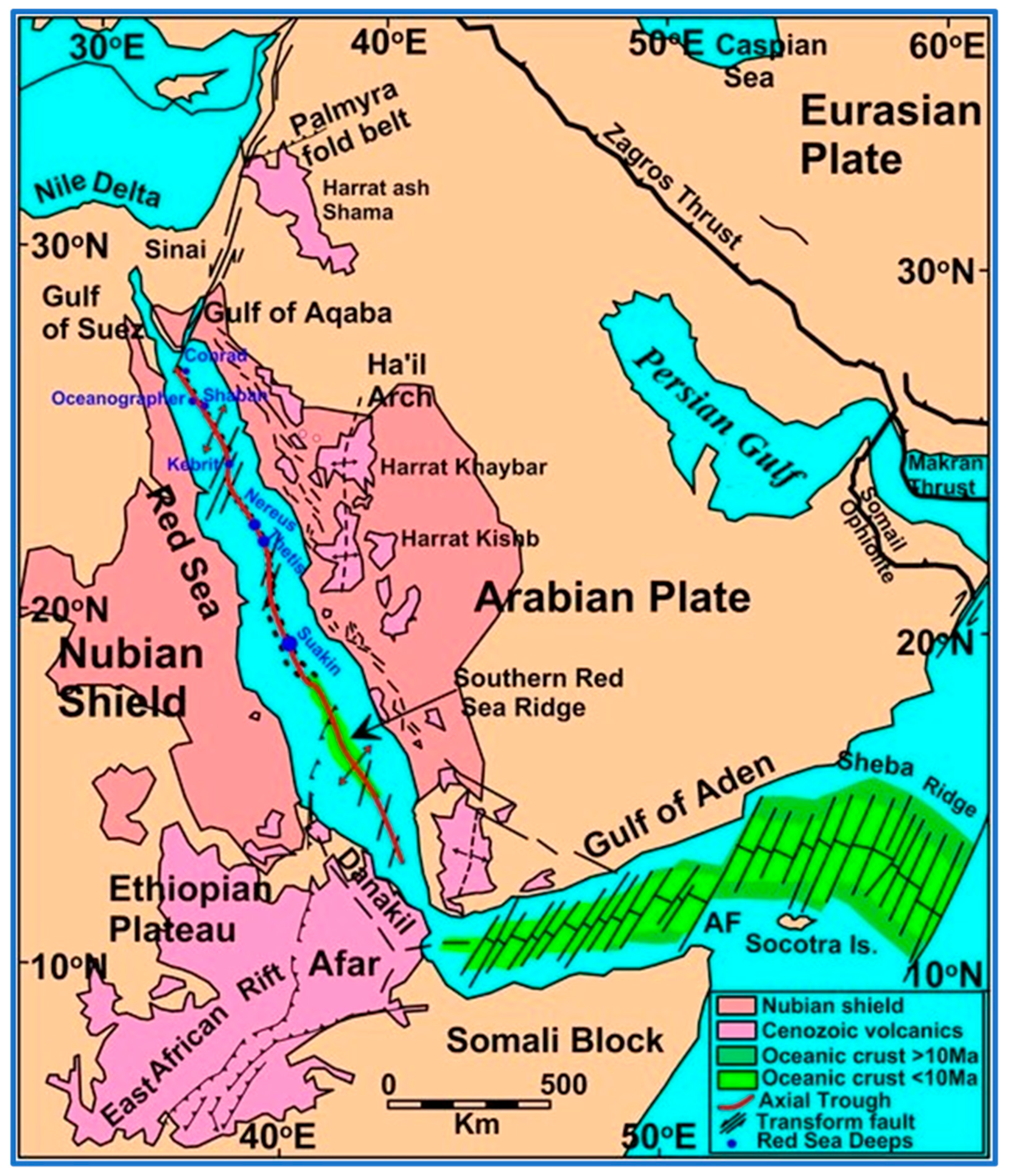
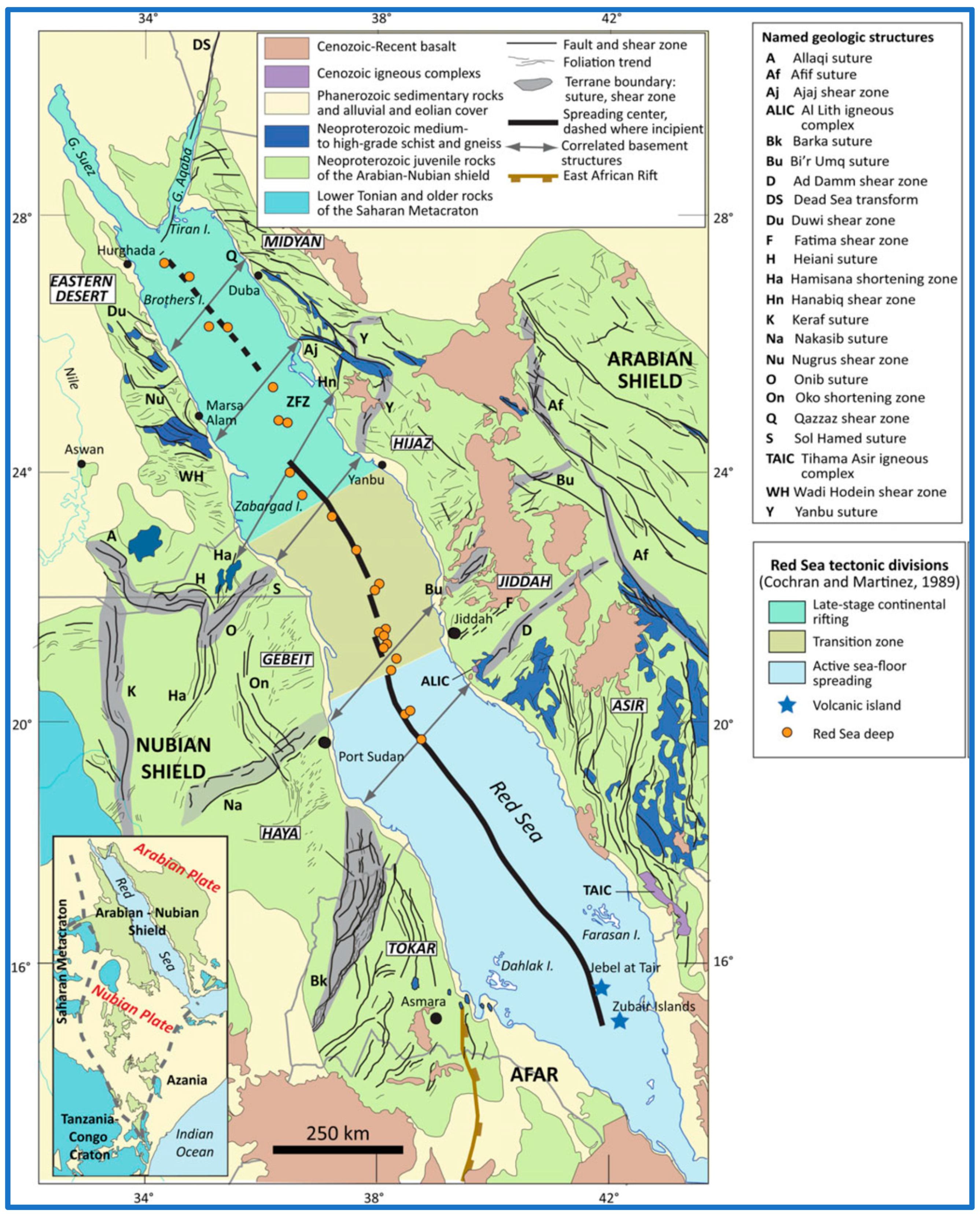
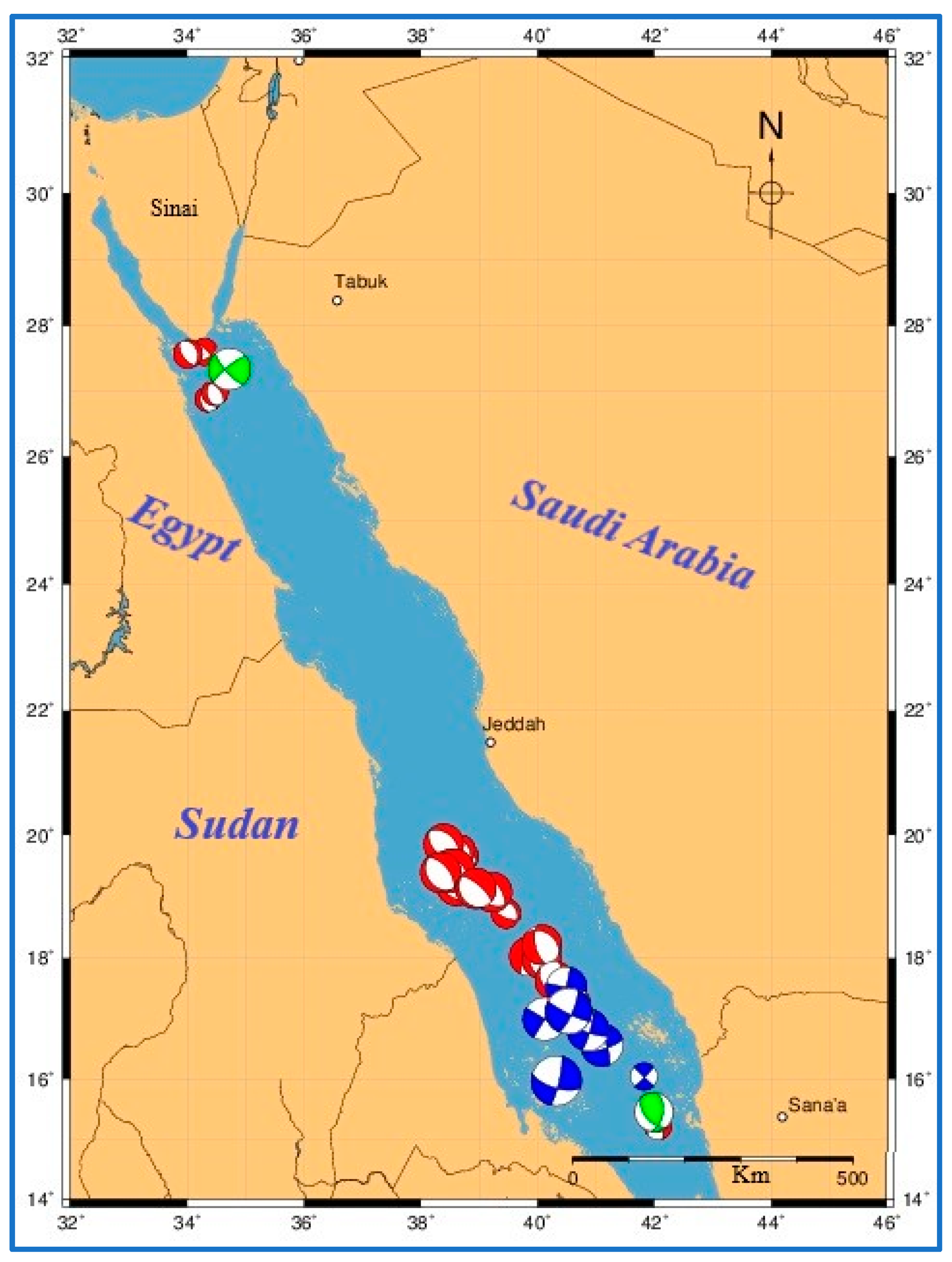
2. Regional Tectonics of the Red Sea

The Red Sea is a long, narrow body of water in the Middle East that links Asia and Africa. The Red Sea is dominated by the divergent boundary between the African and Arabian plates, which actively separates them. The result of this process is the Red Sea Rift (Figure 1), a lengthy dip that runs the length of the Red Sea. Normal and transform faults participate in the intricate fault network that constitutes the Red Sea Rift. Many geological phenomena, including seamounts, volcanoes, and coral reefs, owe their existence to faults that run the length of the rift and create basins and uplifts. The rift has carved out a number of deep oceanic tunnels in the Red Sea, including the Suakin Trough and the central Red Sea Trough. Some of the deepest trenches on Earth can be found here at depths of over 3000 m. Hot springs, geothermal vents, and hydrothermal mineral deposits are abundant in the Red Sea area due to the region’s tectonic activity. As critical habitats for many marine creatures, these characteristics have long been the focus of scientific investigation [1,7].

The Arabian and Nubian (or African) plates presently comprise the Arabian and Nubian (or Red Sea) shields, once part of one continuous mass of Neoproterozoic rocks. The Red Sea is a young ocean around 300 km wide located at the centre of this barrier (Figure 2). The Red Sea is the best example on Earth of an active, developing ocean basin where seafloor spreading has replaced continental rifting [7,8]. According to [8], the Red Sea formed when a piece of Africa broke off and slid into the Arabian Peninsula, creating the East African Rift and the Gulf of Aden Rift. The rifts, which converge at a triple junction in the Afar area of Ethiopia, Djibouti, and Eritrea, exhibit various developmental stages [8].

Observations made using GPS show that the Northern Red Sea is not opening parallel to its boundaries. Instead, according to [11], it is currently broadening in a direction roughly ~0.7 ± 0.1 cm/year parallel to the trend of the Gulf of Aqaba transform boundary. This movement is divided into ~0.15 cm/year of NNW separation across the Suez rift and ~0.44 cm/year of left-lateral shear along the Aqaba transform at the Red Sea–Aqaba–Suez triple junction [11,12]. The E–W extension of about ~0.2 cm/year between Sinai and Arabia [12] adds to this complexity. GPS data have confirmed predicted responses to the earthquakes on the Gulf of Aqaba normal fault. According to [13], the 0.15 cm/year NNW displacement of Sinai, with respect to Africa, can be condensed into 0.14 cm/year of left-lateral shear and the Gulf of Suez Rift’s usual expansion rate of 0.05 cm/year. According to plate tectonic, GPS, and geologic research, the Red Sea is currently enlarging at a rate of 24 ± 1 mm/year in the south and 7 ± 1 mm/year in the north [12]. The authors of [7] stated that the Oligocene–Miocene transition between Eritrea, Egypt, and northwestern Arabia marked the beginning of continental extension, characterised by the intrusion of mafic dikes and normal faulting [9]. Overall, tectonics in the Red Sea is an exciting and dynamic topic that provides insights into the region’s geological past and the processes that are still shaping it today (Figure 1 and Figure 2).

3. Red Sea Seismicity

The continuous tectonic action associated with the Red Sea Rift causes the Red Sea region’s seismic activity. The ongoing activity is largely due to the tectonic plates of Arabia and Africa sliding past one another along the rift. Although most of these activities are on the smaller side, the region has also seen larger tremors. The National Centre for Earthquakes and Volcanoes in Yemen, the Egyptian National Seismological Network, and the Saudi Geological Survey (SGS) continuously keep records of seismic activity in the Red Sea region. These organisations use a system of seismic stations to monitor the region for earthquakes and other seismic activity in real time. Volcanic and seismic activity are both common in the Red Sea area. Volcanic activity has occurred in the area before, and the Red Sea Rift is home to both active and extinct volcanoes. There are other geothermal sites nearby where hot springs and geysers are common. Overall, it is vital to learn about the seismicity of the Red Sea area because it sheds light on the risks associated with earthquakes and volcanic activity, as well as the ongoing geological processes that have shaped the area.

3.1. Historical Seismicity

There has been seismic activity in the Red Sea region for thousands of years, including earthquakes and volcanic eruptions. The Red Sea region has also experienced volcanic activity at various periods. In 1256 AD, a tremendous volcanic explosion on the island of Jabal al-Tair in the Red Sea triggered a massive tsunami that wreaked havoc on the adjacent beaches, becoming one of the most well-known volcanic eruptions in the region. According to the revised historical seismicity, one of the major historical earthquakes in the region hit the city of Medina in modern-day Saudi Arabia in 856 AD. The earthquake caused considerable damage and many deaths. In the past 1400 years, there have been 88 earthquakes between the latitudes of 13° and 30° in the Red Sea region, with magnitudes ranging from 5.6 to 7.0 reported by several researchers, including [14,15,16,17], on the VI to IX intensity scale. Based on their reported damage and/or intensities, only a few earthquakes were assigned magnitudes in this study, all falling within the range of M = 5.6–6. The majority of these historical earthquakes’ epicentres were derived from published sources. The 1196 earthquake that devastated Mecca, Saudi Arabia, and the rest of Egypt was the worst. The epicentre of an earthquake of that magnitude would have been somewhere in the Northern Red Sea area. There were only two quakes of M = 7 on the Richter scale, one in the Northern Red Sea region and the other in the Southern Red Sea region. Although the second epicentre was positioned in the Northern Red Sea region by most researchers, some [18,19,20] located it in the Gulf of Aqaba region, whereas others [15] placed it more than 150 km east of the Gulf of Aqaba.

The Gulf of Aqaba area is considered to be the epicentre of this earthquake based on the published research about inferred ground and archaeological ruptures and deformations [18,19], as well as the fact that it caused a tsunami along the southern coast of Palestine, most likely due to a triggered regional sub-water landslide [21]. One citation specifically mentions one earthquake with a magnitude of 7.4, notably [22]. In actuality, this citation references two earthquakes with magnitude values of 6.2 and 7.4 in the Southern Red Sea region in 1884. Only the 6.2 earthquakes recorded with tsunamis are included in all other references that describe this event. The area around the Red Sea has had several large earthquakes. One of the most notable ones was the 7.5-magnitude Gulf of Aqaba earthquake in 1945, which left extensive devastation in its wake. The Gulf of Suez earthquake in 1984, which had a magnitude of 6.2 and significantly damaged the region’s infrastructure and structures, is another noteworthy earthquake. Overall, the Red Sea region’s past seismicity offers significant insights into the possible dangers brought on by the region’s volcanic activity and earthquakes. It also draws attention to the continuing tectonic processes that affect the area and the need for ongoing observation and study [1].

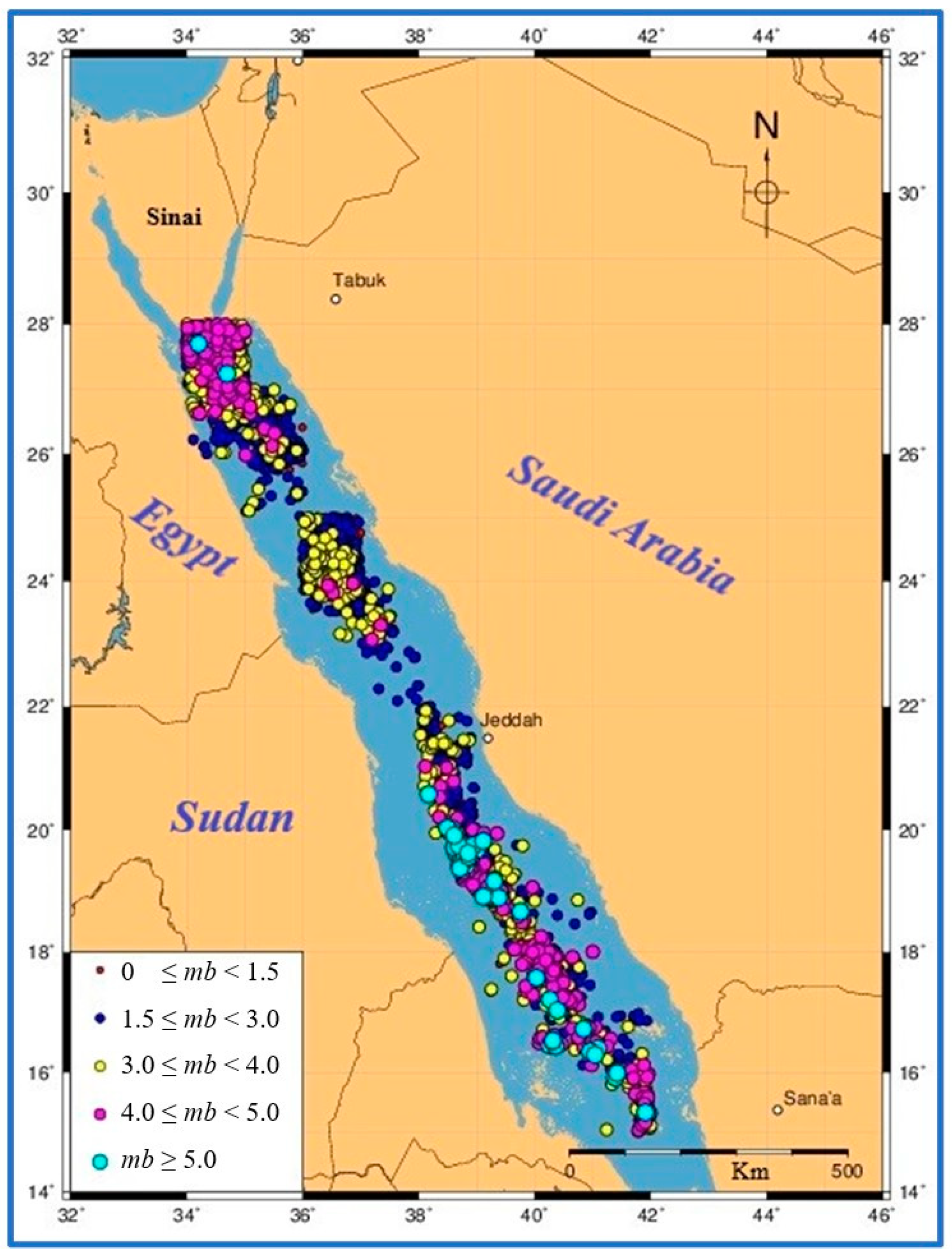
3.2. Instrumental Seismicity

Active tectonics, such as those in the Red Sea region, can be detected and quantified using seismometers. Currently, nearby African and Arabian plates are merging and slowly drifting away from one another at a pace of around 1 cm each year. Close to the Saudi Arabian town of Ba’arin, the region’s biggest earthquake, measuring 7.2 on the Richter scale, occurred in 1993. This earthquake caused widespread damage to local structures and infrastructure. On 28 March 1967, the Red Sea region saw an enormous 6.7-magnitude earthquake. Several moderate earthquakes with magnitudes ranging from 3.0 to 5.0 have occurred in the Red Sea region more recently [23]. Although the local populace frequently feels these earthquakes, they do not inflict much harm. To better understand the tectonic processes occurring there and develop mitigation methods for the risks associated with earthquakes, seismologists and geologists carefully monitor the instrumental seismicity of the Red Sea region.

4. Dataset and Methods

Initially, there were 8077 earthquakes recorded in the Red Sea region, with magnitudes ranging from 0 to 5.7 and focal depths beginning at 0 and ending at 49 km. The International Seismological Centre (ISC) online bulletin [24] compiles this information by integrating phase measurements and data retrieved from local seismological organisations. The earthquake data collection should use comparable magnitude scales to assess the completeness of the earthquake catalogue. Although most events in the research region have been described using the “ml” magnitude scale, only a few events have used the Md, mb, and/or Ms magnitude scales, which were excluded from our study for consistency. Only a few stations collectively recorded 1063 earthquakes with magnitudes less than 1.0, making the majority of their data questionable. Consequently, they were excluded from the data collection to generate a more homogeneous earthquake data catalogue containing 7014 earthquakes with magnitudes of 1.0 ≤ ml ≤ 5.7. To create a time-independent Poisson distribution of seismicity, we applied a declustering process, which specifies earthquakes that occur in clusters, such as foreshocks/aftershocks sequences and swarms, and then removes them from the catalogue.

Several strategies have been used in the declustering procedure, including windowing, deterministic, and stochastic methods [25,26]. Windowing methods are the most widely used deterministic processes. These methods streamline the inventory by considering the region’s geological history and associated seismicity. As a result, it is easier to discriminate between foreshock, mainshock, and aftershock sequences. All dependent events are presumed to occur throughout this window using these methods. Furthermore, they explore a circular geographical window for earthquakes of a larger magnitude, which is inconsistent with fault extension. We included a total of 6527 earthquakes with 1.0 ≤ ml ≤ 5.7 and focal depths ranging from 0 to 49 km in the dataset for the current investigation (Figure 3). Following the use of [26]’s declustering, 487 (6.94%) out of 7014 clustered events were eliminated from the dataset. Out of the 6527 earthquakes chosen, 1793 have a magnitude of 1.0 to 1.5, 3686 have a magnitude of 1.5 to 3, 742 have a magnitude of 3.0 to 4, 290 have a magnitude of 4.0 to 5, and 16 have a magnitude of ≥5.0.

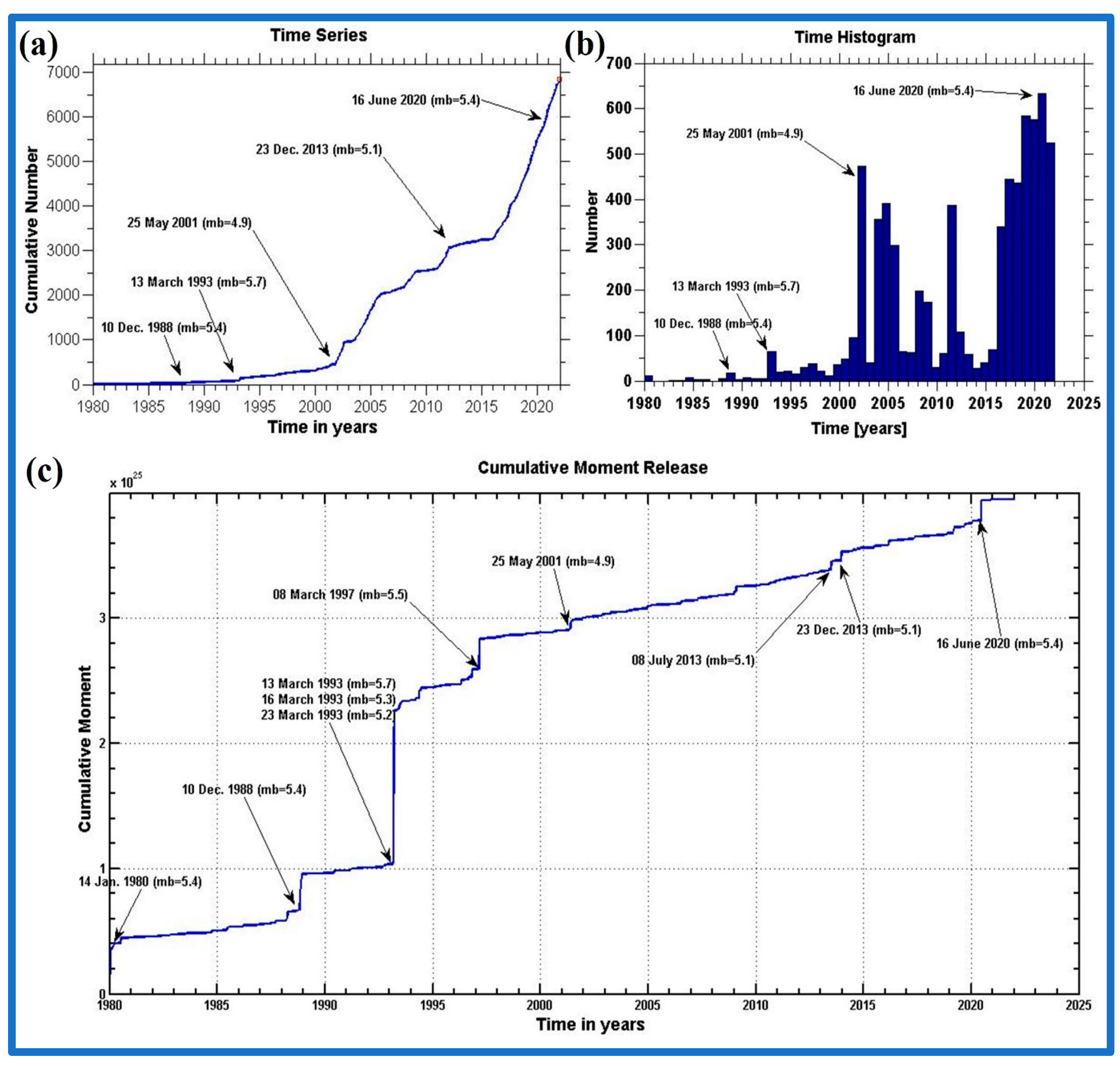
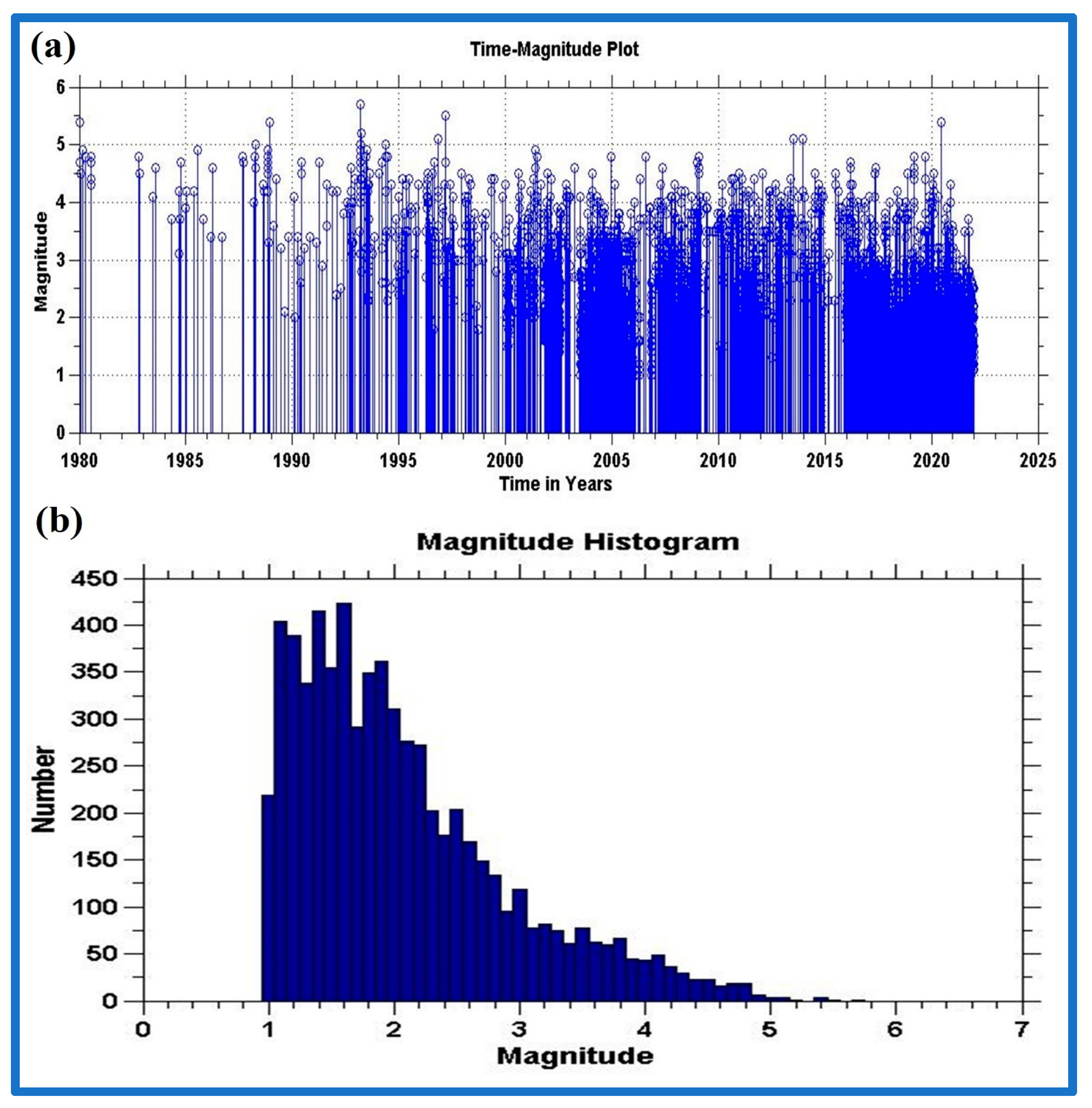
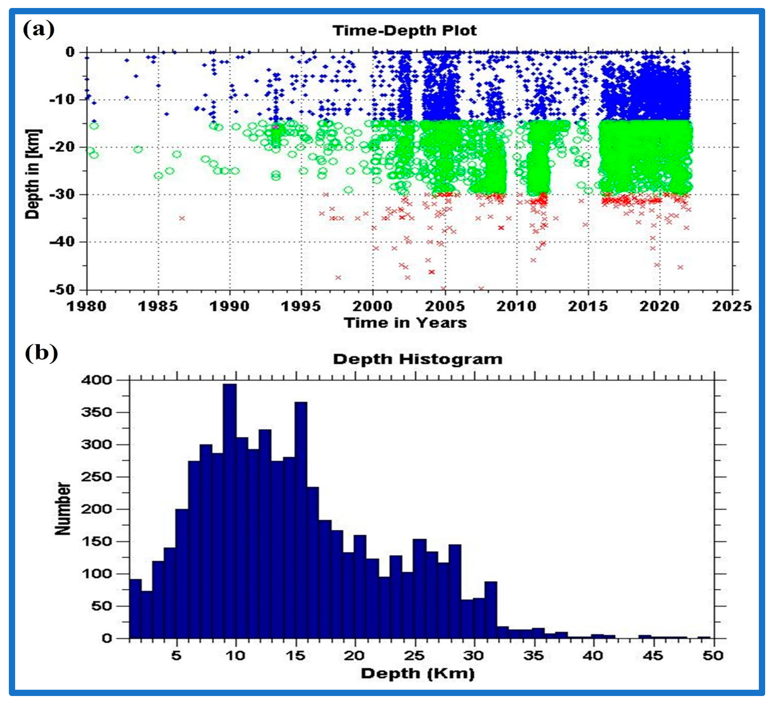
5. Analysis of Earthquake Data

We conducted earthquake data analysis using ZMAP [4]. The time distribution of earthquake measurements (Figure 4) made it clear that there was no network coverage in the Red Sea region. We were advised to start our dataset from 1980 because there were not enough records prior to that year to compare with later data. The evolutions of seismic activity levels from 1980 and 1993 are consistent, with only minor deviations in 1988 after the earthquake on December 10 (mb = 5.4) (Figure 4a–c). Big earthquake sequences with numerous accompanying large aftershocks struck the area in 1993, 1997, and 2001, increasing the cumulative moment number over time. The time histogram and time series charts show a sharp increase in seismic activity after 2001, which may be due to the expansion of the seismic network coverage, the development of data analysis software, and the observation of moderate seismic activity of magnitudes > 5.0. The graph displays earthquakes connected to abrupt shifts in the cumulative moment curve. The 13 March 1993 (mb = 5.7), 25 May 2001 (mb = 4.9), and 16 June 2020 (mb = 5.4) earthquakes are responsible for the greatest modifications.

Figure 5a shows the Red Sea region’s seismic activity across time. Figure 4b displays the magnitude number distribution of earthquakes with ml ≥ 1. Figure 5a shows a considerable rise in earthquake activity in 1993. According to [1], the construction of new seismological stations in Saudi Arabia in the 1990s impacted its ability to identify more moderate earthquakes and, as a result, noticeably greater seismic activity. Beforehand, only significantly moderate and large earthquakes were detected by distant stations, and tiny earthquakes were rarely felt. The magnitude distribution histogram (Figure 5b) demonstrates that most earthquakes had magnitudes between 1.0 and 2.3. Few earthquakes with magnitudes ≥ 5 have been reported, with earthquakes > 3.0 reduced by about 75%. Only a small number of Red Sea earthquakes are recorded at depths > 40 km and up to 50 km, respectively, according to the depth distribution over time and depth histogram (Figure 6a,b). The depth range is between 5 and 16 km.

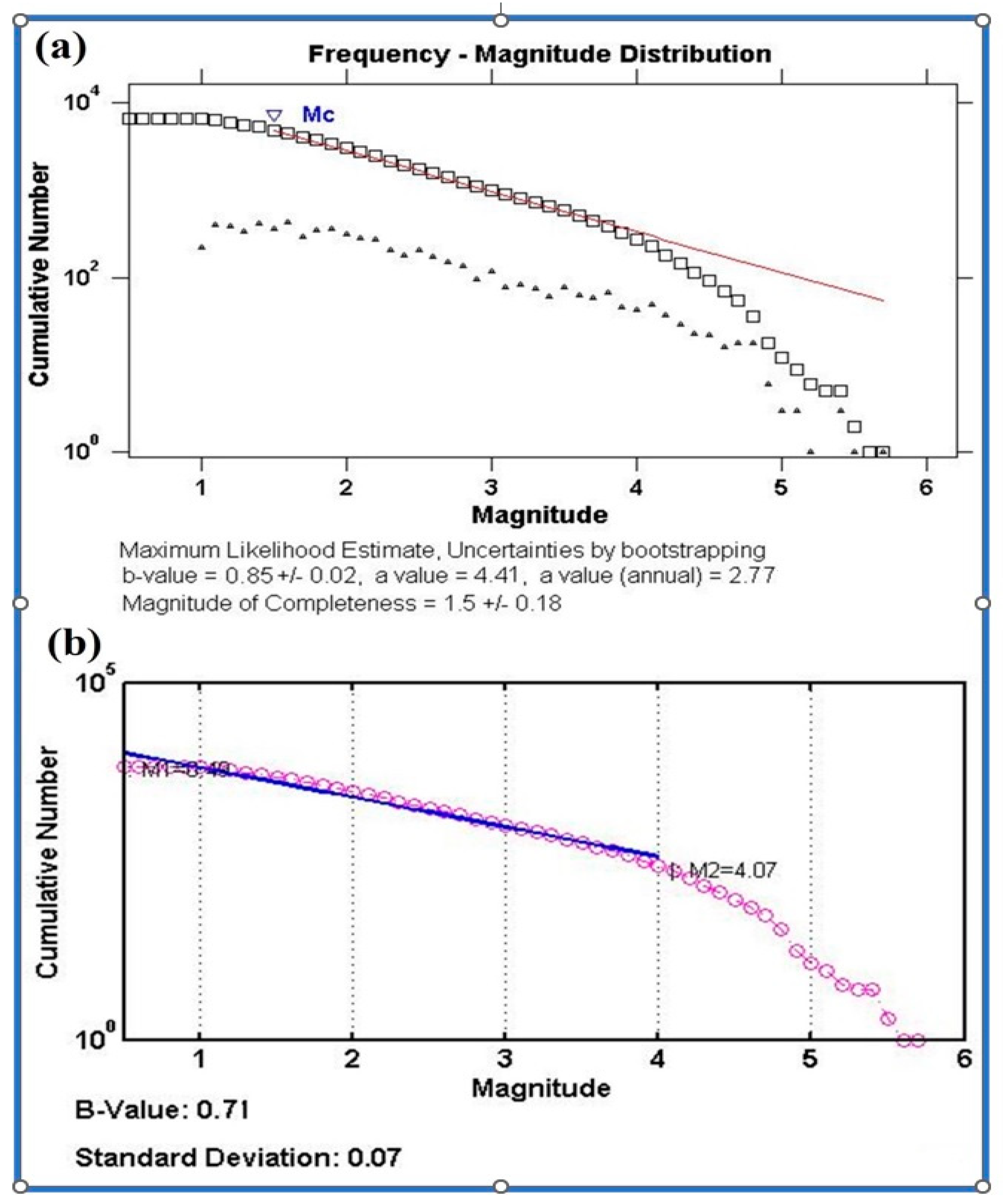
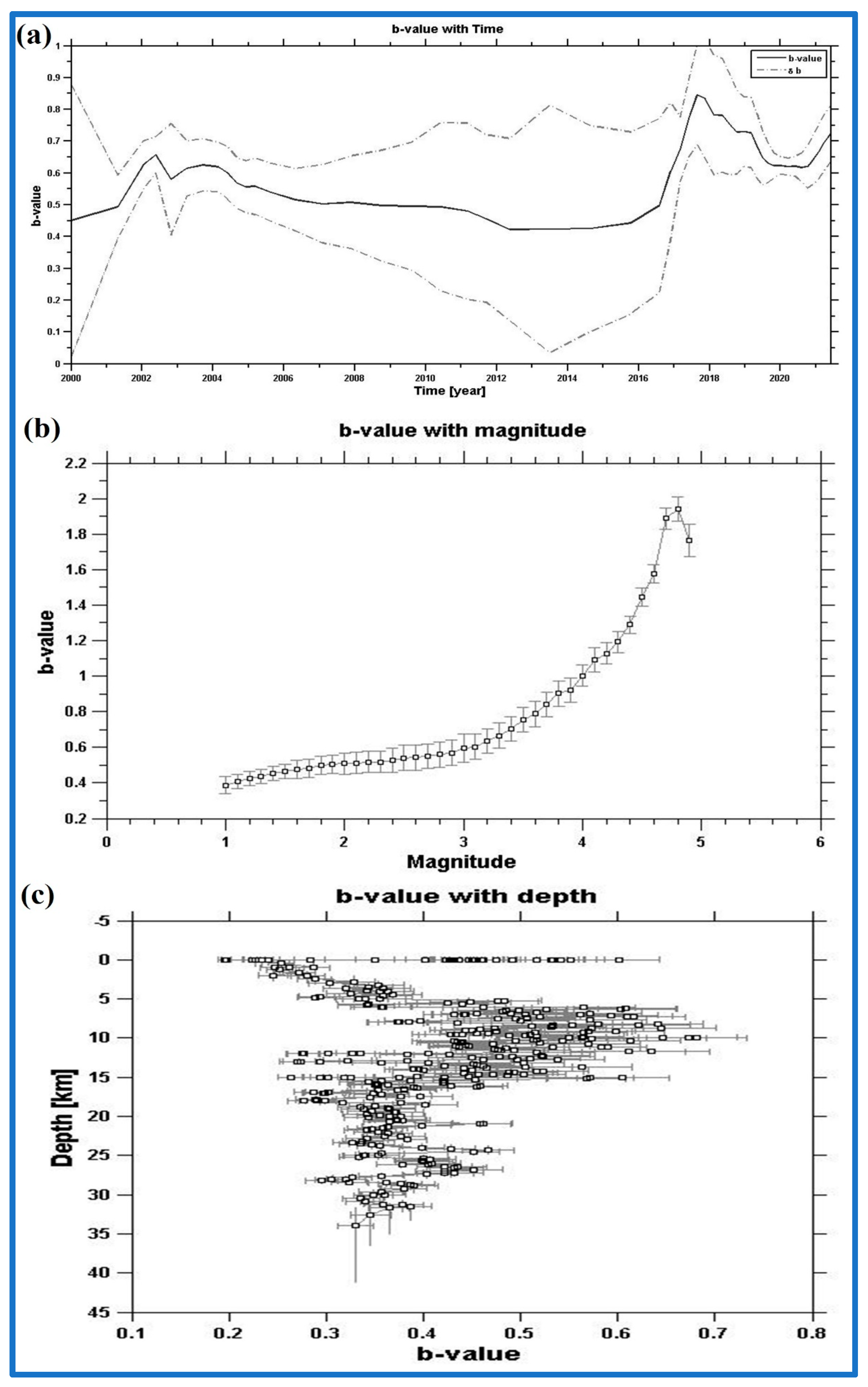
GR Relationship: Mc and b-Value

The authors of [27] proposed the frequency–magnitude distribution (FMD) to relate earthquake magnitude and recurrence time. The following equation shows their relationship:

$$lo{g}_{10} N \left(m\right)=a-bm$$

where N(m) is the number of earthquakes of magnitude m or greater in the selected time period; a and b are positive constants; and m and b are integers. The a-value is a measure of seismic productivity (rate) that varies regionally depending on factors such as territory size, observation period length, earthquake magnitude, and stress levels [28]. The Gutenberg–Richter log-linear proportionality constant is the b-value, which is the slope of the exponential drop of N with increasing magnitude events in earthquake data collection. The authors of [29,30] found that the b-value is inversely related to stress, ductility, rock type, and stress and strain distribution. A b-value near one is typical of tectonically active regions [31]. b-value examinations determine whether the size distribution, stress, and faulting types of earthquakes have obvious and/or direct relationships. The characteristics of the Earth’s crust and physics can also be deduced from the b-value. Another definition of Mc is the magnitude at which a seismic network provides complete event detection, meaning that no events are missed [32]. In other words, it is the smallest magnitude at which each earthquake in a space–time volume is successfully identified [33,34,35,36].

Due to its computing speed, the maximum curvature approach is currently the more used Mc estimate method. The point of maximum curvature is determined by the highest value of the first derivative of the earthquake curve’s frequency–magnitude curve as a magnitude of completeness [37,38]. The magnitude bin in the non-cumulative FMD with the highest frequency of events matches this method (triangle symbols in Figure 7a). Using the Monte Carlo approximation of the bootstrap method, uncertainties are also considered [39]. The results of an algorithmic estimation are Mc = 1.5 ± 0.18, b = 0.75 ± 0.02, and a = 4.37. The endpoint at the flat line displays the appropriate a-values (4.07) and b-values (0.71) with a standard deviation of 0.07 when employing the relevant manual curvature assumption and connecting the lowest and maximum magnitudes (M1 and M2) (Figure 7b).

We examined the b-values versus time graph for the entire region to determine changes in b-values over time. To analyse the dynamics of b-values across time, the ZMAP program uses the sliding time window method. The size of the window is determined by how many events are in the catalogue. Seven hundred events were randomly chosen from the sample window. The results are shown in Figure 8a. For the large earthquakes in the database, the image depicts multiple rapid shifts in the b-value over time. Stress fluctuations caused by significant occurrences in the Red Sea region are responsible for the plots’ high-frequency oscillations. The remarkably flat curve from 2004 to 2016 suggests that the network setup and recording processes have not altered. At the start of the plot, the b-value had an average between 0.4 and 0.65. We also observed a smooth plot around 0.5 before and after 2016. The b-value increased significantly between 2016 and 2018 (0.5 to 0.85) before declining to an average of 0.70 at the conclusion of the plot (Figure 8a).

Figure 7. (a) Frequency–magnitude distribution calculated by the maximum curvature technique. Mc is the cut-off magnitude. Squares and triangles show the cumulative earthquakes for each magnitude value as well as the earthquake numbers, respectively. (b) The frequency–magnitude distribution using the corresponding manual curvature assumption between M1 and M2. The endpoint on the flat line shows the corresponding a and b-values.

Figure 7. (a) Frequency–magnitude distribution calculated by the maximum curvature technique. Mc is the cut-off magnitude. Squares and triangles show the cumulative earthquakes for each magnitude value as well as the earthquake numbers, respectively. (b) The frequency–magnitude distribution using the corresponding manual curvature assumption between M1 and M2. The endpoint on the flat line shows the corresponding a and b-values.

After choosing the portion of an earthquake catalogue that is relatively homogeneous in location, time, and magnitude band, ZMAP offers the option of mapping the b-value with magnitude and depth assuming that the b-value is essentially constant across time. As a function of space, first-order variations are anticipated. Indicating that the completeness magnitude is ~3.0, the b-values stabilise above the cut-off magnitude value of ~3. A gradual increase in b-values may result from the frequent occurrence of moderate earthquake sizes over the completeness magnitude and up to ml = ~4.8. An overturning slope can be caused by less frequent but stronger earthquakes (magnitude ≥ 5.0) (Figure 8b). Figure 8c shows how the b-values change as the depth of the earthquake increases. The prevalence of earthquakes in various magnitude bins, particularly at depths between 5 and 15 km, indicates a higher b-value distribution. This frequency might be due to the uniformity of the crustal media and the high static pressure of the surrounding rock. Furthermore, early ruptures are more likely to become big ruptures, causing large-magnitude earthquakes more frequently. The observed changes in the b-value with depth, particularly between 0 and 15 km, where large-magnitude earthquakes were most common, may be due to variations in the ratio of weak to strong earthquakes or an increase in crustal material strength due to rising temperatures and confining pressure.

Figure 8. The variations of b-value with (a) time; (b) magnitude; (c) depth.

Figure 8. The variations of b-value with (a) time; (b) magnitude; (c) depth.

After 2018, dense station deployments in the study area could detect most earthquakes with magnitudes of ≥1.2 and led to smaller Mc values ≥ 1.1 (Figure 9). In 2020, events with magnitudes of ≤0.5 were densely recorded and may change seismicity parameter values in a few years once more data have been gathered. However, the Mc variants are consistent with the odd behaviour of the Mc vs. time plot.

6. Fractal Dimension

Earthquake clustering is a fundamental feature of Earth’s seismicity that holds true across all scales of observation. Thus, geographical and temporal distributions of earthquakes are believed to be a scale-invariant phenomenon. Fractal dimensions can be used to describe scale-invariant phenomena since they are governed by fractal statistics. Numerous researchers, including [40,41,42,43,44,45], claim that the spatial distribution of earthquake epicentres is fractal. The distribution of earthquake epicentres can be characterised by the correlation dimension [40,46,47], which measures the spacing or clustering of features in a set of sites.

The complexity or irregularity of earthquakes’ spatial distribution within a specific region is measured using the earthquake fractal dimension, sometimes denoted as $Dc$. It is based on the concept of fractals, which are mathematical sets exhibiting self-similarity at different scales. It should be noted that the earthquake fractal dimension is a statistical measure that might change based on the scale and resolution of the analysis. Various locations and fault systems may exhibit different fractal dimensions representing their unique tectonic and geological properties. Other variables, including the accuracy and completeness of the data, can also impact the computed fractal dimensions. The two-point correlation dimension ($Dc$) is a useful tool for determining fractal size. The fractal dimension Dc and the correlation function C(r) were first linked by [6]:

$$C\left(r\right)=\frac{2\mathrm{N}\left(\mathrm{R}<\mathrm{r}\right)}{\mathrm{N}\left(\mathrm{N}-1\right)}$$

$$Dc=\lim [\frac{\log C\left(r\right)}{\log r}]$$

where r denotes the separation between two epicentres and N denotes the number of event pairs separated by a distance of R < r. The following formula is used to compute the distance r between two epicentres:

$$\mathrm{r}=co{s}^{-1} (\cos \mathsf{\theta }\mathrm{i}\cos \mathsf{\theta }\mathrm{j}+\sin \mathsf{\theta }\mathrm{i}\sin \mathsf{\theta }\mathrm{j}\cos \left(\varnothing i-\varnothing j\right))$$

where $\left(\mathsf{\theta }\mathrm{i},\varnothing i\right)$ and $\left(\mathsf{\theta }\mathrm{j},\varnothing j\right)$ represent the latitudes and longitudes of the ith and jth events, respectively. On a double logarithmic plot, the slope of the (r) graph against r can be used to determine the fractal dimension value ($Dc$).

When the locations of the earthquake epicentres are too close, the fractal dimension is smaller than when they are farther apart [48]. Seismic heterogeneity in a fault system can be measured using the fractal dimension, which is affected by the stress field and local geological and structural heterogeneity [49]. Therefore, changes in the fractal dimension’s values can be interpreted as a quantitative indicator of local stress heterogeneity’s evolution. When $Dc$ is high, seismic activity is spread out over a wide area. When $Dc$ is low, activity is clustered in a small area. Fractal dimensions can help locate unbroken locations or seismic gaps that will eventually rupture.

We determined the earthquake fractal dimension in this work by evaluating the statistical features of earthquake locations, such as epicentres and hypocentres. We used the box-counting methodology to determine $Dc$, which is a popular method. The study area was divided into a grid of smaller boxes in this manner, and the number of boxes containing at least one earthquake was counted for different box sizes. We observed a linear relationship after plotting the logarithm of the box size against the logarithm of the number of boxes, and the slope of this line corresponds to the fractal dimension. We calculated the fractal dimension of the Red Sea region using 6856 earthquakes. The results show a rather high fractal dimension ($Dc$ = 2.3), which is significant due to the Red Sea’s geological complexity and structural diversity (Figure 10). This finding demonstrates the erratic spread of earthquakes. The low b-value and comparatively high $Dc$ resulted from major earthquakes that happened in the past and the increased stress they caused.

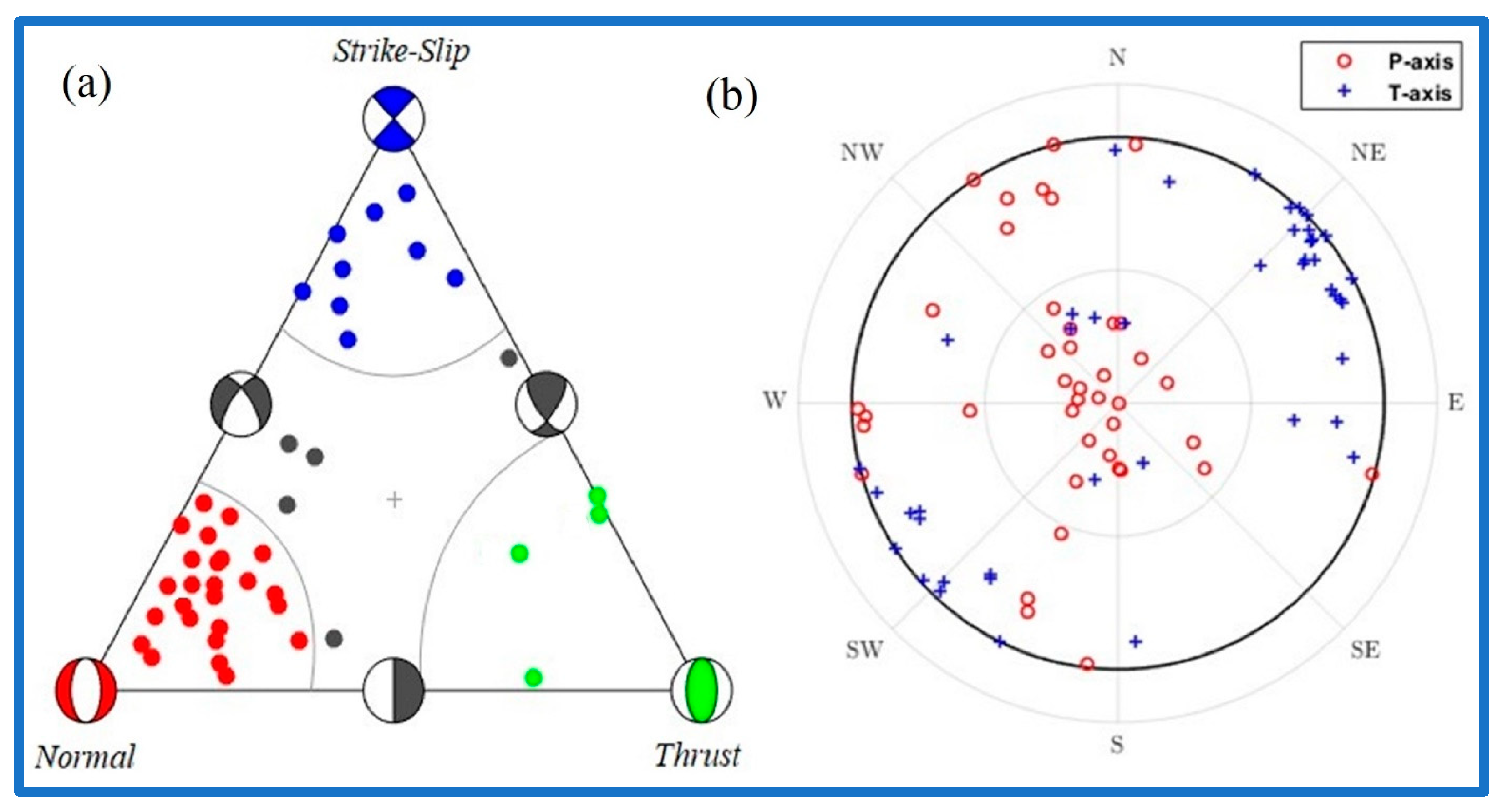
7. Focal Mechanisms and Stress Analyses

Focal mechanism solutions (FMSs) define the geometry and mechanics of faulting during earthquakes. An earthquake’s waveforms can be used to generate FMSs, as these waves propagate in all directions and are recorded by several seismograms located at varying distances and azimuths from the epicentre. Since the waveforms’ radiation patterns are geometry-dependent, knowing the fault geometry is crucial to finding the focal mechanism’s response [50,51]. Various ongoing tectonic research initiatives use FMSs to invert stress tensors, assign tectonic regimes, orient maximum horizontal stresses, conduct seismotectonic analyses, and so on.

We compiled a total of 44 focal mechanism solutions from the ISC database for this investigation (Figure 11). The gathered events all had magnitudes greater than 4.0. Most of the events occurred in the upper 40 km of the crust. These processes are compatible with the general perception of movement along these faults, and their distribution over the region relates to active fault locations in the area. Since the region is characterised by extensional tectonics, the area is dominated by normal fault solutions. The strike-slip components in certain normal solutions are negligible, whereas they are quite large in others. Most of the solutions for the Northern Red Sea area exhibit normal fault mechanisms with minor to no strike-slip components. However, a few solutions indicate predominantly strike-slip components. The Southern Red Sea area exhibits both normal and strike-slip FMSs due to its complicated tectonic nature. Few oblique slip solutions have been documented in the Northern and Southern Red Sea regions.

7.1. Michael’s Stress Tensor Analysis

Numerous methods have been suggested to extract the tectonic stress orientation and stress ratio (R) from earthquake focal mechanisms [52]. The authors of [5] used a linear least-squares inversion technique to determine the stress tensor. Using this technique, they could determine the directions of the three main stress axes and identify the stress tensor that best matched previously published focal processes [53]. The fault plane did not need to be defined for this linear inversion technique. By contrast, this approach uses bootstrap resampling to randomly select a fault plane from a set of nodal planes. Variance, which is the angle between each unique focal mechanism and the assumed tensor, can be used to quantify a stress field’s heterogeneity [54]. For a stress field to be spatially uniform, the variance value must be <0.2. According to [54], larger values represent stress orientations that do not match well, keeping the stress field heterogeneous within the investigated volume. According to the hypotheses of [55,56], the seismic slide follows the direction of the strongest shear stress.

Depending on the fault orientation and intensity, a single solution’s pressure and tension axes can differ from the principal stress directions [57]. The focal mechanism’s dilatational quadrant can have any orientation for maximal compressive stress. Therefore, weakly limited primary stresses result from single-focused mechanisms or from numerous processes with comparable orientations. However, several solutions with varying orientations inside a constant stress zone can help identify principal stress directions. In this study, we used the linearised stress inversion technique developed by [5] and ran it through ZMAP [4]. We inverted the research area’s stress tensor using Michael’s approach and FMSs (Figure 12). Figure 12a,b shows that the largest principal stress (σ1) is vertical, the minimal stress axes (σ3) are sub-horizontal, the intermediate principal stress (σ2) trends NE–SW, and the highest principal stress (σ1) is vertical. In the region that characterises the homogeneity of stress orientations, the variance, which should not be >0.2, is 0.19. The faulting pattern in the area is normal, as indicated by the Phi ratio of 0.76, also known as the stress ratio (R) (Figure 12a,b). Since FMSs represent higher moderate-sized earthquakes (mb ≥ 4) centred on the Southern Red Sea, the stress inversion was repeated only in this source zone. According to the inversion results for the southern part of the Red Sea, the results are almost the same. Michael’s strategy did not work in the Northern Red Sea, which has fewer focal mechanism solutions. Therefore, the southern section may significantly influence the stress regime of the Red Sea region (Figure 12c,d).

7.2. Distributions of Pressure and Tension (P-T) Axes and Rake

The triangle diagram was developed by [2] as a new graphical technique to describe and comprehend the typically anisotropic in situ stress states detected in rocks. The method displays three-valued stress states in two-dimensional space by mapping three-dimensional stress space onto a triangular-coordinate (ternary) diagram and plotting the measured stress states as points [2]. The ternary technique for visualising focal mechanisms by [3] employs each vertex to represent normal, thrust, and strike-slip focal mechanisms. Ternary diagrams illustrate the three ‘pure’ strike-slip, normal, and thrust mechanisms at an earthquake’s three vertices [42,58]. According to [3], triangle diagrams represent focal processes quantitatively using the dip angles of the T, B, and P axes. They showed how to use quantitative methods for displaying the focal mechanism orientations of earthquake groups on a triangle diagram [59]. The seismic zones are separated into four segments in the ternary figure: thrust, strike-slip, normal areas, and ‘others’, which contains all the other mechanisms.

Most earthquakes in the Red Sea region have normal solutions, as shown by the rake-based ternary diagram in Figure 13a, which is compatible with the movement of the research area and the Red Sea region’s extensional regime. In addition to normal faults, the research region also has several strike-slip faults, which are primarily located in the southern section. The northern and southern sections of the Red Sea area also have thrust solutions. The pressure and tension (P-T) axes (Figure 13b), which represent the focal mechanism solutions of the largest earthquakes in the Red Sea region, show a NW-SE compression axis and an NE–SW tension axis.

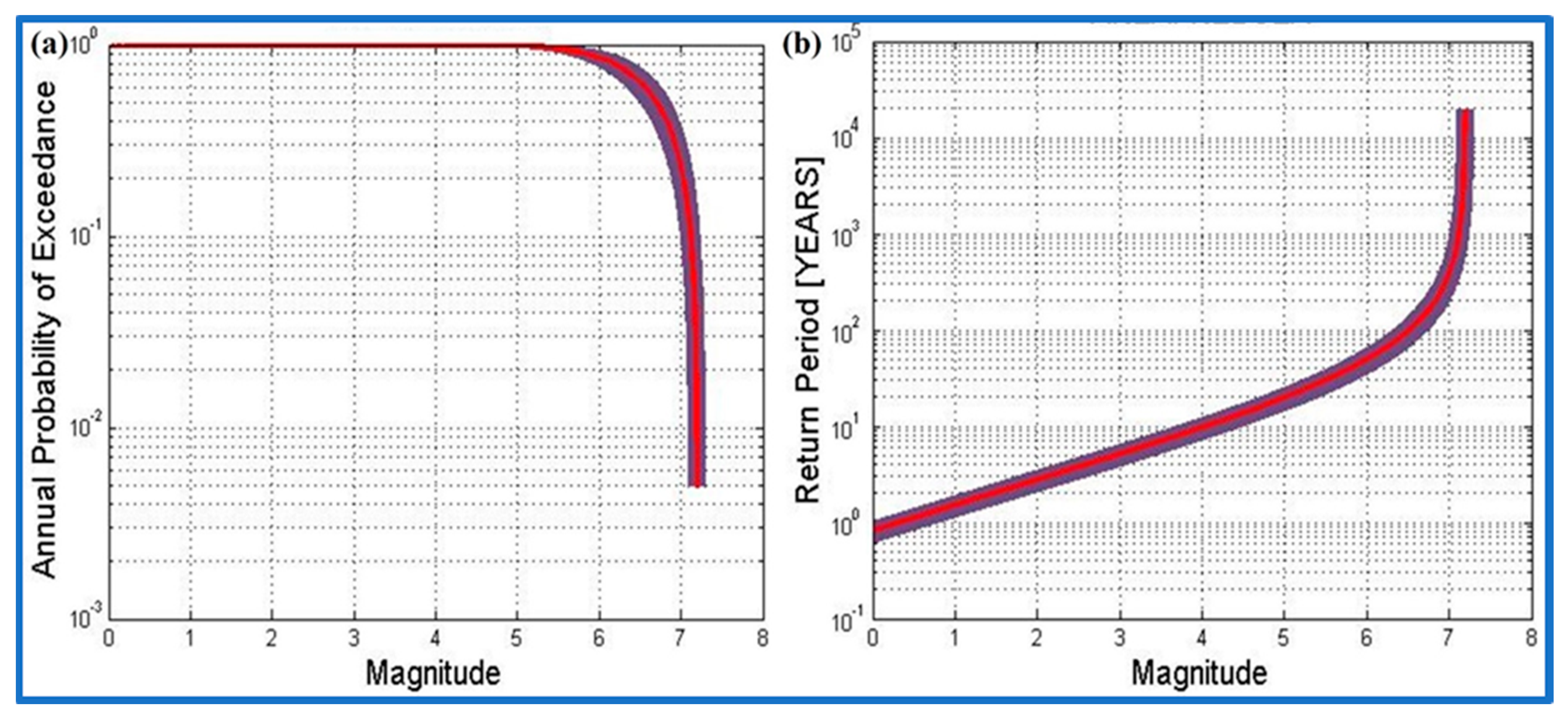
8. Probabilities of Earthquakes and Return Periods

The G-R relation of earthquake frequency magnitude distribution [27] and the study of annual extreme values [60,61] are the two most popular methods for calculating earthquake hazard parameters. Both methods calculate Red Sea earthquake frequencies and return periods. The equations in [6] predict fractal dimension values (Dc), which reveal seismic activity heterogeneity. The spatial variation of the a- and b-value parameters, as well as the neotectonic features, all contribute to a region’s total seismic hazard rating.

Using the obtained a- and b-values from the Gutenberg–Richter relation, the frequency with which earthquakes of varying magnitudes occur in a given region can be determined. Most earthquake prediction models employ the Poisson model. This model assumes that the location, time, and magnitude of each earthquake in a region are unrelated to one another. Thus, the following equation can forecast earthquake risk in a given area:

$$P \left(M\right)=1-e^{-N\left(M\right)*T}$$

where N(M) is the annual mean number of earthquakes that occur in a region with a magnitude greater than or equal to M over a specified time period $T$.

N(M) is determined using the equation below and derives from the Gutenberg–Richer relation:

$$N\left(M\right)={10}^{a-bM-\log Tobs}$$

where Tobs is the observation interval for each region, and a and b are from the Gutenberg–Richter relation’s frequency magnitude distribution. The following equation calculates the earthquake return period:

$$Tm=\frac{1}{N\left(M\right)}$$

Regression models estimate the size. The authors of [62] found a link between rupture magnitude and average surface displacement using historical and current data. Data from all faults determined the magnitude (M) and surface rupture length (L).

Short-term instrument data and historical earthquake observations can determine seismic hazard parameters. Data catalogues are an additional tactic, but due to limited observation time and high error rates, they are less effective [63]. The authors of [64] developed a method that uses mixed data, including powerful historical and instrumental earthquakes, in addition to catalogue data above a specific magnitude threshold. In this method, models of earthquake occurrence are represented by Bayesian Poisson–Gamma distributions and Bayesian Exponential–Gamma distributions in time and earthquake magnitude, respectively. These models help incorporate the uncertainty brought on by erratic temporal seismicity.

We used HA2, a MATLAB-based computer code [64], to determine the seismic hazard parameter in the current investigation. We performed a seismic hazard assessment using HA2, which considers both the temporal fluctuation of seismicity and the incompleteness of the seismic catalogues. To estimate the strong magnitude occurrences in the research area, we combined 7283 earthquakes collected by the ISC along with recent instrumental activity recorded by various global networks since 1962. The authors of [65] analysed maximum magnitude data using used Gumbel’s Type I extreme event statistics. Our findings help quantify the risks from earthquakes in the area in terms of their occurrence probabilities. Figure 14a and

Table 1. Return periods and annual probability of exceedance for certain earthquake magnitudes.

Magnitude	Return Period	Probability of Exceedance (Years)
		1	10	50	100
4	9.70 × 100	0.99965	1	1	1
4.1	1.04 × 101	0.99947	1	1	1
4.2	1.11 × 101	0.99922	1	1	1
4.3	1.19 × 101	0.99885	1	1	1
4.4	1.27 × 101	0.99834	1	1	1
4.5	1.36 × 101	0.99762	1	1	1
4.6	1.46 × 101	0.99662	1	1	1
4.7	1.57 × 101	0.99527	1	1	1
4.8	1.69 × 101	0.99346	1	1	1
4.9	1.82 × 101	0.99104	1	1	1
5	1.97 × 101	0.98787	1	1	1
5.1	2.13 × 101	0.98375	1	1	1
5.2	2.31 × 101	0.97845	1	1	1
5.3	2.50 × 101	0.97172	1	1	1
5.4	2.73 × 101	0.96325	1	1	1
5.5	2.97 × 101	0.95271	1	1	1
5.6	3.26 × 101	0.93971	1	1	1
5.7	3.58 × 101	0.92384	1	1	1
5.8	3.95 × 101	0.90466	1	1	1
5.9	4.38 × 101	0.88166	1	1	1
6	4.88 × 101	0.85436	1	1	1
6.1	5.48 × 101	0.8222	0.99999	1	1
6.2	6.20 × 101	0.78466	0.99999	1	1
6.3	7.09 × 101	0.74117	0.99996	1	1
6.4	8.20 × 101	0.6912	0.99988	1	1
6.5	9.63 × 101	0.63419	0.99966	1	1
6.6	1.16 × 102	0.56965	0.99901	1	1
6.7	1.42 × 102	0.49708	0.99704	1	1
6.8	1.83 × 102	0.41603	0.99095	1	1
6.9	2.50 × 102	0.32611	0.97176	1	1
7	3.85 × 102	0.22698	0.90975	0.99993	1
7.1	7.91 × 102	0.11835	0.70391	0.99515	0.99991

show earthquake probabilities occurring in the study area over 10-, 50-, and 100-year return periods. The probability curve illustrates the decreasing possibility of a magnitude-related earthquake occurring at 10, 50, and 100-year return intervals. We used the data to reliably predict when earthquakes of varying magnitudes would occur in the study area (Figure 14b and Table 1).

9. Discussion and Conclusions

The frequency–magnitude analysis of the historical data, according to [1], shows that the b-value is 1.17. When instrumental events with magnitudes >5.6 were considered, the b-value reduced considerably to 0.85. The authors of [66] divided the Red Sea into three distinct seismogenic source zones (Southern Red Sea, Central Red Sea, and Northern Red Sea) and obtained b-values of 1.0, 0.91, and 1.13, respectively. We determined a slight decrease of about 10% in our results from the study by [66], which is reasonable considering the Red Sea as a one-source zone and the amount of data we used.

The authors of [66] indicated that the numbers of earthquakes per year with a magnitude of 5 in the three Red Sea seismic zones are 0.043, 0.038, and 0.047, respectively (i.e., such earthquakes occur at a frequency of 23, 26, and 21 years, respectively). According to this study’s frequency–magnitude results, the overall average recurrence periods for magnitudes 5, 6.0, and 7.0 were 20, 49, and 385 years, respectively, which agrees with the previous study in the same region.

According to the instrumental data’s frequency–magnitude analysis, the threshold magnitude in the current study was 1.5. The b-value, which represents regional stress situations and associated energy release modalities, had a value of 0.85, less than that seen in historical data, and averaged between 0.4 and 0.85 over time, indicating modest stress accumulation. We used the stress-related b-value variation resulting from the frequency–magnitude relationship to differentiate between stress and crustal heterogeneity. Low b-values have been linked by [29,67] to times of elevated shear stress or effective stress. Increased heterogeneity or crack density in the rock mass causes high b-values [68], but the presence of resistant blocks (asperities) in the rocks causes b-values to decrease. Most earthquakes with reported b-values up to 0.75 occurred at shallow depths (between 5 and 15 km). Considerably low b-values delineate the accumulation of seismic energy at depths below 5 km. The Red Sea region’s low b-value indicates an increased probability of greater magnitude earthquakes, which is consistent with [69]. After 2019, the trend in Mc will determine the sum total of information for all earthquakes > 1.1 on the Richter scale.

The earthquake fractal dimension provides insights into the earthquakes’ spatial organisation and clustering within a region. A larger fractal dimension (nearly 2) denotes a more complex and regular distribution of earthquakes that either occur in clusters or along fault lines. On the other hand, a lower fractal dimension (nearly 1) suggests a more uniform and random distribution of earthquakes. Bottom of Form.

Using 6856 earthquakes, we determined the fractal dimension of the Red Sea region, which showed a relatively high fractal dimension ($Dc$ = 2.3) due to its geological complexity and structural diversity. This value indicates the regular distribution of earthquakes, which occur in clusters or along fault lines. Larger earthquakes in the past increased stress levels, resulting in low b-values and relatively high DCs in the Red Sea region.

Fault plane solutions reveal that major Red Sea earthquakes have normal solutions matching the region’s extensional regime and motion. Strike-slip faults are quite common in the region, especially in the Southern Red Sea. Some thrust solutions can also be found in the northern and southern parts of the Red Sea area. The pressure (P) and tension (T) axes are observed to run from NW to SE, and NE to SW, respectively. The stress inversion shows that the maximum principal stress axes (σ1) are oriented in the vertical direction. The axes of least stress (σ3) are subhorizontal and strike NW–SE, whereas the intermediate principal stress axes (σ2) trend NE–SW. The variance defining the stress direction homogeneity in the area, which should not be more than 0.2, was assessed. Our results show that the variance was 0.19, which is acceptable. The stress ratio (R = 0.76) classifies the faulting type and suggests normal faulting, which is common in the region.

The rigorous analyses undertaken to assess the statistical patterns of large earthquake occurrences in the studied area generated interesting results. The annual probabilities of earthquake activities at various magnitude levels are comparatively <1 for mL ≥ 6 events. The return periods for earthquakes with magnitudes of 4.1 ≤ mL ≤ 5.0 are estimated to be between 10 and 20 years and between 20 and 50 years for earthquakes with magnitudes of 5.0 ≤ mL ≤ 6.0. In addition, we determined that the return periods for earthquakes with magnitudes of 6.0 ≤ mL ≤ 7.1 range from 50 to 800 years (Table 1, Figure 14b). These findings indicate that smaller earthquake magnitude levels occur more frequently than larger ones. Furthermore, for earthquakes with mL = 5.0, 6.0, and 7.0, the recurrence intervals are ~20, ~49, and ~385 years, respectively.

References

1. El-Isa, Z.H. Seismicity and seismotectonics of the Red Sea Region. Arab. J. Geosci. 2015, 8, 8505–8525. [Google Scholar] [CrossRef]
2. Swolfs, H.S. The Triangular Stress Diagram a Graphical Representation of Crustal Stress Measurements; Geological Survey Professional Paper, 1291; United States Government Printing Office: Washington, DC, USA, 1984; p. 19. [Google Scholar]
3. Fröhlich, C. Triangle diagrams: Ternary graphs to display similarity and diversity of earthquake focal mechanisms. Phys. Earth Planet. Inter. 1992, 75, 193–198. [Google Scholar] [CrossRef]
4. Wiemer, S. A software package to analyze seismicity: ZMAP. Seismol. Res. Lett. 2001, 72, 373–382. [Google Scholar] [CrossRef]
5. Michael, A. Use of focal mechanisms to determine stress: A control study. J. Geophys. Res. 1987, 92, 357–369. [Google Scholar] [CrossRef]
6. Grassberger, P.; Procaccia, I. Measuring the strangeness of strange attractors. Phys. D 1983, 9, 189–208. [Google Scholar] [CrossRef]
7. Bosworth, W.; Huchon, P.; McClay, K. The Red Sea and Gulf of Aden basins. J. Afr. Earth Sci. 2005, 43, 334–378. [Google Scholar] [CrossRef]
8. Bonatti, E. Punctiform initiation of seafloor spreading in the Red Sea during the transition from a continental to an oceanic rift. Nature 1985, 316, 33–37. [Google Scholar] [CrossRef]
9. Stern, R.J.; Johnson, P.J. Constraining the Opening of the Red Sea: Evidence from the Neoproterozoic Margins and Cenozoic Magmatism for a Volcanic Rifted Margin. In Geological Setting Palaeoenvironment and Archaeology of the Red Sea; Springer: Cham, Switzerland, 2019. [Google Scholar] [CrossRef]
10. Cochran, J.R.; Martinez, F. Evidence from the nothern Red Sea on the transition from continental to oceanic rifting. Tectonophysics 1989, 153, 25–53. [Google Scholar] [CrossRef]
11. ArRajehi, A.; McClusky, S.; Reilinger, R.; Daoud, M.; Alchalbi, A.; Ergintav, S.; Gomez, F.; Sholan, J.; Bou-Rabee, F.; Ogubazghi, G.; et al. Geodetic constraints on present-day motion of the Arabian Plate: Implications for Red Sea and Gulf of Aden rifting. Tectonics 2010, 29, 1–10. [Google Scholar] [CrossRef]
12. Mahmoud, S.; Reilinger, R.; McClusky, S.; Vernant, P.; Tealeb, A. GPS evidence for northward motion of the Sinai Block: Implications for E. Mediterranean tectonics. Earth Planet Sci. Lett. 2005, 238, 217–224. [Google Scholar] [CrossRef]
13. Bosworth, W.; Durocher, S. Present-day stress fields of the Gulf of Suez (Egypt) based on exploratory well data: Non-uniform regional extension and its relation to inherited structures and local plate motion. J. Afr. Earth Sci. 2017, 136, 136–147. [Google Scholar] [CrossRef]
14. Ambraseys, N.N.; Melville, C.P. Evidence for intraplate earthquakes in Northwestern Arabia. Bull. Seism. Soc. Am. 1989, 79, 1279–1281. [Google Scholar]
15. Ambraseys, N.N.; Melville, C.P.; Adams, R.D. The Seismicity of Egypt, Arabia and the Red Sea: A Historical Review; Cambridge University Press: Cambridge, UK, 1994. [Google Scholar]
16. El-Isa, Z.H.; Al Shanti, A. Seismicity and tectonics of the Red Sea and Western Arabia. Geophys. J. 1989, 97, 449–457. [Google Scholar] [CrossRef]
17. Alsinawi, S.; Alaydarus, A. Seismicity of Yemen; Obadi Studies & Publishing Center: Sana’a, Yemen, 1999. [Google Scholar]
18. Zilberman, E.; Amit, R.; Porat, N.; Enzel, Y.; Avner, U. Surface ruptures induced by the devastating 1068 AD earthquake in the southern Arava valley, Dead Sea Rift, Israel. Tectonophysics 2005, 408, 79–99. [Google Scholar] [CrossRef]
19. Haynes, J.; Niemi, T.M.; Atallah, M. Evidence for ground rupturing earthquakes on the northern Wadi Araba fault at the archaeological site of Qasr Tilah, Dead Sea transform fault system, Jordan. J. Seismol. 2006, 10, 415–430. [Google Scholar] [CrossRef]
20. El-Isa, Z.H. Seismicity and seismotectonics of the Gulf of Aqaba region. Arab. J. Geosci. 2013, 6, 3437–3449. [Google Scholar] [CrossRef]
21. El-Isa, Z.H.; McKnight, S.; Eaton, D. Historical seismicity of the Jordan Dead Sea transform region and seismotectonic implications. J. Seismol. 2014, 8, 4039–4055. [Google Scholar] [CrossRef]
22. Utsu, T. Catalog of Damaging Earthquakes in the World (Through 1989). 1990, p. 243. (In Japanese). Available online: https://iisee.kenken.go.jp/utsu/index_eng.html (accessed on 9 June 2023).
23. Ali, S.M.; Le Ronan, J.; Bras, T.; Medinskaya, K.A. Earthquake catalog improvements and their seismic hazard impacts for the Arabian Peninsula. J. King Saud Univ. Sci. 2022, 34, 101934. [Google Scholar] [CrossRef]
24. Available online: http://www.isc.ac.uk/iscbulletin/search/catalogue/ (accessed on 9 June 2023).
25. Gardner, J.K.; Knopoff, L. Is the sequence of earthquakes in Southern California, with aftershocks removed Poissonian? Bull. Seismol. Soc. Am. 1974, 64, 1363–1367. [Google Scholar] [CrossRef]
26. Reasenberg, P.A. Second order moment of central California seismicity 1969–1982. J. Geophy. Res. 1985, 90, 5479–5495. [Google Scholar] [CrossRef]
27. Gutenberg, R.; Richter, C.F. Earthquake magnitude, intensity, energy, and acceleration. Bull. Seismol. Soc. Am. 1944, 32, 163–191. [Google Scholar] [CrossRef]
28. Allen, J.R.L. Earthquake magnitude-frequency, epicentral distance, and soft-sediment deformation in sedimentation basins. Sediment. Geol. 1986, 46, 67–75. [Google Scholar] [CrossRef]
29. Scholz, C.H. The Frequency–magnitude relation of microfracturing in rock and its relation to earthquakes. Bull. Seismol. Soc. Am. 1968, 58, 399–415. [Google Scholar] [CrossRef]
30. Imoto, M. Changes in the magnitude-frequency b-value prior to large (M > 6.0) earthquakes in Japan. Tectonophysics 1991, 193, 311–325. [Google Scholar] [CrossRef]
31. Schorlemmer, D.; Wiemer, S.; Wyss, M. Variations in earthquake-size distribution across different stress regimes. Nature 2005, 437, 539–542. [Google Scholar] [CrossRef] [PubMed]
32. Rydelek, P.A.; Sacks, I.S. Testing the completeness of earthquake catalogs and the hypothesis of self-similarity. Nature 1989, 337, 251–253. [Google Scholar] [CrossRef]
33. Woessner, J.; Wiemer, S. Assessing the quality of earthquake catalogues: Estimating the magnitude of completeness and its uncertainty. Bull. Seismol. Soc. Am. 2005, 95, 684–698. [Google Scholar] [CrossRef]
34. Schorlemmer, D.; Woessner, J. Probability of detecting an earthquake. Bull. Seismol. Soc. Am. 2008, 98, 2103–2117. [Google Scholar] [CrossRef]
35. Mignan, A.; Werner, M.; Wiemer, S.; Chen, C.C.; Wu, Y.M. Bayesian estimation of the spatially varying completeness magnitude of earthquake catalogs. Bull. Seism. Soc. Am. 2011, 101, 1371–1385. [Google Scholar] [CrossRef]
36. Ali, S.M.; Akkoyunlu, M.F. Statistical analysis of earthquake catalogs for seismic hazard studies around the Karliova Triple Junction (eastern Turkey). J. Afr. Earth Sci. 2022, 186, 104436. [Google Scholar] [CrossRef]
37. Wyss, M.; Shimazaki, K.; Wiemer, S. Mapping active magma chambers by b-value beneath the off-Ito volcano, Japan. J. Geophys. Res. 1997, 102, 20413–20422. [Google Scholar] [CrossRef]
38. Wiemer, S.; Wyss, M. Minimum magnitude of complete reporting in earthquake catalogs: Examples from Alaska, the Western United States, and Japan. Bull. Seismol. Soc. Am. 2000, 90, 859–869. [Google Scholar] [CrossRef]
39. Efron, B. Bootstrap methods: Another look at the jackknife. Ann. Statist. 1979, 7, 1–26. [Google Scholar] [CrossRef]
40. Kagan, Y.Y.; Knopoff, L. Spatial distribution of earthquakes: The two-point correlation function. Geophys. J. R. Astron. Soc. 1980, 62, 303–320. [Google Scholar] [CrossRef]
41. Sadovsky, M.A.; Golubeva, V.F.; Pisarenko, M.G.S. Characteristic dimensions of rock and hierarchical properties of seismicity. Izv. Ac. Sci. USSR Phys. Solid Earth 1984, 20, 87–96. [Google Scholar]
42. Shah, S.T. Stress Tensor Inversion from Focal Mechanism Solutions and Earthquake Probability Analysis of Western Anatolia, Turkey. Master’s Thesis, The Graduate School of Natural and Applied Sciences of Middle East Technical University, Ankara, Turkey, 2015. [Google Scholar]
43. Zygouri, V.; Verroios, S.; Kokkalas, S.; Xypolias, P.; Koukouvelas, I.K. Scaling properties within the Gulf of Corinth, Greece; comparison between offshore and onshore active faults. Tectonophysics 2008, 453, 193–210. [Google Scholar] [CrossRef]
44. Menegoni, N.; Inama, R.; Panara, Y.; Crozi, M.; Perotti, C. Relations between Fault and Fracture Network Affecting the Lastoni di Formin Carbonate Platform (Italian Dolomites) and Its Deformation History. Geosciences 2022, 12, 451. [Google Scholar] [CrossRef]
45. Zaccagnino, D.; Doglioni, C. The impact of faulting complexity and type on earthquake rupture dynamics. Commun. Earth Environ. 2022, 3, 258. [Google Scholar] [CrossRef]
46. Hirata, T. Fractal dimension of fault system in Japan: Fractal structure in rock fracture geometry at various scales. Pure and Applied Geophysics. In Fractals in Geophysics; Birkhäuser: Basel, Switzerland, 1989; pp. 157–170. [Google Scholar]
47. Enescu, B.; Ito, K. Some premonitory phenomena of the 1995 Hyogo-Ken Nanbu (Kobe) earthquak: Seismicity, b-value and fractal dimention. Tectonophysics 2001, 338, 297–314. [Google Scholar] [CrossRef]
48. Öncel, A.O.; Wilson, T. Space-time correlations of seismotectonic parameters and examples from Japan and Turkey preceding the Izmit earthquake. Bull. Seismol. Soc. Am. 2002, 92, 339–350. [Google Scholar] [CrossRef]
49. Öncel, A.O.; Main, I.; Alptekin, O.; Cowie, P. Temporal variations in the fractal properties of seismicity in the north Anatolian fault zone between 31° E and 41° E. Pure Appl. Geophys. 1996, 147, 147–159. [Google Scholar] [CrossRef]
50. Stein, S.; Wysession, M. An Introduction to Seismology, Earthquakes, and Earth Structure; Blackwell Publishing: Oxford, UK, 2003. [Google Scholar]
51. Ali, S.M.; Abdelrahman, K.; Al-Otaibi, N. Tectonic stress regime and stress patterns from the inversion of earthquake focal mechanisms in NW Himalaya and surrounding regions. J. King Saud. Univ. Sci. 2021, 33, 101351. [Google Scholar] [CrossRef]
52. Maury, J.; Cornet, F.H.; Dorbath, L. A review of methods for determining stress fields from earthquake focal mechanisms: Application to the Sierentz 1980 seismic crisis (Upper Rhine graben). Bull. Soc. Geol. 2013, 184, 319–334. [Google Scholar] [CrossRef]
53. Görgün, E.; Bohnhoff, M.; Bulut, F.; Dresen, G. Seismotectonic setting of the Karadere-Duzce branch of the North Anatolian Fault Zone between the 1999 Izmit and Düzce ruptures from analysis of Izmit after-shock focal mechanisms. Tectonophysics 2010, 482, 170–181. [Google Scholar] [CrossRef]
54. Wiemer, S.; Gerstenberger, M.C.; Hauksson, E. Properties of the 1999, Mw 7.1, Hector Mine earthquake: Implications for aftershock hazard. Bull. Seismol. Soc. Am. 2002, 92, 1227–1240. [Google Scholar] [CrossRef]
55. Wallace, R.E. Geometry of shearing stress and relation to faulting. J. Geol. 1951, 59, 118–130. [Google Scholar] [CrossRef]
56. Delvaux, D.; Barth, A. African stress pattern from formal inversion of focal mechanism data. Tectonophysics 2010, 482, 105–128. [Google Scholar] [CrossRef]
57. McKenzie, D.P. The relation between fault plane solutions for earthquakes and the directions of the principal stress. Bull. Seism. Soc. Am. 1969, 59, 591–601. [Google Scholar] [CrossRef]
58. Fröhlich, C.; Apperson, K.D. Earthquake focal mechanisms, moment tensors, and the consistency of seismic activity near plate boundaries. Tectonics 1992, 11, 279–296. [Google Scholar] [CrossRef]
59. Fröhlich, C. Display and quantitative assessment of distributions of earthquake focal mechanisms. Geophys. J. Int. 2001, 144, 300–308. [Google Scholar] [CrossRef]
60. Gumbel, L.J. Les valeurs extremes des distribution statistiques. Ann. Inst. Henri Poincare 1935, 5, 815–826. [Google Scholar]
61. Gumbel, L.J. Statistics of Extremes; Columbia University: New York, NY, USA, 1958. [Google Scholar]
62. Wells, D.L.; Coppersmith, K.J. New empirical relationships among magnitude, rupture length, rupture width, rupture area, and surface displacement. Bull. Seismol. Soc. Am. 1994, 84, 974–1002. [Google Scholar]
63. Dong, W.M.; Bao, A.B.; Shah, H.C. Use of Maximum Entropy Principle in Earthquake Recurrence Relationships. Bull. Seismol. Soc. Am. 1984, 72, 725–737. [Google Scholar]
64. Kijko, A.; Sellevoll, M.A. Estimation of Seismic Hazard Parameters from Incomplete Data Files. Part I: Utilization of Extreme and Complete Catalogues with Different Threshold Magnitudes. Bull. Seismol. Soc. Am. 1989, 79, 645–654. [Google Scholar] [CrossRef]
65. Gibowicz, S.J.; Kijko, A. An Introduction to Mining Seismology; Academic Press: London, UK, 1994; 397p. [Google Scholar]
66. Sawires, R.; Pelaez, J.A.; Ibrahim, H.A.; Fat-Helbary, R.E.; Henares, J.; Hamdache, M. Delineation and characterization of a new seismic source model for seismic hazard studies in Egypt. Nat. Hazards 2016, 80, 1823–1864. [Google Scholar] [CrossRef]
67. Wyss, M. Towards a physical understanding of the earthquake frequency distribution. Geophys. J. R. Astron. Soc. 1973, 31, 341–359. [Google Scholar] [CrossRef]
68. Mogi, K. Magnitude–frequency relationship for elastic shocks accompanying fractures of various materials and some related problems in earthquakes. Bull. Earthq. Res. Inst. Univ. Tokyo 1962, 40, 831–883. [Google Scholar]
69. Ali, S.M. Statistical analysis of seismicity in Egypt and its surroundings. Arab J. Geosci. 2016, 9, 52. [Google Scholar] [CrossRef]
Figure 1. Tectonic map of the Red Sea and surrounding area (modified after [7]). (To interpret the colour references in this figure legend, the reader is referred to the web version of this article).
Fractalfract 07 00658 g001
Figure 2. Major geologic features of the Red Sea (spreading ridges, deeps), surrounding uplifted margins of the Arabian and Nubian Shield (ANS), and distribution of Late Cenozoic lava fields or harrats (after [9]) [10].
Fractalfract 07 00658 g002
Figure 3. Seismicity map of the Red Sea region from 1980 to 2021.
Fractalfract 07 00658 g003
Figure 4. The analysis of Red Sea earthquakes in the period from 1980 to 2021 using ISC data. (a) The analysis time series; (b) time histogram; (c) cumulative moment release. Earthquakes with the highest impact on the study area are shown in the figures.
Fractalfract 07 00658 g004
Figure 5. (a) The time–magnitude distribution of the studied earthquakes from 1980 to 2021; (b) the magnitude histogram of the earthquakes with mb ≥ 1 in the Red Sea region.
Fractalfract 07 00658 g005
Figure 6. (a) The time–depth distribution of earthquakes from 1980 to 2021; The different colours and shapes represent different depth interval, (b) the depth histogram of earthquakes with depths from 0 to 50 km in the Red Sea region.
Fractalfract 07 00658 g006
Figure 9. The variations of Mc with time.
Fractalfract 07 00658 g009
Figure 10. Fractal dimension ( D c ) of the recorded seismicity in the Red Sea region.
Fractalfract 07 00658 g010
Figure 11. Focal mechanism solutions for 44 earthquakes in the Red Sea region with mb ≥ 4 from 1980 to 2021. Normal faulting solutions (red), strike-slip solutions (blue), and thrusting solutions (green). The size of the focal sphere is proportional to its magnitude.
Fractalfract 07 00658 g011
Figure 12. (a) The histogram of stress ratio (R) vs. frequency and (b) the stress tensor inversion of all available focal mechanism solutions in the Red Sea region using Michael’s method. (c,d) The results for the southern section of the Red Sea only.
Fractalfract 07 00658 g012aFractalfract 07 00658 g012b
Figure 13. (a) Triangle diagram displaying Harvard CMT mechanisms for 44 earthquakes in the Red Sea region. The vertices of the triangle represent earthquakes with vertical T axes (thrust mechanisms), vertical B axes (strike-slip), and vertical P axes (normal). Green, blue, and red circles indicate earthquakes with predominantly double-couple mechanisms. Grey circles indicate earthquake mechanisms with a substantial non-double-couple component. Note that although mechanisms are concentrated in two clusters near the normal and strike-slip vertices of the triangle, there is considerable variation within the clusters. There are also a few earthquakes with mechanisms closer to the thrust vertex. (b) Pressure (P) and tension (T) axes are plotted on the lower hemisphere projection.
Fractalfract 07 00658 g013
Figure 14. (a) The probability of occurrence of earthquakes recorded in the Red Sea region over 10-year, 50-year, and 100-year recurrence intervals. (b) The recurrence periods for earthquakes of any given magnitude using ISC data and recent instrumental activity.
Fractalfract 07 00658 g014