Abstract
Currently, residual useful life (RUL) prediction models for insulated-gate bipolar transistors (IGBT) do not focus on the multi-modal characteristics caused by the pulse-width modulation (PWM). To fill this gap, the Markovian stochastic process is proposed to model the mode transition process, due to the memoryless properties of the grid operation. For the estimation of the mode transition probabilities, transfer learning is utilized between different control signals. With the continuous mode switching, fractional Weibull motion (fWm) of multiple modes is established to model the stochasticity of the multi-modal IGBT degradation. The drift and diffusion coefficients are adaptively updated in the proposed RUL prediction model. In the case study, two sets of the real thermal-accelerated IGBT aging data are used. Different degradation modes are extracted from the meta degradation data, and then fused to be a complex health indicator (CHI) via a multi-sensor fusion algorithm. The RUL prediction model based on the fWm of multiple modes can reach a maximum relative prediction error of 2.96% and a mean relative prediction error of 1.78%. The proposed RUL prediction model with better accuracy can reduce the losses of the power grid caused by the unexpected IGBT failures.
1. Introduction
1.1. Research Background
An insulated-gate bipolar transistor (IGBT) is widely applied in the new energy power system [1]. The equivalent circuit of the IGBT module is plotted in Figure 1. The control signal is generated by the gate bias and the emitter is often grounded.
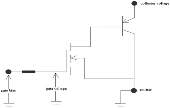
Figure 1.
The equivalent circuit for the IGBT modules.
The failure of the IGBT modules threatens the power grid reliability. Electric breakdown and thermal runaway are two main reasons for the IGBT failure [2,3]. The electric breakdown is caused by the surge of the collector voltage or the gate voltage. The thermal runaway is mainly due to the latch-up failure. In Figure 2, the outcome of the IGBT failures is illustrated [4]. Residual useful life (RUL) prediction can instruct the preventive replacement of the faulty IGBT modules, which prevents such a tragedy from happening [5].

Figure 2.
(left): IGBT module before failure; (right): IGBT module after failure.
The major control method for the IGBT modules is pulse-width modulation (PWM), which means the gate bias is a square wave [6]. When the gate bias is on the peak, the operation mode can switch between the active mode and the saturation mode. The IGBT module is operating on the forward locking mode if the control signal is on the trough. The output characteristics for the IGBT module are plotted in Figure 3. The threshold gate bias is the minimum gate bias to activate the IGBT module. The multi-modal characteristics complicate the IGBT degradation under PWM control. Therefore, RUL prediction for the PWM-controlled IGBT modules remains a promising but difficult task for the new energy power grid.
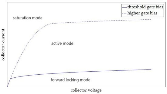
Figure 3.
Output characteristics of the IGBT modules.
1.2. Literature Review for Previous RUL Prediction Models of the IGBT Modules
The adaptability and accuracy of the model-based RUL prediction model is not satisfactory. The alternative methods are data-driven models, which utilize machine learning or the stochastic process to extract the degradation information.
Recently, several data-driven RUL prediction models have been proposed for the IGBT modules. An auxiliary particle filter (APF) is proposed to reduce the variance of the RUL prediction results [7]. In [8], a self-attention-based neural network (SA-NN) is used to automatically extract the features of IGBT degradation. The RUL prediction model based on machine learning requires a large quantity of training data, which may be difficult to acquire. In the optimal-scale Gaussian process model (OSGP), the parameters are optimized by the ant lion algorithm [9]. In [10], the Poisson process is used to establish a computationally efficient RUL prediction model (PCE). The Gaussian process and Poisson process are not suitable to describe the IGBT degradation data with non-Gaussian and non-Markovian characteristics.
1.3. Research Highlights
The degradation mechanism is different among different operation modes and, thus, the shifting of modes should be stressed in the RUL prediction models [11,12]. Considering both the modes of capacity decay and recovery, a nonlinear RUL prediction algorithm is proposed for the lithium battery in ref [13]. Ref. [14] proposes a RUL prediction algorithm based on fractional Lévy stable motion, in which three different modes of the steel furnace are considered. Multi-modal characteristics have been proven in the IGBT modules [15]. However, no previous RUL prediction models have stressed this phenomenon. In this paper, we use the Markovian mode transition process to characterize the multi-modal characteristics of the PWM-controlled IGBT modules, considering the memoryless effect of the grid operation.
Transfer learning is proposed for the estimation of the Markovian mode transition probabilities. The data from similar devices may have different data distributions due to the different health state and operation procedure. However, the connection between different data values is similar, which is transferrable among different data domains [16]. The only difference between the IGBT modules in the same batch of the experiment is the control signal, which satisfies the requirement of transfer learning. By transferring knowledge from similar equipment, the RUL prediction can achieve good results with little training data [17]. In [18], deep learning with an attention mechanism is combined with transfer learning for the RUL prediction of rocket engines. A long short-term memory neural network based on transfer learning has been used for long-term prediction of the lithium-ion battery capacity degradation [19].
To describe the non-Gaussian characteristics of the IGBT degradation, i.e., the skewness and heavy tail, fractional Weibull motion (fWm) is proposed. The non-Markovian property of the fWm, i.e., long-range dependence, is also analyzed. Long-range dependence indicates a strong temporal dependency for the time series [20]. The Hurst exponent of the long-range-dependent time series is within the interval of (0.5, 1). Degradation data from different modes are utilized to train the fWm of different modes. With the Markovian mode transition stochastic process, the fWm of multiple modes can be derived for the stochasticity modeling of the PWM-controlled IGBT modules.
As the environmental noise changes, the degrading rate of the IGBT modules varies. This phenomenon is not considered in the previous RUL prediction models. Ref. [21] proposes an adaptive RUL prediction model, in which the drift coefficient is updated with the random walk. An adaptive geometric fractional Lévy stable motion model is proposed based on the performance evaluation in [22]. In these models, the diffusion coefficient is presumed to be constant, which is a major drawback [23]. The PWM control signal can impact the variational speed of the IGBT degradation, which means the diffusion coefficient also needs to be updated. Considering the varying degradation pattern, both the drift and diffusion coefficients are adaptively updated in the current work.
A complex health indicator (CHI) is normally the weighed sum of different sensor data [24]. In [25], the CHI for the IGBT module is constructed by fusing the temperature and the collector voltage. The possible electric breakdown between the gate and the emitter is neglected. To construct a more comprehensive and informative CHI, a multi-sensor fusion algorithm is proposed in this work, combining the temperature, collector voltage and gate voltage.
1.4. Contributions of the Paper
Switching among multiple modes in the PWM-controlled IGBT module is modeled as the Markovian stochastic process. Transfer learning is employed for the estimation of the Markovian transition probabilities.
The fWm of multiple modes is proposed as the temporal variability in the multi-modal IGBT degradation. The drift and diffusion coefficients are adaptively updated in the RUL prediction model for the PWM-controlled IGBT module. A multi-sensor fusion algorithm is proposed to construct the CHI for the model training.
1.5. Structure of the Paper
The remainder of this paper is arranged as follows. In Section 2, transfer learning is introduced for the estimation of the Markovian transition probabilities. In Section 3, the fWm of multiple modes is utilized to model the stochasticity of the IGBT degradation with PWM control. The adaptive RUL prediction model is proposed in Section 4. In the case study, the multi-sensor fusion algorithm is employed to construct the CHI used in the model training. The main findings of this work are summarized in the Section 6.
2. Markovian Mode Transition Stochastic Process for the PWM-Controlled IGBT Module
2.1. Occurrence Probabilities Estimation for the PWM-Controlled IGBT Module
When the gate bias is direct voltage, the IGBT module is continuously switching between the active mode and the saturation mode. The collector voltage of an IGBT module with direct-voltage bias is depicted in Figure 4. As we can see from Figure 4, the difference between the active mode and the saturation mode is distinct. The collector voltage is higher on the active mode and lower on the saturation mode. In such a case, these two modes can be clearly identified and separated. Thus, we can estimate the occurrence probabilities of the active and saturation modes on the condition of direct-voltage bias as the occurrence frequencies.
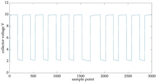
Figure 4.
Collector voltage of the IGBT module on the direct-voltage gate bias.
The PWM control signal for the IGBT module is a square wave, which is depicted in Figure 5. With the real PWM control signal, we can estimate the ratio of the peak and trough. For the PWM-controlled IGBT module, not all modes can be identified and separated. When the gate bias is on the peak, we can not determine whether the operation mode is the active mode or saturation mode. However, if the gate bias is on the trough, the current operation mode must be the forward locking mode. Therefore, we can identify and separate the forward locking mode from the whole signal, when the gate bias is on the trough.
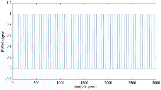
Figure 5.
The PWM control signal for the IGBT module.
The occurrence probabilities for the different modes in the PWM-controlled IGBT modules are
where mode 1 is the active mode, mode 2 is the saturation mode and mode 3 is the forward locking mode. and are the conditional probabilities for the active mode and the saturation mode. and are the ratio for the peak and the trough in the square wave, respectively.
2.2. Transfer Learning for the Construction of Markovian Mode Transition Stochastic Process
The mode shifting of the IGBT module is memoryless. Therefore, we consider the mode transition process as the Markovian stochastic process, which is described with the Markovian mode transition matrix.
The Markovian mode transition matrix is defined as the right stochastic matrix with non-negative probability values. The values in the row give the transition probabilities under the condition of a certain mode, with their summation to be one. The values in the column are the probabilities for the different modes to enter a certain mode.
The mode transition matrix for the IGBT module with direct-voltage gate bias is
where mode 1 is the active mode and mode 2 is the saturation mode.
The active mode and saturation mode can be clearly identified for the IGBT module with direct-voltage gate bias. Therefore, the mode transition probability can be estimated as the transition frequencies.
The mode transition matrix for the IGBT module with square-wave gate bias is defined as
where mode 1 is the active mode, mode 2 is the saturation mode and mode 3 is the forward locking mode.
The mode transition probabilities for the PWM-controlled IGBT module are difficult to estimate because not all the modes can be identified. Transfer learning is proposed to solve this problem. In the same batch of experiments, the IGBT modules are manufactured with a similar quality and procedure. The only difference is the control signal. Therefore, the transfer learning is applicable.
Prior transition probabilities among multiple modes can be calculated as the multiplication of the mode occurrence probabilities. The posterior transition probabilities related to the saturation and active modes are
where is the summation of the prior transition probabilities related to the saturation and active modes.
The Bayesian total probability formula and the properties of the Markovian transition matrix are utilized for the calculation of the other posterior probabilities.
3. Stochasticity Modeling of the Multi-Modal IGBT Degradation with the fWm
3.1. Statistical Properties of the fWm
The fWm is defined with the Riemann–Liouville integral and can be further expressed with convolution calculation:
where is the Hurst exponent, is white Weibull noise and is the convolution operator. A simulated path of the fWm is depicted in Figure 6.
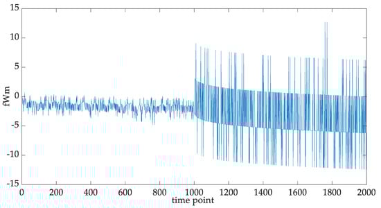
Figure 6.
Time series of the fWm.
The actual degradation data often present non-Gaussian characteristics, i.e., skewness and heavy tail. The fWm follows a Weibull assumption; therefore, it is more suitable to fit such kinds of degradation data.
Long-range dependence is beneficial to the stochasticity modeling of the degradation time series [26]. In light of the fractional Brownian motion [27], we give the long-range dependence criterion for the fWm here. If the Hurst exponent is 0.5, then the fWm time series is temporally independent. When the Hurst exponent is in the interval of (0.5, 1), the increments are positively correlated and, thus, the fWm time series is long-range-dependent. In such a case, positive (negative) increments are likely to be followed by the positive (negative) increments. The increments are negatively correlated if .
3.2. Stochaticity Modeling for the PWM-Controlled IGBT Modules with Multi-Modal fWm
Considering the multi-modal characteristics of the IGBT degradation, the fWm of multiple modes or multi-modal fWm is proposed for the stochasticity modeling of the degradation model, which is prepared in the following steps:
①: Separate the IGBT degradation data of different modes from the meta data.
②: Construct the CHI of different modes with a multi-sensor fusion algorithm. The CHI contains the information from multiple failure precursors, which makes it more comprehensive and informative.
③: Train the fWm of different modes with the CHI of different modes.
④: With the continuous mode switching, the fWm of multiple modes can be established. For each data point, its operation mode is determined with the Markovian mode transition stochastic process and its value is sampled from the fWm of the corresponding mode sequentially.
In Figure 7, the fWm of different modes is plotted. The fWm of multiple modes is depicted in Figure 8 and the mode dispersion plot is provided in Figure 9.
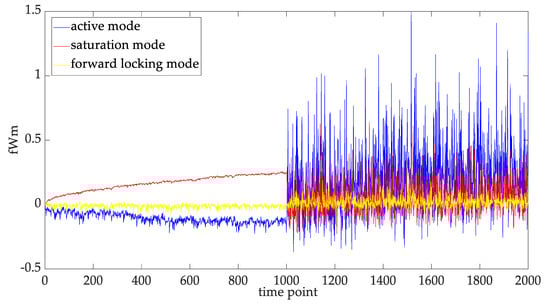
Figure 7.
The fWm of different operation modes.
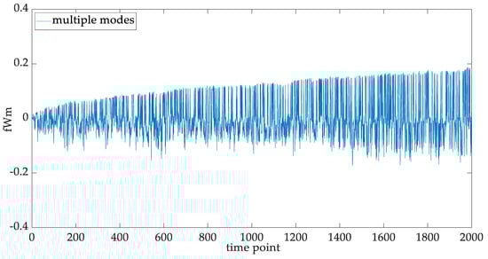
Figure 8.
The fWm of multiple modes.
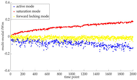
Figure 9.
Mode dispersion plot for the multi-modal fWm.
4. Adaptive RUL Prediction Model for the IGBT Module with PWM Control
4.1. Adaptive Degradation Model with Multiple Modes
We denote the degradation path with multiple modes as :
where is the drift coefficient, is the drift function, is the diffusion coefficient and is the fWm of multiple modes. The initial state is commonly zero.
The degradation speed of the IGBT module varies significantly in the different modes. Therefore, the switching of modes must be considered in the drift function, and this is conducted with the mode transition matrix. Under a certain degradation mode, the degradation rate is normally distributed, and the distribution parameters are estimated from the increments of the CHI values in the different modes. Then, the white Gaussian noise is used to construct the drift function:
During the mode shifting of the degradation process, various factors deviate the degradation pattern, e.g., changes in circuit topology and electric load. Therefore, the drift and diffusion coefficients must be adaptively updated.
The means of the drift and diffusion coefficients equal to one, representing the historical information. The variance of the drift coefficient is estimated from the CHI values in the different modes. The variance of the diffusion coefficient is estimated from the increments of the CHI values in the different modes.
Therefore, the multi-modal degradation path considering an adaptive mechanism is
The increments between two adjacent time points can be calculated as
where . The simulated path for the is provided in Figure 10.
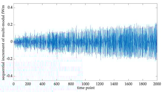
Figure 10.
The sequential increments of the multi-modal fWm.
Thus, the iterative representation of the degradation process with multiple modes is
In Figure 11, the multi-modal IGBT degradation path is plotted, which illustrates the degradation of the IGBT module with PWM control. The corresponding mode dispersion plot is provided in Figure 12.
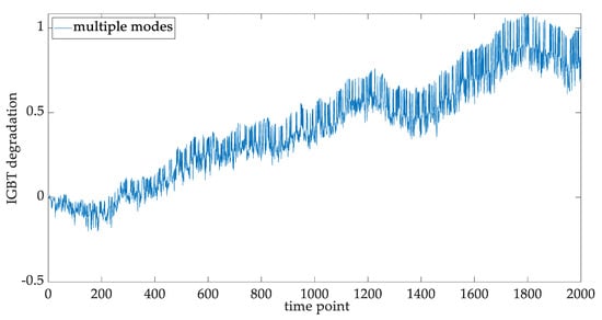
Figure 11.
IGBT degradation of multiple modes.
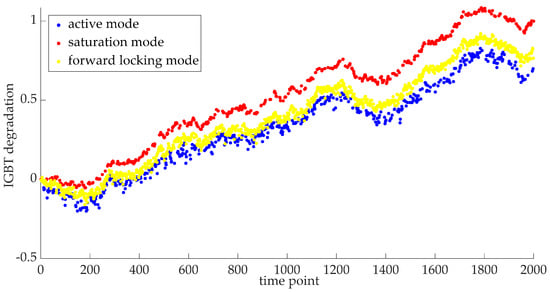
Figure 12.
Mode dispersion plot in the multi-modal IGBT degradation.
4.2. Adaptive RUL Prediction Model for the PWM-Controlled IGBT Module
The failure mechanism of different modes is different, which means the failure threshold (FT) should be different. The end of life (EOL) of a single mode is defined as the first passage of time for the degradation path to exceed the corresponding FT:
where is the EOL of a certain mode and is the FT of a certain mode.
For the IGBT module with PWM control, exceeding the FT in one or two modes is not sufficient for the failure. Only when all three modes of the IGBT degradation exceed their exclusive FT can we determine the EOL for the multi-modal IGBT degradation. Thus, the multi-modal EOL is
A flow chart of the proposed RUL prediction model is plotted in Figure 13. The multiple modes are separated from the meta data and the CHI is, then, constructed through the multi-sensor fusion. If the Hurst exponents of different modes are larger than 0.5, then the long-range dependence criterion for the RUL prediction model is satisfied.
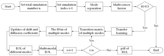
Figure 13.
Flowchart of the adaptive RUL prediction model.
Transfer learning is employed to estimate the transition matrix of multiple modes.
The fWm of multiple modes introduces the temporal variability to the degradation model. The drift and diffusion coefficients are adaptively updated with the evolution of the random walk. The EOL values of different modes are calculated separately, and the maximum is the EOL of multiple modes. Due to the stochasticity of the degradation process, the RUL prediction outcome is in terms of a probability density function (pdf) based on a Monte Carlo simulation. The mean value of the pdf can be considered as the point prediction.
5. Case Study
5.1. The Thermal-Accelerated IGBT Aging Data
The thermal-accelerated IGBT aging dataset is provided by NASA [28]. The cause of IGBT failure in the experiment is the latch-up failure and the following thermal runaway. Two sets of IGBT degradation data are utilized in this work. The first set is the aging data collected from an IGBT module with direct-voltage gate bias, which is the source domain for the knowledge extraction. The second set is the aging data acquired from an IGBT module with PWM control, which is the target domain for the transfer learning. The collector voltage, gate voltage and temperature of both datasets are depicted in Figure 14 and Figure 15, made with matlab software 2022b.
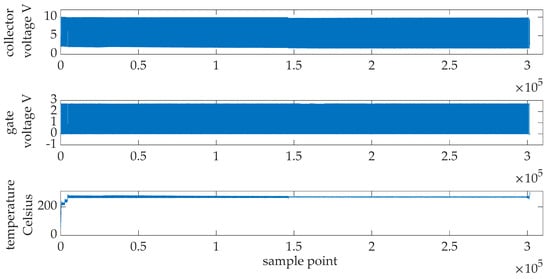
Figure 14.
Degradation data from the IGBT module with direct-voltage gate bias.
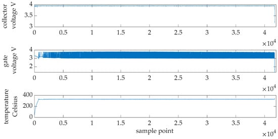
Figure 15.
Degradation data from the PWM-controlled IGBT module.
5.2. Mode Separation for the IGBT Degradation Data
For the construction of the CHI, different degradation modes should be separated. The degradation data of the active mode and saturation mode are separated from the IGBT module with direct-voltage gate bias (see Figure 16). The degradation data of the forward locking mode is separated from the PWM-controlled IGBT module and depicted in Figure 17.
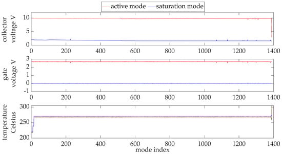
Figure 16.
IGBT degradation data of active and saturation modes.
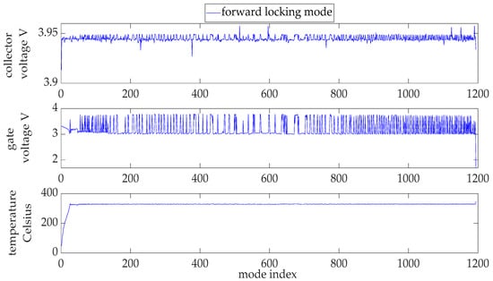
Figure 17.
IGBT degradation data of forward locking mode.
5.3. Multi-Sensor Fusion for the CHI Construction
The formulation of the CHI on a certain mode is
where is the weight of the collector voltage , is the weight of the gate voltage and is the weight of the temperature .
The weight calculation formulas are
where expresses the quantitative relationship between the voltages in the IGBT module due to Kirchhoff’s laws. Both the collector and gate voltages contribute to the temperature rising.
The CHI of different modes is normalized and then plotted in Figure 18, Figure 19 and Figure 20, in which we can visualize the degradation trend. The failure points of different modes are also pointed out and the corresponding data values are the FT of different modes.
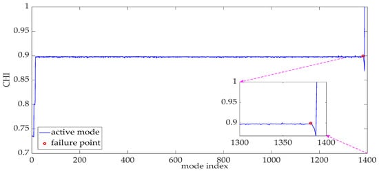
Figure 18.
CHI of the active mode.
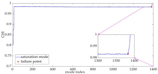
Figure 19.
CHI of the saturation mode.
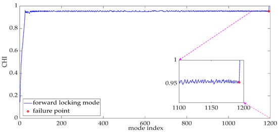
Figure 20.
CHI of the forward locking mode.
5.4. Statistical Fitting of the Multi-Modal IGBT Degradation
Weibull distribution, exponential distribution, Gaussian distribution and lognormal distribution are utilized in the fitting experiment of the IGBT degradation data [29]. The root mean-squared error (RMSE) and the determination coefficient are chosen as the evaluation metrics. Smaller values of the RMSE and higher values of the imply better fitting results. The fitting results are compiled in Table 1, Table 2 and Table 3. Because the best fitting distribution is the Weibull distribution, it is appropriate to use the fWm to model the stochasticity of the IGBT degradation.

Table 1.
Statistical fitting results for the degradation data in the active mode.
Table 2.
Statistical fitting results for the degradation data in the saturation mode.
Table 3.
Statistical fitting results for the degradation data in the forward locking mode.
5.5. Statistical Properties of the Multi-Modal IGBT Degradation
The augmented Dickey–Fuller test is conducted, which shows that the degradation data are nonstationary [30]. Thus, the wavelet variance algorithm is utilized for the calculation of Hurst exponents (see Figure 21) [31]. The skewness and kurtosis values are also calculated for the different modes. The Hurst exponents, skewness values and kurtosis values are summarized in Table 4.
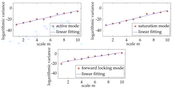
Figure 21.
Logarithmic linear regressions for the estimation of Hurst exponents.
Table 4.
Statistical metrics of the degradation data in different modes.
5.6. Performance Evaluation of the Proposed RUL Prediction Model
The RUL prediction results based on the multi-modal fWm are plotted in Figure 22. The APF model, SA-NN model, OSGP model and PCE model are used for the model comparison (see Figure 23). The point predictions are illustrated in Figure 24.
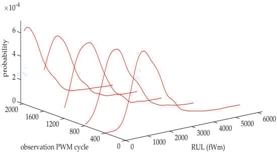
Figure 22.
RUL prediction based on fWm of multiple modes.
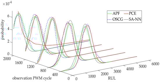
Figure 23.
RUL predictions for comparison.
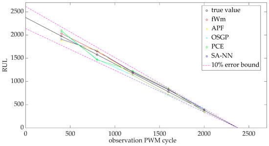
Figure 24.
Point RUL predictions.
The boxplot of the relative prediction error is depicted in Figure 25. In Table 5, the maximum relative prediction error, mean relative prediction error, standard deviation (std), mean absolute error (MAE) and RMSE are compiled.
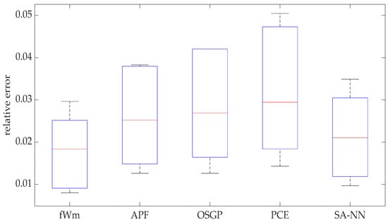
Figure 25.
Boxplot of the relative prediction error.
Table 5.
Statistical metrics of the predictive error.
6. Conclusions
In this work, an adaptive RUL prediction model is proposed for the IGBT module with PWM control. The model training is conducted with the output of the multi-sensor fusion algorithm.
The IGBT operation under PWM control features multi-modal characteristics, which can be modeled with the Markovian mode transition stochastic process. Transfer learning is employed to estimate the Markovian transition probabilities. The fWm of multiple modes is utilized to model the stochasticity of the multi-modal IGBT degradation. The drift and diffusion coefficients in the degradation model are adaptively updated with the evolution of the random walk.
In the future, we are determined to extend the proposed model to the RUL prediction of other electric components, e.g., lithium batteries and supercapacitor and light-emitting diodes, in which the multi-modal characteristics can also be found [32,33,34].
Supplementary Materials
The following supporting information can be downloaded at: https://www.mdpi.com/article/10.3390/fractalfract7080614/s1. The research data in the Supplementary Materials are public data provided by the research institute of NASA.
Author Contributions
Conceptualization, Y.G.; methodology, W.D. and Y.G.; software, W.D.; validation, E.Z. and A.K.; formal analysis, Y.G.; investigation, W.S.; resources, W.S.; data curation, E.Z., G.L. and A.K.; writing—original draft preparation, W.D.; writing—review and editing, E.Z.; visualization, W.D.; supervision, G.L. and J.L.; project administration, W.S., G.L. and J.L.; funding acquisition, J.L. and A.K. All authors have read and agreed to the published version of the manuscript.
Funding
This research received no external funding.
Data Availability Statement
The research data can be found in the Supplementary Materials.
Acknowledgments
We thank the experimental assistance from the Shanghai University of Engineering Science.
Conflicts of Interest
The authors declare no conflict of interest.
Abbreviations
| IGBT | insulated-gate bipolar transistor |
| PWM | pulse-width modulation |
| RUL | residual useful life |
| APF | auxiliary particle filter |
| SA-NN | self-attention-based neural network |
| OSGP | optimal scale Gaussian process model |
| PCE | Poisson computationally efficient model |
| fWm | fractional Weibull motion |
| CHI | complex health indicator |
| FT | failure threshold |
| EOL | end of life |
| probability density function | |
| RMSE | root mean-squared error |
| MAE | mean absolute error |
| std | standard deviation |
References
- Han, L.B.; Liang, L.; Kang, Y.; Qiu, Y.F. A Review of SiC IGBT: Models, Fabrications, Characteristics, and Applications. IEEE Trans. Power Electron. 2020, 36, 2080–2093. [Google Scholar] [CrossRef]
- Oh, H.; Han, B.; McCluskey, P.; Han, C.; Youn, B.D. Physics-of Failure, Condition Monitoring and Prognostics of Insulated Gate Bipolar Transistor Modules: A Review. IEEE Trans. Power Electron. 2014, 30, 2413–2426. [Google Scholar] [CrossRef]
- Mauro, C. Selected failure mechanisms of modern power modules. Microelectron. Reliab. 2002, 42, 653–667. [Google Scholar] [CrossRef]
- Fischer, K.; Pelka, K.; Puls, S.; Poech, M.H.; Mertens, A.; Bartschat, A.; Tegtmeier, B.; Broer, C.; Wenske, J. Exploring the Causes of Power-Converter Failure in Wind Turbines based on Comprehensive Field-Data and Damage Analysis. Energies 2019, 12, 593. [Google Scholar] [CrossRef]
- Lei, Y.G.; Li, N.P.; Guo, L.; Li, N.B.; Yan, T.; Lin, J. Machinery health prognostics: A systematic review from data acquisition to RUL prediction. Mech. Syst. Signal Process. 2018, 104, 799–834. [Google Scholar] [CrossRef]
- Wu, M.Z.; Li, Y.W.; Konstantinou, G. A Comprehensive Review of Capacitor Voltage Balancing Strategies for Multilevel Converters Under Selective Harmonic Elimination PWM. IEEE Trans. Power Electron. 2020, 36, 2748–2767. [Google Scholar] [CrossRef]
- Moinul, S.H.; Seungdeng, C.; Jeihoon, B. Auxiliary Particle Filtering-Based Estimation of Remaining Useful Life of IGBT. IEEE Trans. Power Electron. 2018, 65, 2693–2703. [Google Scholar] [CrossRef]
- Xiao, D.Y.; Qin, C.J.; Ge, J.W.; Xie, P.C.; Huang, Y.X.; Liu, C.L. Self-attention-based adaptive remaining useful life prediction for IGBT with Monte Carlo drop-out. Knowl.-Based Syst. 2022, 239, 107902. [Google Scholar] [CrossRef]
- Li, L.L.; Zhang, X.B.; Tseng, M.L.; Zhou, Y.T. Optimal scale Gaussian process regression model in Insulated Gate Bipolar Transistor remaining life prediction. Appl. Soft Comput. 2019, 78, 261–273. [Google Scholar] [CrossRef]
- Alghassi, A.; Perinpanayagam, S.; Samie, M.; Screenuch, T. Computationally Efficient, Real-Time, and Embeddable Prognostic Techniques for Power Electronics. IEEE Trans. Power Electron. 2015, 30, 2623–2634. [Google Scholar] [CrossRef]
- Xi, X.; Zhou, D.; Chen, M.; Balakrishnan, N. Remaining useful life prediction for fractional degradation processes under varying modes. Can. J. Chem. Eng. 2020, 98, 1351–1364. [Google Scholar] [CrossRef]
- Zhang, H.W.; Zhou, D.H.; Chen, M.Y.; Shang, J. FBM-Based Remaining Useful Life Prediction for Degradation Processes With Long-Range Dependence and Multiple Modes. IEEE Trans. Reliab. 2018, 68, 1021–1033. [Google Scholar] [CrossRef]
- Zhang, Z.Y.; Peng, Z.; Guan, Y.; Wu, L.F. A Nonlinear Prediction Method of Lithium-ion Battery Remaining Useful Life Considering Recovery Phenomenon. Int. J. Electrochem. Sci. 2020, 15, 8674–8693. [Google Scholar] [CrossRef]
- Duan, S.W.; Song, W.Q.; Zio, E.; Cattani, C.; Li, M. Product technical life prediction based on multi-modes and fractional Levy stable Motion. Mech. Syst. Signal Process. 2021, 161, 107974. [Google Scholar] [CrossRef]
- Rahimo, M.T.; Shammas, N.Y.A. Freewheeling diode reverse-recovery failure modes in IGBT applications. IEEE Trans. Ind. Appl. 2021, 37, 661–670. [Google Scholar] [CrossRef]
- Hao, J.; Rongshun, J.; Randy, G.; Keisuke, N.; Guangliang, L. Transferring policy of deep reinforcement learning from simulation to reality for robotics. Nat. Mach. Intell. 2022, 4, 1077–1087. [Google Scholar] [CrossRef]
- Ding, Y.F.; Jia, M.P.; Miao, Q.H.; Huang, P. Remaining useful life estimation using deep metric transfer learning for kernel regression. Reliab. Eng. Syst. Saf. 2021, 212, 107583. [Google Scholar] [CrossRef]
- Pan, T.Y.; Chen, J.L.; Ye, Z.S.; Li, A.M. A multi-head attention network with adaptive meta-transfer learning for RUL prediction of rocket engines. Reliab. Eng. Syst. Saf. 2022, 225, 108610. [Google Scholar] [CrossRef]
- Pan, D.W.; Li, H.F.; Wang, S.J. Transfer Learning-Based Hybrid Remaining Useful Life Prediction for Lithium-Ion Batteries Under Different Stresses. IEEE Trans. Instrum. Meas. 2022, 71, 3501810. [Google Scholar] [CrossRef]
- Makogin, V.; Oesting, M.; Rapp, A.; Spodarev, E. Long range dependence for stable random processes. J. Time Ser. Anal. 2020, 42, 161–185. [Google Scholar] [CrossRef]
- Wang, W.B.; Carr, M.; Xu, W.J.; Kobbacy, K. A model for residual life prediction based on Brownian motion with an adaptive drift. Microelectron. Reliab. 2011, 51, 285–293. [Google Scholar] [CrossRef]
- Li, Q.; Ma, Z.H.; Li, H.K.; Liu, X.J.; Guan, X.C.; Tian, P.H. Remaining useful life prediction of mechanical system based on performance evaluation and geometric fractional Lévy stable motion with adaptive nonlinear drift. Mech. Syst. Signal Process. 2023, 184, 109679. [Google Scholar] [CrossRef]
- Wang, H.; Ma, X.B.; Zhao, Y. An improved Wiener process model with adaptive drift and diffusion for online remaining useful life prediction. Mech. Syst. Signal Process. 2019, 127, 370–387. [Google Scholar] [CrossRef]
- Li, T.M.; Si, X.S.; Pei, H.; Sun, L. Data-model interactive prognosis for multi-sensor monitored stochastic degrading devices. Mech. Syst. Signal Process. 2022, 167, 108526. [Google Scholar] [CrossRef]
- Rao, Z.; Huang, M.; Zha, X.M. IGBT Remaining Useful Life Prediction Based on Particle Filter With Fusing Precursor. IEEE Access 2020, 8, 154281–154289. [Google Scholar] [CrossRef]
- Bayraktav, E.; Poor, V.H.; Rao, R. Prediction and tracking of long-range dependent sequences. Syst. Control Lett. 2005, 54, 1083–1090. [Google Scholar] [CrossRef]
- Li, K.X. Stochastic delay fractional evolution equations driven by fractional Brownian motion. Math. Methods Appl. Sci. 2015, 38, 158291. [Google Scholar] [CrossRef]
- Sonnenfeld, G.; Goebel, K.; Celaya, J. An Agile Accelerated Aging, Characterization and Scenario Simulation System for Gate Controlled Power Transistors. In Proceedings of the 43rd Annual IEEE AUTOTESTCON Conference, Salt Lake City, UT, USA, 31 October 2008. [Google Scholar] [CrossRef]
- Chen, Z.H.; Zheng, S.R. Lifetime Distribution Based Degradation Analysis. IEEE Trans. Reliab. 2005, 54, 3–10. [Google Scholar] [CrossRef]
- Paparoditis, E.; Politis, D.N. The asymptotic size and power of the augmented Dickey-Fuller test for a unit root. Econom. Rev. 2018, 37, 955–973. [Google Scholar] [CrossRef]
- Serroukh, A.; Walden, A.T.; Percival, D.B. Statistical Properties and Uses of the Wavelet Variance Estimator for the Scale Analysis of Time Series. J. Am. Stat. Assoc. 2000, 95, 184–196. [Google Scholar] [CrossRef]
- Chaari, R.; Briat, O.; Vinassa, J.M. Capacitance recovery analysis and modelling of supercapacitors during cycling ageing tests. Energy Convers. Manag. 2014, 82, 37–45. [Google Scholar] [CrossRef]
- Rao, K.S.; Mohapatra, Y.N. Disentangling degradation and auto-recovery of luminescence in Alq(3) based organic light emitting diodes. J. Lumin. 2014, 145, 793–796. [Google Scholar] [CrossRef]
- Kleeberger, V.B.; Barke, M.; Werner, C.; Schmitt, L.D.; Schlichtmann, U. A compact model for NBTI degradation and recovery under use profile variations and its application to aging analysis of digital integrated circuits. Microelectron. Reliab. 2014, 54, 1083–1089. [Google Scholar] [CrossRef]


Disclaimer/Publisher’s Note: The statements, opinions and data contained in all publications are solely those of the individual author(s) and contributor(s) and not of MDPI and/or the editor(s). MDPI and/or the editor(s) disclaim responsibility for any injury to people or property resulting from any ideas, methods, instructions or products referred to in the content. |
© 2023 by the authors. Licensee MDPI, Basel, Switzerland. This article is an open access article distributed under the terms and conditions of the Creative Commons Attribution (CC BY) license (https://creativecommons.org/licenses/by/4.0/).