Abstract
In this paper, we solve the space fractional nonlinear Schrödinger equation (SFNSE) by developing an explicit–implicit spectral element scheme, which is formulated based on the Legendre spectral element approximation in space and the Crank–Nicolson leap frog (CNLF) difference discretization in time. Both mass and energy conservative properties are discussed for the spectral element scheme. Numerical stability and convergence of the scheme are proved. Numerical experiments are performed to confirm the high accuracy and efficiency of the proposed numerical scheme.
Keywords:
space fractional Schrödinger equation; spectral element method; mass and energy conservation; stability and convergence MSC:
26A33; 65M70; 65M12
1. Introduction
Fractional differential equations (FDEs) have played a very important role in the simulation of practical problems in science and engineering. Because of the existing fractional derivatives, it is difficult to solve most FDEs by making use of analytical methods for researchers. So, more and more scholars have begun to pay attention to numerical methods for solving different FDEs, such as (discontinuous) Galerkin finite element methods [1,2,3,4,5], finite difference methods [6,7], meshless methods [8], finite volume methods [9,10] and spectral methods [11,12,13,14]. Based on the literature, scholars can see that the studies of different numerical methods of fractional equations have been much concerned.
The fractional Schrödinger equation is yielded by the classical Schrödinger equation, which plays an important role in quantum mechanics and has many applications in the field, such as in nonlinear optics, plasma physics and fluid dynamics [15,16,17,18,19,20]. Naber [21] first deduced the time fractional Schrödinger equation [22,23], where the first-order time derivative was substituted by the Caputo fractional derivative. Laskin created the spatial fractional Schrödinger equation, an extension of the traditional Schrödinger equation. This is achieved by replacing the second-order spatial derivative with a Riesz fractional derivative [24,25]. Guo [26] proved the existence of a global smooth solution of the fractional nonlinear Schrödinger equation with periodic boundary conditions.
In this paper, we consider the following SFNSE:
with the initial and Dirichlet boundary conditions given by
where , and is a real constant. Suppose that the solution of the system (1)–(3) is small outside of the interval , which can be neglected, i.e.,
The Riesz space fractional derivative is defined as [27]
where and are the left and right Riemann–Liouville fractional derivatives defined as follows:
Due to the existence of the nonlinear term, it is difficult to obtain the solution of the SFNSE exactly; thus, numerical methods for solving the SFNSE have been studied by many authors, such as finite difference method [6,28,29,30,31,32,33], finite element method [34,35,36,37], spectral method [22,38,39,40] and other methods [41]. Li and Wang [42] and Li et al. [43] utilized this method for solving the integer-order nonlinear Schrödinger equation. However, we have not seen any relevant reports on the spectral element method for solving SFNSE.
As is known to all, the spectral element method was yielded by the combination of the finite element method and the spectral method, which means that it incorporates the higher-order accuracy of the spectral method and the geometric flexibility of the finite element scheme. Recently, the spectral element method has been applied for solving FDEs such as the neutral time delay distributed-order fractional damped diffusion-wave equation [44] and the 2D multiterm time-fractional diffusion-wave equation [45]. In 2018, Mao and Shen developed the spectral element method for solving two-sided space FDEs in 1D [46] with geometric mesh.
According to the references above, one can see that the spectral element method is mainly solving integer DEs, time FDEs and 1D linear space FDEs. It is urgent to develop this method to nonlinear cases. To our knowledge, the spectral element method for solving the SFNSE is still blank. This is why we choose the spectral element method, as it is a starting point for solving the one-dimensional SFNSE, and we will extend this method to solve this type of equation on irregular domains in the future.
This study introduces a fresh numerical method for solving spatial fractional Schrödinger equations aimed at narrowing the gap in this area of research. We use Legendre spectral element approximation in space following the idea proposed by Mao and Shen [46], which considered the linear space FDEs in 1D, as well as CNLF difference discretization in time just like Refs. [33,47], as we know the CNLF scheme can reach the accuracy .
Our major contributions are highlighted as follows:
- We create a fully discrete explicit–implicit CNLF-type spectral element scheme for solving the SFNSE.
- The spectral element scheme satisfies both the mass conservation and energy conservation laws, which is compatible with the property of the SFNSE itself.
- Stability and convergence theorems of the spectral element scheme are rigorously proved; we obtain an optimal error estimation and present numerical experiments to confirm our theoretical result.
The outline is organized as follows. Some preliminaries and notations are shown in Section 2. In Section 3, we build a fully discrete spectral element scheme for the SFNSE, analyze the scheme that satisfies both the mass conservation and energy conservation, and also prove the stability and convergence of the fully discrete scheme. Numerical experiments evaluate the effectiveness and the efficiency of the CNLF-type spectral element scheme in Section 4. Finally, some conclusions are made in Section 5.
2. Preliminaries and Notations
Let be the inner product on the space with the norm —that is,
Let be a non-negative real number; we use and as the usual Sobolev spaces with the norm and the seminorm . c is consistently used to stand for a generic positive constant independent of N.
In the sequel, we list some fractional spaces and , which we will use hereafter (see [48,49] for more detail).
Definition 1.
Let ; we define the seminorm
and the norm
and denote as the closure of with respect to , where is the space of smooth functions with compact support in
Definition 2.
Let ; we define the seminorm
and the norm
and denote as the closure of with respect to .
Definition 3.
Let and ; we define the seminorm
and the norm
and denote as the closure of with respect to .
Definition 4.
For we define the seminorm
and the norm
where ξ and stand for the Fourier transform parameter and the Fourier transform of u, respectively. Denote as the closure of with respect to .
For the properties of the norms and seminorms defined in the above definitions, we have the following lemma (see [48,49] for more detail).
Lemma 1.
Suppose and ; then, , and are equal with equivalent norms and seminorms. and are equal with equivalent norms and seminorms.
The following Gronwall inequality will be used.
Lemma 2
(see [50]). Assume that , are non-negative sequences and satisfies
Then it follows that
3. The Fully Discrete Scheme
In this section, we mainly give the fully discrete scheme for (1)–(3) and discuss the conservation laws of the scheme. In order to obtain the variational formulation of (1)–(3), we first introduce the following lemma.
Lemma 3
(See [51]). For if and then
For convenience, we define the following seminorm and norm:
As is known, the standard spectral Galerkin method is not very suitable for fractional partial differential equations with singularities due to the high requirement of smoothness of the equation. However, the spectral element method is qualified to deal with singularities at endpoints effectively.
Divide the domain into non-overlapping uniform elements:
where h is the length of the element, N is a positive integer and stands for the space of all polynomials with a degree no greater than N. represents the approximation space, which can be expressed as
and
For the interior unknowns in each subdomain, we adopt the base functions , which are composed of Legendre polynomials , in space as follows:
where . For the unknowns at the nodes we define the function :
Then, we can write
Let represent the time step size and M be a positive integer with and for . Denote and
Now, we present the CNLF-type spectral method for (1)–(3).
where is an appropriate projection operator and its relevant properties are shown in Section 3.2.
3.1. Mass Conservation and Energy Conservation
The fully discrete scheme (10) satisfies both the mass conservation and energy conservation laws. Now, we consider these two conservation laws carefully.
Lemma 4.
For the discrete solution , , we have
Proof.
Taking the real part of the above inequality, we obtain the desired result. □
Theorem 1.
The fully discrete scheme (10) satisfies the following two conservation laws:
and
where
Proof.
Setting in (10), we obtain
Taking the imaginary part of Equation (12), we have
Thus, we obtain the mass conservation law. Now, we prove the energy conservation law. Letting , we have
Taking the real part of Equation (13), we obtain
Thus, we have
Finally, we obtain the desired result. □
Remark 1.
Theorem 1 indicates that the fully discrete spectral element scheme (10) is unconditionally stable in the sense.
3.2. Convergence
In this subsection, we prove the convergence for the spectral element scheme (10). Before we prove the convergence theorem, we first introduce the following orthogonal projection operator : , which is defined as
It is obvious that by taking and using the properties of B, we have
For the property of the projection , we have the following lemma.
Lemma 5
(see [52]). Let r be a real number satisfying ; if the following estimate holds:
where C is a positive constant that is independent of N.
For the orthogonal projection approximation result of the spectral method, we refer to [39].
Theorem 2.
Suppose that the exact solution u of the system (1)–(3) satisfies , and Then, we have
where C is independent of τ and N.
Proof.
Denote
Subtracting (10) from (6) and using the definition of , we obtain the error equation as follows:
Letting in (16), then taking the imaginary part, we infer that
Next, we estimate the right term of Equation (17) for the case . According to Hölder’s inequality, Young’s inequality, Lemma 5 and the following equalities estimated by Taylor expansion,
and
we deduce
and
Substituting the above three estimates into (17), noting that , and summing up k from 1 to , we infer that
For the estimate , by Taloy’s expansion , we obtain
With a sufficiently small , using Gronwall inequality, we infer that
Similar to the procedure above, we obtain the following conclusion when :
By the triangle inequality and Lemma 5, we finally obtain the theoretical result. □
4. Numerical Results
In this section, we carry out numerical experiments by using the spectral element scheme (10) and (11) to verify our theoretical results.
4.1. Numerical Implementation
From Equation (10), we have
Note that it is difficult to calculate the nonlinear terms in a straightforward manner. Thus, we use the Gauss integral formula to calculate the nonlinear terms. Substituting defined by Equation (9) into Equation (20) and letting run through all basis functions of , we obtain the following system:
where
M is the mass matrix and, by the definition of the basis functions, we obtain
where
By the definition of the basis functions, we have
According to the orthogonality of Legendre polynomials, we obtain
For , we calculate it by arguing as follows:
If ,
If ,
If ,
We can calculate the last integral by the Legendre–Gauss quadrature. By the definition of , we also find that . For the matrix , we obtain
and are the corresponding left and right fractional Riemann–Liouville stiff matrices, respectively. It is easy to check that
is a block matrix defined by
where
are corresponding modal–modal, nodal–nodal, modal–nodal and nodal–nodal block stiff matrices [46]. Comparing the trivial computation of mass matrix M and C, it is non-trivial to compute efficiently because of the non-local properties of the fractional derivative. Following the idea of [46], we can use uniform mesh instead of geometric mesh.
4.2. Numerical Results
In this subsection, to validate the effectiveness of the presented algorithm, we choose the following SFNSE (1):
First, we define the convergence rates in time and space in the -norm sense as the following:
Due to there being no exact solution to problem (22) for , we approximate the error as error () We take and ; then, the numerical solutions to problem (22) with different are depicted in Figure 1. We observe that the shape of the solution will be affected by the order . When becomes smaller, the shape of the solution will change more quickly; when tends to 2, the numerical solutions are convergent to the solutions of the usual classical integer one. This property of the fractional Schrödinger equation can be used in physics to modify the shape of the wave without changing the nonlinearity and dispersion effects, readers can refer to [29] for more detail.
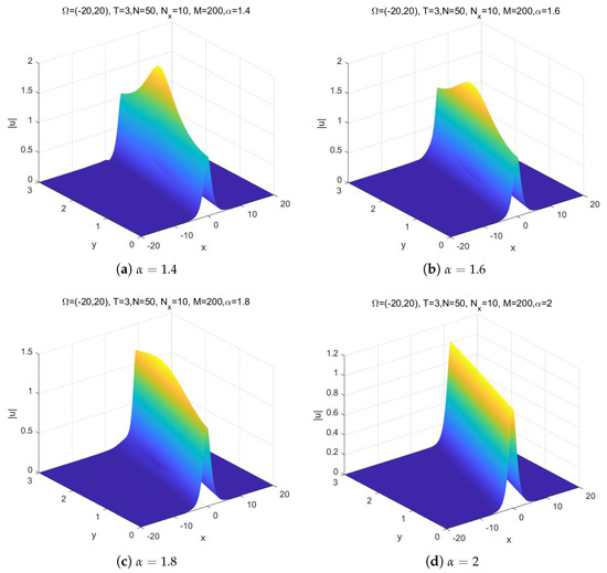
Figure 1.
Numerical solution of problem (22) with different .
We also test the time accuracy and space accuracy with the parameters , respectively. Table 1 shows that the errors and order versus of -norm with for , respectively. We obtain that the second-order accuracy in time is observed for -error.

Table 1.
The errors and order versus of -norm for different when .
In Figure 2, we plot the -errors versus N with for , respectively. The picture indicates an exponential convergence rate, which is the so-called spectral accuracy. It is obvious that our numerical results are in agreement with the theoretical analysis.
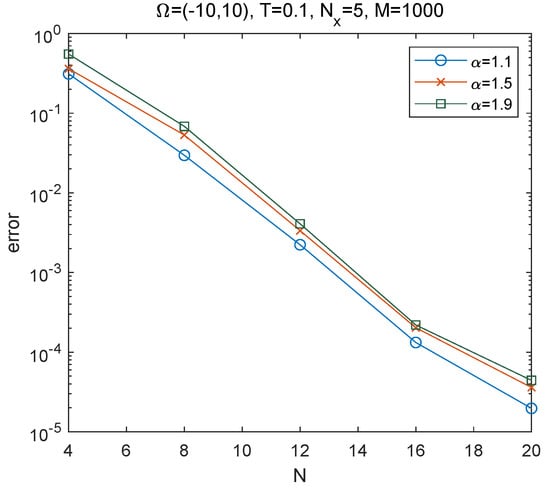
Figure 2.
-errors versus N with for different for problem (22).
We also test the mass conservation and energy conservation. Figure 3 shows the evolution of mass and energy. We can see that the three curves of the left picture in Figure 3 overlap with each other, which further illustrates that the mass only depends on the initial values and is unaffected by different ; thus, we deduce that the numerical experiments coincide with Theorem 1.
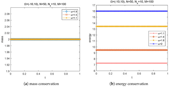
Figure 3.
Mass conservation and energy conservation.
All the numerical results are all consistent with our theoretical analysis.
5. Conclusions
In this paper, for solving the SFNSE, we establish an explicit–implicit discrete spectral element scheme formulated by combining the temporal CNLF scheme with the spectral element algorithm. From the numerical results, one can see that the scheme we consider in this paper satisfies both the mass conservation and energy conservation laws. Further, the stability and convergence are also analyzed. Numerical experiments are shown to illustrate the effectiveness of the considered numerical algorithm. In addition to the current study, in the future, this developed method will be applied to high-dimensional cases with irregular domains and coupled space fractional Schrödinger equations [28].
Author Contributions
Methodology, Z.L.; software, B.Y.; validation, Y.L.; formal analysis, Z.L. and Y.L.; data curation, B.Y. and Y.L.; writing—original draft, Z.L.; writing—review and editing, B.Y. and Y.L.; funding acquisition, Z.L. All authors have read and agreed to the published version of the manuscript.
Funding
This work was supported by the Fundamental Research Funds for the Central Universities (Nos. 2022YB007, 2020060).
Data Availability Statement
All the required data is included within the manuscript.
Acknowledgments
We would like to express our gratitude to the editors and four anonymous referees whose constructive comments were very helpful for improving the quality of our paper.
Conflicts of Interest
The authors declare that they have no conflict of interest.
References
- Liu, Y.; Fan, E.Y.; Yin, B.L.; Li, H.; Wang, J.F. TT-M finite element algorithm for a two-dimensional space fractional Gray-Scott model. Comput. Math. Appl. 2020, 80, 1793–1809. [Google Scholar] [CrossRef]
- Shi, D.; Yang, H. Superconvergence analysis of finite element method for time-fractional thermistor problem. Appl. Math. Comput. 2018, 323, 31–42. [Google Scholar] [CrossRef]
- Li, C.P.; Wang, Z. The discontinuous Galerkin finite element method for Caputo-type nonlinear conservation law. Math. Comput. Simul. 2020, 169, 51–73. [Google Scholar] [CrossRef]
- Feng, L.; Liu, F.; Turner, I.; Yang, Q.; Zhuang, P. Unstructured mesh finite difference/finite element method for the 2D time-space Riesz fractional diffusion equation on irregular convex domains. Appl. Math. Model. 2018, 59, 441–463. [Google Scholar] [CrossRef]
- Bu, W.P.; Tang, Y.F.; Yang, J.Y. Galerkin finite element method for two-dimensional Riesz space fractional diffusion equations. J. Comput. Phys. 2014, 276, 26–38. [Google Scholar] [CrossRef]
- Yin, B.L.; Wang, J.F.; Liu, Y.; Li, H. A structure preserving difference scheme with fast algorithms for high dimensional nonlinear space-fractional Schrödinger equations. J. Comput. Phys. 2021, 425, 109869. [Google Scholar] [CrossRef]
- Ding, H.; Li, C. Fractional-compact numerical algorithms for Riesz spatial fractional reaction-dispersion equations. Fract. Calc. Appl. Anal. 2017, 20, 722–764. [Google Scholar] [CrossRef][Green Version]
- Abbaszadeh, M.; Dehghan, M. Meshless upwind local radial basis function-finite difference technique to simulate the time-fractional distributed-order advection-diffusion equation. Eng. Comput. 2021, 37, 873–889. [Google Scholar] [CrossRef]
- Liu, F.; Turner, I.; Anh, V.; Su, N. A two-dimensional finite volume method for transient simulation of time-and scale-dependent transport in heterogeneous aquifer systems. J. Appl. Math. Comput. 2003, 11, 215–241. [Google Scholar] [CrossRef]
- Zheng, X.C.; Liu, H.; Wang, H.; Fu, H.F. An efficient finite volume method for nonlinear distributed-order space-fractional diffusion equations in three space dimensions. J. Sci. Comput. 2019, 80, 1395–1418. [Google Scholar] [CrossRef]
- Liu, Z.; Liu, F.; Zeng, F. An alternating direction implicit spectral method for solving two dimensional multi-term time fractional mixed diffusion and diffusion-wave equations. Appl. Numer. Math. 2019, 136, 139–151. [Google Scholar] [CrossRef]
- Liu, Z.; Lü, S.; Liu, F. Fully discrete spectral methods for solving time fractional nonlinear Sine-Gordon equation with smooth and non-smooth solutions. Appl. Math. Comput. 2018, 333, 213–224. [Google Scholar] [CrossRef]
- Liu, Z.; Lü, S. Hermite Pseudospectral method for the time fractional diffusion equation with variable coefficients. Int. J. Nonlinear Sci. Numer. Simulat. 2017, 18, 385–393. [Google Scholar] [CrossRef]
- Zeng, F.; Liu, F.; Li, C.; Burrage, K.; Turner, I.; Anh, V. A Crank–Nicolson ADI spectral method for a two-dimensional Riesz space fractional nonlinear reaction-diffusion equation. SIAM J. Numer. Anal. 2014, 52, 2599–2622. [Google Scholar] [CrossRef]
- Cowan, S.; Enns, R.H.; Rangnekar, S.S.; Sanghera, S.S. Quasi-soliton and other behaviour of the nonlinear cubic-quintic Schrödinger equation. Can. J. Phys. 1986, 64, 311–315. [Google Scholar] [CrossRef]
- Petroni, N.C.; Pusterla, M. Lévy processes and Schrödinger equation. Physica A 2009, 388, 824–836. [Google Scholar] [CrossRef]
- Kong, L.H.; Chen, M.; Yin, X.L. A novel kind of efficient symplectic scheme for Klein-Gordon-Schrödinger equation. Appl. Numer. Math. 2019, 135, 481–496. [Google Scholar] [CrossRef]
- Kong, L.; Hong, J.; Wang, L.; Fu, F. Symplectic integrator for nonlinear high order Schrödinger equation with a trapped term. J. Comput. Appl. Math. 2009, 231, 664–679. [Google Scholar] [CrossRef]
- Tian, Z.K.; Chen, Y.P.; Huang, Y.Q.; Wang, J.Y. Two-grid method for the two-dimensional time-dependent Schrödinger equation by the finite element method. Comput. Math. Appl. 2019, 77, 3043–3053. [Google Scholar] [CrossRef]
- Shi, D.Y.; Wang, J.J. Unconditional superconvergence analysis of a Crank-Nicolson Galerkin FEM for nonlinear Schrödinger equation. J. Sci. Comput. 2017, 72, 1093–1118. [Google Scholar] [CrossRef]
- Naber, M. Time fractional Schrödinger equation. J. Math. Phys. 2004, 45, 3339–3352. [Google Scholar] [CrossRef]
- Zheng, M.; Liu, F.; Jin, Z. The global analysis on the spectral collocation method for time fractional Schrödinger equation. Appl. Math. Comput. 2020, 365, 124689. [Google Scholar] [CrossRef]
- Li, D.; Wang, J.; Zhang, J.W. Unconditionally convergent-Galerkin FEMs for nonlinear time-fractional Schrödinger equations. SIAM J. Sci. Comput. 2017, 39, A3067–A3088. [Google Scholar] [CrossRef]
- Laskin, N. Fractional quantum mechanics. Phys. Rev. E 2000, 62, 3135–3145. [Google Scholar] [CrossRef] [PubMed]
- Laskin, N. Fractional quantum mechanics and Lévy path integrals. Phys. Lett. A 2000, 268, 298–305. [Google Scholar] [CrossRef]
- Guo, B.L.; Han, Y.Q.; Xin, J. Existence of the global smooth solution to the period boundary value problem of fractional nonlinear Schrödinger equation. Appl. Math. Comput. 2008, 204, 468–477. [Google Scholar] [CrossRef]
- Yang, Q.; Liu, F.; Turner, I. Numerical methods for fractional partial differential equations with Riesz space fractional derivatives. Appl. Math. Model. 2010, 34, 200–218. [Google Scholar] [CrossRef]
- Sweilam, N.H.; Assiri, T.A.; Hasan, M.M.A. Numerical solutions of nonlinear fractional Schrödinger equations using nonstandard discretizations. Numer. Methods Partial Differ. Equ. 2017, 33, 1399–1419. [Google Scholar] [CrossRef]
- Wang, D.; Xiao, A.; Yang, W. Crank-Nilcoson difference scheme for the coupled nonlinear Schrödinger equations with the Riesz space frational derivative. J. Comput. Phys. 2013, 242, 670–681. [Google Scholar] [CrossRef]
- Wang, D.; Xiao, A.; Yang, W. A linearly implicit conservative difference scheme for the space fractional coupled nonlinear Schrödinger equation. J. Comput. Phys. 2014, 272, 644–655. [Google Scholar] [CrossRef]
- Wang, P.; Huang, C. A conservative linearized difference scheme for the nonlinear fractional Schrödinger equations. Numer. Algor. 2015, 69, 625–641. [Google Scholar] [CrossRef]
- Wang, P.; Huang, C. Split-step alternating direction implicit difference scheme for the fractional Schrödinger equation in two dimensions. Comput. Math. Appl. 2016, 71, 1114–1128. [Google Scholar] [CrossRef]
- Zhao, X.; Sun, Z.; Hao, Z. A fourth-order compact ADI scheme for two-dimensional nonlinear space fractional Schrödinger equation. SIAM J. Sci. Comput. 2014, 36, A2865–A2886. [Google Scholar] [CrossRef]
- Li, M.; Huang, C.; Wang, P. Galerkin finite element method for nonlinear fractional Schrödinger equations. Numer. Algorithms 2017, 74, 499–525. [Google Scholar] [CrossRef]
- Li, M.; Huang, C.; Zhang, Z. Unconditional error analysis of Galerkin FEMs for nonlinear fractional Schrödinger equation. Appl. Anal. 2018, 97, 295–315. [Google Scholar] [CrossRef]
- Fan, W.P.; Qi, H.T. An efficient finite element method for the two-dimensional nonlinear time-space fractional Schrödinger equation on an irregular convex domain. Appl. Math. Lett. 2018, 86, 103–110. [Google Scholar] [CrossRef]
- Wang, Y.; Mei, L.Q.; Li, Q.; Bu, L.L. Split-step spectral Galerkin method for the two-dimensional nonlinear space-fractional Schrödinger equation. Appl. Numer. Math. 2019, 136, 257–278. [Google Scholar] [CrossRef]
- Duo, S.; Zhang, Y. Mass-conservative Fourier spectral methods for solving the fractional nonlinear Schrödinger equation. Comput. Math. Appl. 2016, 71, 2257–2271. [Google Scholar] [CrossRef]
- Zhang, H.; Jiang, X.; Wang, C.; Fan, W. Galerkin-Legendre spectral schemes for nonlinear space fractional Schrödinger equation. Numer. Algorithms 2018, 79, 337–356. [Google Scholar] [CrossRef]
- Zhang, H.; Jiang, X. Spectral method and Bayesian parameter estimation for the space fractional coupled nonlinear Schrödinger equations. Nonlinear Dyn. 2019, 95, 1599–1614. [Google Scholar] [CrossRef]
- Zhai, S.; Wang, D.; Weng, Z.F.; Zhao, X. Error analysis and numerical simulations of Strang splitting method for space fractional nonlinear Schrödinger equation. J. Sci. Comput. 2019, 81, 965–989. [Google Scholar] [CrossRef]
- Li, H.C.; Wang, Y.S. An averaged vector field Legendre spectral element method for the nonlinear Schrödinger equation. Int. J. Comput. Math. 2017, 94, 1196–1218. [Google Scholar] [CrossRef]
- Li, H.C.; Mu, Z.G.; Wang, Y.S. An energy-preserving Crank-Nicolson Galerkin spectral element method for the two dimensional nonlinear Schrödinger equation. J. Comput. Appl. Math. 2018, 344, 245–258. [Google Scholar] [CrossRef]
- Mehdi, D.; Mostafa, A. Spectral element technique for nonlinear fractional evolution equation, stability and convergence analysis. Appl. Numer. Math. 2017, 119, 51–66. [Google Scholar]
- Marziyeh, S.; Akbar, M. The Galerkin spectral element method for the solution of two-dimensional multiterm time fractional diffusion-wave equation. Math. Methods Appl. Sci. 2021, 44, 2842–2858. [Google Scholar]
- Mao, Z.; Shen, J. Spectral element method with geometric mesh for two-sided fractional differential equations. Adv. Comput. Math. 2018, 44, 745–771. [Google Scholar] [CrossRef]
- He, D.D.; Pan, K.J. An unconditionally stable linearized difference scheme for the fractional Ginzburg-Landau equation. Numer. Algorithms 2018, 79, 899–925. [Google Scholar] [CrossRef]
- Roop, J.P. Variational Solution of the Fractional Advection Dispersion Equation. Ph.D. Thesis, Clemson University, Clemson, SC, USA, 2004. [Google Scholar]
- Ervin, V.J.; Roop, J.P. Variational formulation for the stationary fractional advection dispersion equation. Numer. Methods Partial Differ. Equ. 2006, 23, 569–577. [Google Scholar] [CrossRef]
- Quarteroni, A.; Valli, A. Numerical Approximation of Partial Differential Equations; Springer Series in Computational Mathematics 23; Springer: Berlin/Heidelberg, Germany, 1994. [Google Scholar]
- Zhang, H.; Liu, F.; Anh, V. Galerkin finite element approximation of symmetric space-fractional sub-diffusion equation. J. Comput. Phys. 2010, 217, 2534–2545. [Google Scholar]
- Canuto, C.; Hussaini, M.Y.; Quarteroni, A.; Hussaini, M.Y.; Zang, T.A. Spectral Methods: Fundamentals in Single Domains; Springer: Berlin/Heidelberg, Germany, 2006. [Google Scholar]


Disclaimer/Publisher’s Note: The statements, opinions and data contained in all publications are solely those of the individual author(s) and contributor(s) and not of MDPI and/or the editor(s). MDPI and/or the editor(s) disclaim responsibility for any injury to people or property resulting from any ideas, methods, instructions or products referred to in the content. |
© 2023 by the authors. Licensee MDPI, Basel, Switzerland. This article is an open access article distributed under the terms and conditions of the Creative Commons Attribution (CC BY) license (https://creativecommons.org/licenses/by/4.0/).