Neural Fractional Order PID Controllers Design for 2-Link Rigid Robot Manipulator

Abstract

The robotic manipulator is considered one of the complex systems that include multi-input, multi-output, non-linearity, and highly coupled. The uncertainty in the parameters and external disturbances have a negative influence on the performance of the system. Therefore, the controllers that will be designed for these systems must be able to deal with these complexities and difficulties. The Proportional, Integral, and Derivative (PID) controller is known to be simple and well robust, while the neural network has a solid ability to map complex functions. In this paper, we propose six control structures by combining the benefits of PID controller with integer and fractional order and the benefits of neural networks to produce hybrid controllers for a 2-Link Rigid Robot Manipulator (2-LRRM) handling with the problem of trajectory tracking. The Gorilla Forces Troops Optimization algorithm (GTO) was used to tune the parameters of the proposed controller schemes to minimize the Integral of Time Square Error (ITSE). In addition, the robustness of the performance of the suggested control systems is tested by altering the initial position, external disturbances and parameters and carried out using MATLAB. The best performance of the proposed controllers was the Neural Network Fractional Order Proportional Integral Derivative Controller (NNFOPID).

1. Introduction

The reduction of human efforts became the matter behind all inventions in technology. The computer invention led to various boundaries of thought, giving various choices that gave optimistic solutions in different fields. One such important solution in getting rid of the intervention done by humans in different activities was the robot invention [1]. Robotics is the science responsible for its simulation, design, and control. Today robots are available for different uses in life. It has become an important tool to people in many industrial and daily life missions. Different applications appeared, which include medical, industrial, educational, and military use [2]. Any system during its work may face too many disturbances, even robots, various uncertainties, changes in its parameters, and nonlinearity problems. Due to all these reasons, classical controller like proportional-integral-derivative (PID) is not a good choice for achieving simultaneous effective response for tracking and monitoring the desired command. To fix all these drawbacks of classical control techniques, nonlinear control systems have been adopted [3]. Different researchers have proposed different controllers for a 2-LRRM. In [4], a simple design of RBFNN is adopted to estimate the lumped uncertainties. It is unlike others designed based on the existing barrier Lyapunov function. The control scheme is proposed based on the assumption of using the case when the violation of constraint is happened and is taken into consideration. A controller design for the robot manipulator is utilized to solve the constraints of output error and control input saturation by removing the feasibility condition that appeared in most other controllers. The control scheme must consider the assumption that due to the saturation of control input, the violation constraint may happen. In [5], a neural network was adopted as a neuro controller used for enhancing the performance of tracking for the robot manipulator combined with a sliding mode controller design. Depending on the non-model-based configuration, the selection of the nonlinear gain value must be large enough to save system stability. In [6], a modification in neural network structure is suggested as a novel tuning method used to calculate the gains of the used controller. Also, a new modulation method is presented to enhance the exploration step of the NNA without using initial values. The proposed algorithm is used to select the proportional integral derivative (PID) controller gain values. Also, an important contribution is achieved by adopting a new fitness function to ensure the improvement in the settling time and the overshoot of all arms output at the same time. In [7], a combination of some controllers used with a fuzzy logic technique such as PD, PID, and calculated torque control was suggested. A comparison with classical controllers is done. The fuzzy controller reflects good results in performance and accuracy in enhancing system tracking ability. The main points of this study were the system robustness and stability. Also, the values of the gain used are calculated without using any tuning method, but if we see in [8], a fuzzy-neural-network PID (FNN-PID) structure is proposed to tune the PID controller gains efficiently. In [9], an efficient type-2 adaptive method has been presented to ensure the best tracking ability of a 3-DOF manipulator robot as an industrial robot in a situation with faults. For fuzzy type-2 values online updating, a Lyapunov stability concept is used. In [10], a Fractional adaptive PID (FPID) controller was presented. The stability of a closed-loop FPID control system can be guaranteed under external disturbance by using the Lyapunov approach with a supervisory controller. It is found that when error signals in the learning stage area are bounded, the trajectory of the robot converges to the desired one asymptotically. In [11], a conventional PID controller and a robust nonlinear sliding mode control are introduced to control the motion of the end effector at specific positions for pick and place tasks. A comparative study is done, and the results show that Sliding mode control surpasses PID control with minimum tracking error. In [12], an optimal PID control law is obtained from the proposed (ABC) algorithm and applied to the robotic system. The designed controller optimizes the trajectory of the robot’s end effector for a time-variant input and makes the robot robust in the presence of external disturbance. The results of the suggested control method reflect the ability to deliver an error with a small value even if there are payload changes or actuator defects. In [13], a fractional-order fuzzy-based PID controller was presented with the Ant lion optimization algorithm for controlling buck converter. Using fractional calculus with fuzzy logic improves the system response stability and robustness. Then a comparison with two controllers (PID-FOPID) tuned with the PSO algorithm emphasizes the best-proposed controller efficiency than other controllers, while in [14], A sigmoid PID (SPID) controller with a nonlinear sine cosine optimization method is suggested for controlling the terminal voltage in the automatic voltage regulator, this type of controller offer best and stable behavior even when a robustness analysis is done. In [15], an adaptive PID was adopted to control a MAV quadrotor model based on a second-order sliding mode for tuning variables. Then, to reduce the chattering issue in SMC, a fuzzy compensator is suggested, and its stability is tested based on the Lyapunov theorem. In [16], the author presents a PID and fuzzy logic controller for improving the trajectory tracking of Mecanum-wheeled mobile robots. The geometric modeling method is used to infer the kinematic error variables. In [17], a data-driven neuroendocrine-PID is adopted with the benefits of using an adaptive safe experimentation dynamics algorithm to enhance a MIMO system’s behavior by minimizing the error value and the fitness function used, which reflects its accuracy and stability. Previous studies showed that all or most of the studies did not solve the signal chattering in the control signal and dealt with the proposed controllers individually. In this paper, six controller structures are designed to successfully solve the signal chattering in the control signal and control a nonlinear, coupled, multi-input, multi-output 2-LRRM system. Moreover, a hybrid controller was proposed between the PID and neural network to achieve the requirements, and it was shown that it is the best among the proposed controllers. Different control schemes are proposed to solve the 2-link rigid robot manipulator control, and the GTO algorithm is used to calculate the best values of the controller’s gains. The obtained results have been presented, and a comparison between all suggested controllers has been done.

The paper contributions are explained in points below:

• Six controller structures are suggested by combining the proportional, integral, and derivate operations and neural networks.
• Suggest a new objective function to make the tuning process produces a controller that has a minimum chattering in the control signal.
• Applying a strong competition between the proposed controllers, especially for robustness, among the proposed controllers that integrate the specifications of the PID controller and neural networks.

The rest study sections are listed here. In Section 2, the system modeling is presented. In Section 3, the proposed controller structures are explained. In Section 4, the GTO algorithm is explained. The results and conclusion sections are presented in Section 5 and Section 6.

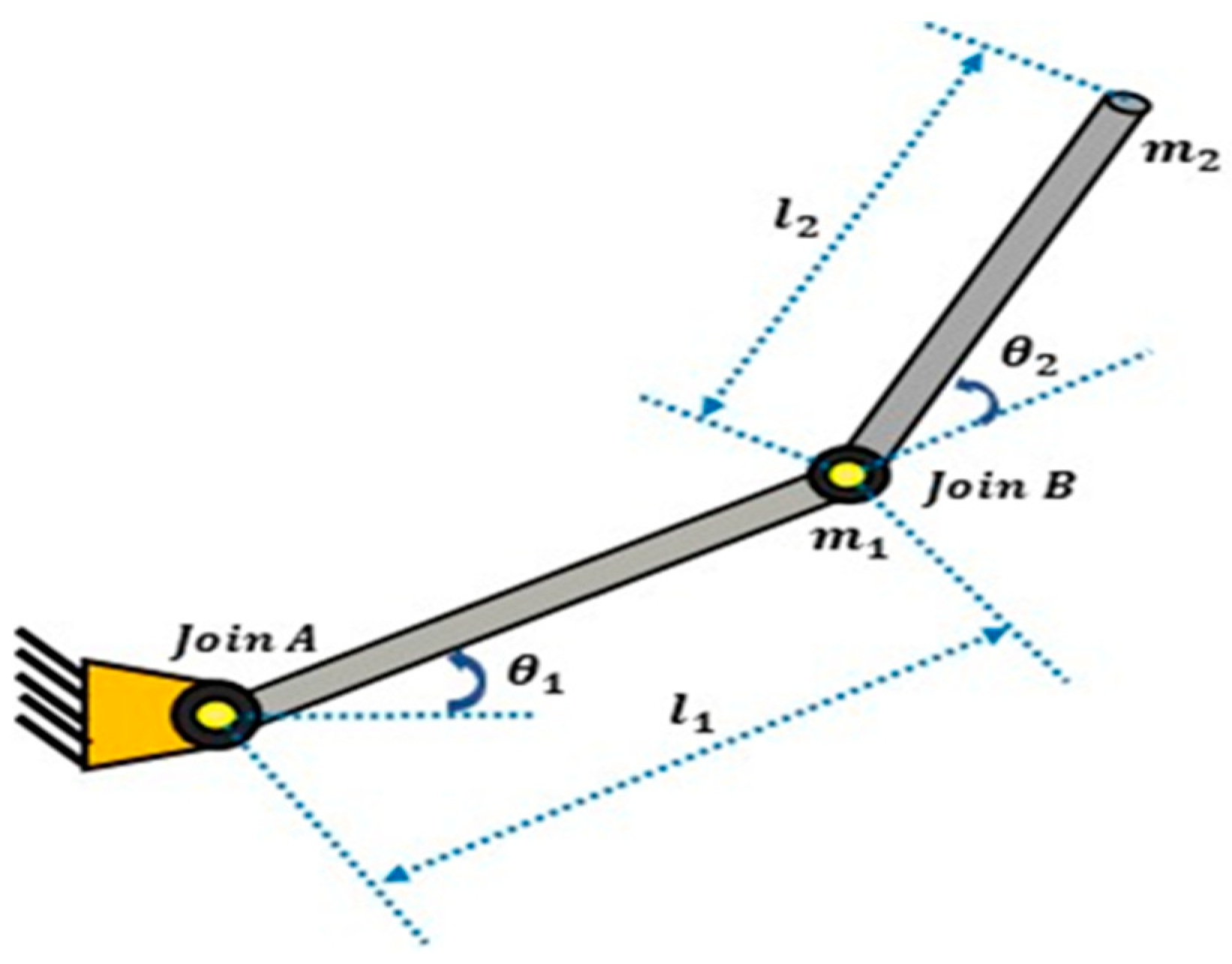
2. Dynamic Model of 2-LRRM

As shown in Figure 1, the 2-LRRM comprises two links with lengths ${\mathrm{l}}_1$ and ${\mathrm{l}}_2$, and their centre of masses is ${\mathrm{m}}_1$ and ${\mathrm{m}}_2$ respectively, which are determined at the distal ends of the links, to produce the control torque at joints A and B, DC motors will be utilized to predict the links angular positions ${\mathsf{\theta }}_{1 }$ and ${\mathsf{\theta }}_2$ and velocities ${\dot{\mathsf{\theta }}}_1$ and ${\dot{\mathsf{\theta }}}_2$, the encoders will be applied [18]. The dynamic equation of motion in robotics is utilized for setting up the equations of the controller. Actuators are used for the generation of the torque values that are necessary for the dynamic motion of the manipulator. The correlation between input torques and components configurations’ time change rates of the manipulator is concerned with deriving calculations of the manipulator motion due to the moments, and forces applied to it. As a consequence, the manipulator robot dynamic modelling contains the determination of functions that determine forces applying on structures, locations of the joint, velocities, and accelerations [19].

The x-position and y-position equations for ${\mathrm{m}}_1$ are expressed by:

$${ \mathrm{x}}_1={ \mathrm{l}}_1 \cos ({\mathsf{\theta }}_1)$$

(1)

$${ \mathrm{y}}_1={ \mathrm{l}}_1 \sin \left({\mathsf{\theta }}_1\right)$$

(2)

Likewise, the x position and y position equations of ${\mathrm{m}}_2$ are defined by

$${\mathrm{x}}_2={ \mathrm{l}}_1 \cos \left({\mathsf{\theta }}_1\right)+{ \mathrm{l}}_2 \cos \left({\mathsf{\theta }}_1+{\mathsf{\theta }}_2\right)$$

(3)

$${\mathrm{y}}_2={ \mathrm{l}}_1 \sin ({\mathsf{\theta }}_1)+{ \mathrm{l}}_2 \sin \left({\mathsf{\theta }}_1+{\mathsf{\theta }}_2\right)$$

(4)

The kinetic energy is written as:

$$\mathrm{KE}=\frac{1}{2}{\mathrm{m}}_1\left({\dot{\mathrm{x}}}_1^2+{\dot{\mathrm{y}}}_1^2\right)+\frac{1}{2}{ \mathrm{m}}_2 \left({\dot{\mathrm{x}}}_2^2+{\dot{\mathrm{y}}}_2^2\right)$$

(5)

And the potential energy can be given as:

$$\mathrm{PE}={ \mathrm{m}}_1{ \mathrm{g} \mathrm{l}}_1\sin \left({\mathsf{\theta }}_1\right)+{\mathrm{m}}_2 \mathrm{g}\left({\mathrm{l}}_{1 }\sin \left({\mathsf{\theta }}_1\right)+{\mathrm{l}}_2\sin \left({\mathsf{\theta }}_1+{\mathsf{\theta }}_2\right)\right)$$

(6)

Next, by Lagrange Dynamic, the Lagrangian form can be expressed as:

$$\mathrm{L}=\mathrm{KE}-\mathrm{PE}$$

(7)

The Euler-Lagrange Equation can be defined by:

$$\frac{\mathrm{d}}{\mathrm{dt}} \left[\frac{\partial \mathrm{L}}{\partial \dot{{\mathsf{\theta }}_{\mathrm{i}}}}\right]-\frac{\partial \mathrm{L}}{\partial {\mathsf{\theta }}_{\mathrm{i}}}={ \mathrm{F}\mathsf{\theta }}_{\mathrm{i}}$$

(8)

where, ${\mathrm{F}\mathsf{\theta }}_{\mathrm{i}}$ represents the torque on i’th link. Finally, according to the Lagrangian equation, the dynamics of the manipulator can be written as the two coupled nonlinear differential equations [20]:

$$\begin{gathered} {\mathsf{\tau }}_1=\left[\left({\mathrm{m}}_1+{\mathrm{m}}_2\right){\mathrm{l}}_1^2+{\mathrm{m}}_2{\mathrm{l}}_2^2+2{\mathrm{m}}_2{\mathrm{l}}_1{\mathrm{l}}_{2 }\cos \left({\mathsf{\theta }}_2)\right]{\ddot{\mathsf{\theta }}}_1+[{\mathrm{m}}_2{\mathrm{l}}_2^2+{\mathrm{m}}_2{\mathrm{l}}_1{\mathrm{l}}_2\cos \left({\mathsf{\theta }}_2\right)\right]{\ddot{\mathsf{\theta }}}_2 \\ \hspace{1em}\hspace{1em} -{\mathrm{m}}_2{\mathrm{l}}_1{\mathrm{l}}_2\left(2\dot{{\mathsf{\theta }}_1}\dot{{\mathsf{\theta }}_2}+{\dot{\mathsf{\theta }}}_2^2\right)\sin \left({\mathsf{\theta }}_2\right)+\left({\mathrm{m}}_1+{\mathrm{m}}_2\right){\mathrm{gl}}_1\cos \left({\mathsf{\theta }}_1\right)+{\mathrm{m}}_2{\mathrm{gl}}_2\cos \left({\mathsf{\theta }}_1+{\mathsf{\theta }}_2\right) \end{gathered}$$

(9)

$${ \mathsf{\tau }}_2=\left[{\mathrm{m}}_2{\mathrm{l}}_2^2+{\mathrm{m}}_2{\mathrm{l}}_1{\mathrm{l}}_2\cos ({\mathsf{\theta }}_2\right)]{\ddot{\mathsf{\theta }}}_1+{\mathrm{m}}_2{\mathrm{l}}_2^2{\ddot{\mathsf{\theta }}}_2+{\mathrm{m}}_2{\mathrm{l}}_1{\mathrm{l}}_2{\dot{\mathsf{\theta }}}_1^2\sin \left({\mathsf{\theta }}_2\right)+{\mathrm{m}}_2{\mathrm{gl}}_2\cos \left({\mathsf{\theta }}_1+{\mathsf{\theta }}_2\right)$$

(10)

The dynamics of this manipulator are represented in standard form

$$\mathrm{M}\left(\mathsf{\theta }\right)\ddot{\mathsf{\theta }}+\mathrm{V}\left(\mathsf{\theta },\dot{\mathsf{\theta }}\right)+\mathrm{g}\left(\mathsf{\theta }\right)=\mathsf{\tau }$$

(11)

With $\mathrm{V}\left(\mathsf{\theta },\dot{\mathsf{\theta }}\right)$ represents the Coriolis/centripetal vector, $\mathrm{M}\left(\mathsf{\theta }\right)$ represents the inertia matrix, and $\mathrm{g}\left(\mathsf{\theta }\right)$ equals the gravity vector. As can be noted that M(θ) is symmetric.

$$\mathrm{M}=\left[ \begin{array}{cc}\mathrm{M}11& \mathrm{M}12\\ \mathrm{M}21& \mathrm{M}22\end{array}\right]$$

(12)

$${\mathrm{M}}_{11}=\left({\mathrm{m}}_1+{\mathrm{m}}_2\right){\mathrm{l}}_1^2+{\mathrm{m}}_2{\mathrm{l}}_2^2+2{\mathrm{m}}_2{\mathrm{l}}_1{\mathrm{l}}_{2 }\cos \left({\mathsf{\theta }}_2\right)$$

(13)

$${\mathrm{M}}_{12}={\mathrm{m}}_2{\mathrm{l}}_2^2+{\mathrm{m}}_2{\mathrm{l}}_1{\mathrm{l}}_{2 }\cos \left({\theta }_2\right)$$

(14)

$${\mathrm{M}}_{12}{\mathrm{M}}_{21}\& {\mathrm{M}}_{22}{ \mathrm{m}}_2{\mathrm{l}}_2^2$$

(15)

V represents the Coriolis and centrifugal matrix, which can be expressed by

$$\mathrm{V}=\left[\begin{array}{c}{\mathrm{V}}_1\\ {\mathrm{V}}_2\end{array}\right]$$

(16)

$${\mathrm{V}}_1=-{\mathrm{m}}_2{\mathrm{l}}_1{\mathrm{l}}_2\left(2\dot{{\mathsf{\theta }}_1}\dot{{\mathsf{\theta }}_2}+{\dot{\mathsf{\theta }}}_2^2\right)\sin \left({\mathsf{\theta }}_2\right)$$

(17)

$${\mathrm{V}}_2={\mathrm{m}}_2{\mathrm{l}}_1{\mathrm{l}}_2{\dot{\mathsf{\theta }}}_1^2\sin \left({\mathsf{\theta }}_2\right)$$

(18)

The gravity vector $\mathrm{g}={[{ \mathrm{g}}_{12 }{\mathrm{g}}_{21 }]}^{\mathrm{T}}$ is given by:

$${\mathrm{g}}_{12}=\left({\mathrm{m}}_1+{\mathrm{m}}_2\right){\mathrm{gl}}_1\cos \left({\mathsf{\theta }}_1\right)+{\mathrm{m}}_2{\mathrm{gl}}_2\cos \left({\mathsf{\theta }}_1+{\mathsf{\theta }}_2\right)$$

(19)

$${\mathrm{g}}_{21}={ \mathrm{m}}_2{\mathrm{gl}}_2\cos \left({\theta }_1+{\theta }_2\right)$$

(20)

The nominal values of the parameters for the model are shown in

Table 1. The nominal parameters of 2-LRRM.

Parameters	Nominal Value
m1	0.1 kg
m2	0.1 kg
l1	0.8 m
l2	0.4 m
g	9.81 m/s2

[19].

3. Artificial Gorilla Troops Optimizer (GTO)

An optimization algorithm provides a smart solution to fix different problems because, in real life, the intelligence in the collective behavior of natural organisms has been studied and converted into simple and smart equations [21,22,23]. In this study, an artificial GTO is suggested for tuning the controller’s parameters. Gorilla animals arrange their lives as troops, and many adult females with their children with adult males with silver-coloured hair. They call him silverback gorilla. Each male and female try to go away from their place for another place. Males want to leave their places and be within another group by drawing females’ attention to a new troop, while others are still not leaving the same place from their birth and being in the same troop. When the leader dies, the populations available try to control others or handle the silverback to lead them. At this point, the chosen leader is considered the suitable choice, and all other males obey him and leave away from the worst choice. Two phases will describe this algorithm as indicated below [24,25].

3.1. Exploration Phase

In this phase, each one will be considered a competitor to the best decision from the silverback gorilla. Three decisions can be taken in this phase and are appeared in Equation (21), the first decision will increase the algorithm exploration by leaving to an undefined or unknown position, and the other one will make balance behaviour by leaving to a new group while the final choice will raise GTO capability for finding many positions regarded as a known ones.

$$\mathrm{GX}\left(\mathrm{t}+1\right)=\{\begin{array}{c}\left(\mathrm{UL}-\mathrm{LL}\right){\mathrm{r}}_1+\mathrm{LL}, \mathrm{if} \mathrm{rand} <\mathrm{P}\\ \left({\mathrm{r}}_2-\mathrm{a}\right){\mathrm{X}}_{\mathrm{r}}\left(\mathrm{t}\right)+\mathrm{L}\times \mathrm{H}, \mathrm{if} \mathrm{rand} \ge 0.5\\ \mathrm{X}\left(\mathrm{i}\right)-\mathrm{L}\left(\mathrm{L}\left(\mathrm{X}\left(\mathrm{t}\right)-{\mathrm{GX}}_{\mathrm{r}}\left(\mathrm{t}\right)\right)+{\mathrm{r}}_3\left(\mathrm{X}\left(\mathrm{t}\right)-{\mathrm{GX}}_{\mathrm{r}}\left(\mathrm{t}\right)\right)\right), \mathrm{if} \mathrm{rand} <0.5\end{array}$$

(21)

GX(t + 1) is a nominee in the next iteration. X_r (t) parameter is used for anyone in the troop nominees taken randomly from them and GX_r (t) will be the position of that random one. UL and LL are the upper and lower variables levels, ${\mathrm{r}}_1$, ${\mathrm{r}}_2$ and ${\mathrm{r}}_3$ are assumed to be random items [0] to [1]. The variables a, L and H is calculated below:

$$\mathrm{a}=\mathrm{C}\times \left(1-\mathrm{It}∕\mathrm{MaxIt}\right)$$

(22)

$$\mathrm{C}=\cos \left(2\times {\mathrm{r}}_4\right)+1$$

(23)

$$\mathrm{L}=\mathrm{c}\times \mathrm{l}$$

(24)

$$\mathrm{H}=\mathrm{Z}\times \mathrm{X}\left(\mathrm{t}\right)$$

(25)

$$\mathrm{Z}=\left[-{\mathrm{a} }_{,}\mathrm{a}\right],$$

(26)

3.2. Exploitation Phase

Two decisions will be taken in this phase. One decision is to obey the silverback gorilla, the leader, while the other is to be a competitor with the adult ones. Each decision is selected by comparing with the value calculated in Equation (26), if a ≥ W, the first decision is taken, while if a < W second decision will be taken. W is a predetermined parameter given before starting.

3.2.1. Following the Adult Silverback Leader

Gorilla: At this point, the silverback will be the leader, and others will follow his decisions to search their food places. It is taken if a ≥ w and shown clearly in the equation below:

$$\mathrm{GX}\left(\mathrm{t}+1\right)=\mathrm{L}\times \mathrm{M}\times \left( \mathrm{X}\left(\mathrm{t}\right)-{\mathrm{X}}_{\mathrm{silverback} }\right)+\mathrm{X}\left(\mathrm{t}\right)$$

(27)

${ \mathrm{X}}_{\mathrm{silverback} }$ is the leader’s place, and $\mathrm{X}\left(\mathrm{t}\right)$ is the gorilla location; the variables $\mathrm{L}$ and $\mathrm{M}$ are chosen.

3.2.2. Competition for Adult Females

In this case, the decision will take as young males have adulthood age; the struggle is severe when they attack each other to initiate new families with adult females. Decision now is taken when a < w as can be described clearly in the equation below:

$$\mathrm{GX}\left(\mathrm{i}\right)={\mathrm{X}}_{\mathrm{silverback} }-\left({\mathrm{X}}_{\mathrm{silverback} }\times \mathrm{R}- \mathrm{X}\left(\mathrm{t}\right)\times \mathrm{R}\right)\times \mathrm{A},$$

(28)

$$\mathrm{R}=2\times r_5-1,$$

(29)

$$\mathrm{A}=\mathsf{\beta }\times \mathrm{E},$$

(30)

$$\mathrm{E}=\left\{\begin{array}{c}{\mathrm{N}}_1=\mathrm{rand}\ge 0.5\\ {\mathrm{N}}_2=\mathrm{rand}<0.5\end{array}\right.$$

(31)

where “R” explain the impact force, which is found by solving Equation (23), r₅ is a value taken randomly between [0, 1] as struggle happens, Equation (26) was adopted to find the violence value during struggles, and A is the vector used for utilizing to solve the violence level by using Equation (24). Several parameters will be preset previously, like a, β, and E, which are regarded as an effect of violence on choice levels. The fitness function of all GX (t) is found, as the fitness function of GX (t) < X (t), the GX (t) will use the X (t) as an optimal solution, the best decision taken from the troop is taken as a new silverback leader. Figure 2 below explains all algorithm steps.

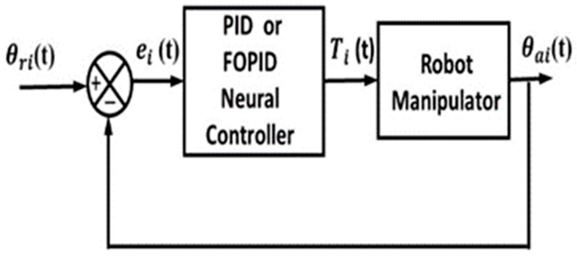
4. The Structures of the Proposed Controllers

In this section, we introduce details information about the structures of the proposed hybrid neural controllers. Here we consider the problem of controlling one variable or the system is of type a Single Input a Single Output (SISO) system. Therefore, the following control structures represent part of the controller unit in a Multi-Input Multi-Output (MIMO) system.

4.1. Conventional PID Controller (Con-PID)

PID controller is the major widely proposed prevalent controller. It consists of three actions: proportional action, integral action, and derivative action. The proportional action reduces the rise time of the response, while the Integral action improves steady-state error, and the derivative action reduces the overshoot and improves the stability margin [26,27]. Since the derivative term is sensitive to measurement noise, a filter is added to reduce the effect of measurement noise. The derivative term without a filter may amplify the noise signal in the controller output and causes loss of control. A typical PID controller transfer function with the filter is indicated in Equation (32).

$$G{\left(s\right)}_{PID}=K_p+K_i \frac{1}{\mathrm{s}}+ K_d\mathrm{s} \frac{N}{s+N}$$

(32)

The three gains $K_p$, $K_i$ and $K_d$ determine the effect of these proportional, integral, and derivative actions, respectively, and N is the filter’s corner frequency. Therefore, the gains $K_p$, $K_i$, $K_d$, and N parameters are needed to be tuned to realize a certain objective. The conventional PID controller structure with filter is shown in Figure 3, and the block diagram of the feedback control system with PID or FOPID controller is shown in Figure 4.

4.2. Conventional Fractional Order PID Controller (Con-FOPID)

This controller type is regarded as an enhanced scheme of a conventional PID controller because the values of order in the derivative and integral parts are fractional numbers instead of integer numbers [28,29]. These two fractional parameters are μ and λ; accordingly, due to these parameters and the N parameter of the filter, the controller needs to tune six parameters instead of four in case of using the filter. The additional tuned parameters will save robustness in the system’s behavior and improve the performance. The FOPID controller structure is shown in Figure 5, and the transfer function of the FOPID controller is shown in Equation (33).

$$G{\left(s\right)}_{FOPID}=K_p+K_i \frac{1}{{\mathrm{S}}^{ \mathsf{\lambda }}}+K_d{\mathrm{s}}^{\mu }\frac{N}{s+N}$$

(33)

The tuned parameters of the FOPID controller will be $\left(K_p, K_i,K_d, \lambda , \mu , N\right)$ [30]. If λ = μ = 1, a conventional PID is obtained, while if one is 1 and the other is 0, it will be a conventional PI controller (if λ = 1, μ = 0) or conventional PD controller (if λ = 0, μ = 1). There are numerous methods to implement fractional differentiation and integration [31,32,33]. Oustaloup’s recursive approximation filter is widely used to approximate the fractional order transfer function, which is used in this work [34]. The feedback control system with the FOPID controller is shown in Figure 5 [35].

4.3. Self-Tuning Neural Network PID Controller (STNN-PID)

The self-tuning neural network PID controller consists of two main parts: the first part is a feed-forward NN unit used for auto-tuning the parameters ($K_p$,$K_{i }, K_d$) of the PID controller, and the second part is the three operations (proportional, integral, and derivative) of the conventional PID controller applied to the error between the desired and the actual control variable to produce the control signal. The conventional PID controller receives the values of its three parameters from the neural network at each sampling time. Neural network training is occurred once at the design step according to a performance index then the neural network model still the same during the operation. The neural network model architecture will be fixed before training [36,37].

The structure of the neural network part of the controller is illustrated in Figure 6. The input layer consists of three input neurons as follows; ${\theta }_{ri}$ is the required angular position of ith link, ${\theta }_{ai}$ is the actual angular position of the ith link, and $e_i$ is the error between the required and actual angular position of the ith link. The hidden layer consists of ten neurons, each hidden neuron connected with all input neurons via a weight value for each connection [38]. The activation function $\mathrm{H}\left(\mathsf{\Sigma }\right)$ is applied to the sum of these three connections for each hidden neuron. The activation function is depicted in Equation (34).

$$H\left(\mathsf{\Sigma }\right)=\left(2-{\mathsf{\Sigma }}^2\right)·e^{-{\mathsf{\Sigma }}^2}$$

(34)

The output layer consists of three neurons connected to all ten hidden neurons via a weight value for each connection. The output of each output neuron is the sum of all its connections with hidden neurons. The output of each output neuron represents one parameter value of the PID controller and is fed to the conventional PID controller. It is necessary to mention here that the corner frequency parameter N of the filter is tuned offline like the neural network parameters and is not auto-tuning parameter. The equation of the conventional PID controller is shown in Equations (32) and (35)–(38). The feedback control system with a self-tuning PID controller is shown in Figure 7.

4.4. Self-Tuning Neural Network FOPID Controller (STNN-FOPID)

The self-tuning neural network FOPID controller also consists of two main parts. The first part is a feed-forward neural network with the following features; the input layer, the hidden layer, the connections between neurons, and the type of activation function are the same as those used in the STNN-PID controller. The only difference from the neural network used in STNN-PID is the output layer. This layer consists of five neurons instead of three because of the need for five parameters $(K_p, K_i,K_d, \mathsf{\lambda }, \mathsf{\mu }$) to tune the FOPID controller. In other words, the additional neurons in the output layer or additional auto-tuning parameters are needed to tune the fractional order parameters λ and μ of integration and differentiation, respectively while the parameter N of the filter is tuned offline with NN parameters. The structure of the STNN-FOPID controller is shown in Figure 8.

The second part is the three operations (proportional, fractional integral, and fractional derivative) of the FOPID controller applied to the error between the desired and the actual control variable to produce the control signal. The FOPID controller receives five parameters from the neural network at each sampling time. The equation of the FOPID controller is illustrated in Equations (33) and (35)–(39). The block diagram of the feedback control system with a self-tuning neural network STNN-FOPID controller is shown in Figure 9.

4.5. Neural Network PID Controller (NN-PID)

The structure of this proposed hybrid controller NN-PID is shown in Figure 10. where in conventional PID controller λ = 1 and μ = 1. The structure depicts that the input layer consists of one neuron. This neuron represents the error e(k) between the desired and actual output of the controlled variable. The first hidden layer consists of three neurons. The input-output functions of these neurons are chosen according to the PID control law, while the input to these nodes is the error e(k) multiplied by the weight of connection for each neuron. This selection makes those neurons represent the role of proportional, integral, and derivative (PID) operations on its input and the weights of connections represent the gains $(K_p$,$K_{i }, K_d$) as shown in Equations (35)–(39).

$$P\left(k\right)=K_p\times e\left(k\right)$$

(35)

$$sum\left(k\right)=sum\left(k-1\right)+h\times e\left(k\right)$$

(36)

where, $sum\left(k\right)=0$.

$$I\left(k\right)=K_i\times sum\left(k\right)$$

(37)

$$f\left(s\right)=\frac{N}{s+N} e\left(s\right)\hspace{1em}\hspace{1em}\hspace{1em}\mathrm{the} \mathrm{filter} \mathrm{of} \mathrm{derivative}$$

(38)

$$D\left(t\right)=K_d\times \frac{d}{dt}f\left(t\right) \mathit{or} D\left(k\right)=K_d\times \left(f\left(k\right)-f\left(k-1\right) \right)/h$$

(39)

where, $Sum$ is the accumulator of integral operation. $P\left(k\right)$, I$\left(k\right)$, and $D\left(k\right)$ are the outputs of the first hidden layer neurons, which are proportional, integral, and derivative operations of the error, $h$ is the step size of the simulation.

The second hidden layer of the hybrid neural network controller consists of three neurons. Each neuron receives all outputs of the first hidden layer via different connection weights. The sum of all inputs for each neuron is submitted to the activation function $H\left(\mathsf{\Sigma }\right)$. The output of each neuron represents the result of its activation function, plus its previous output as illustrated in Equations (40)–(41). The applied activation function is shown in Equation (42).

$$\left[\begin{array}{c}\sum {\left(k\right)}^{11} \\ \sum {\left(k\right)}^{12}\\ \sum {\left(k\right)}^{13} \end{array}\right]=\left[ \begin{array}{ccc}v11& v12& v13\\ v21 & v22& v23 \\ v31& v32& v33\end{array} \right]\left[\begin{array}{c}P\left(k\right)\\ I\left(k\right)\\ D\left(k\right)\end{array}\right]$$

(40)

$$\left[\begin{array}{c}{O}_1\left(k\right)\\ O_2\left(k\right)\\ O_3\left(k\right)\end{array}\right]=\left[\begin{array}{c} H\left(\sum {\left(k\right)}^{11}\right)\\ H\left(\sum {\left(k\right)}^{12}\right)\\ H \left(\sum {\left(k\right)}^{13}\right)\end{array} \right]+\left[\begin{array}{c}{\alpha }_1·O_1\left(k-1\right)\\ {\alpha }_2·O_2\left(k-1\right)\\ {\alpha }_3·O_3\left(k-1\right)\end{array}\right]$$

(41)

$$H\left(\Sigma \right)=\frac{4}{\left(1+e^{-\Sigma }\right)}-2$$

(42)

where, $\sum {\left(\mathrm{k}\right)}^{1i}$ is the sum of input connections to the ith neuron of the second layer and $O_i\left(k\right),$ the output of the ith neuron of the second layer. $v\mathrm{ij}$ and ${\alpha }_i$ are the weight parameters.

The third hidden layer consists of three neurons. Each one receives all neuron’s outputs of the second hidden layer via weight for each connection plus its previous output via connection weight plus the previous output of the output layer neuron via the connection weight. Equations (43) and (44) depict the output of the third hidden layer.

$$\left[\begin{array}{c}\sum {\left(k\right)}^{21} \\ \sum {\left(k\right)}^{22}\\ \sum {\left(k\right)}^{23} \end{array}\right]=\left[ \begin{array}{ccc}w11& w12& w13\\ w21 & w22& w23 \\ w31& w32& w33\end{array} \right]\left[\begin{array}{c}{O}_1\left(k\right)\\ O_2\left(k\right)\\ O_3\left(k\right)\end{array}\right]$$

(43)

$$\left[\begin{array}{c}{S}_1\left(k\right)\\ S_2\left(k\right)\\ S_3\left(k\right) \end{array}\right]=\left[\begin{array}{c}\sum {\left(k\right)}^{21} \\ \sum {\left(k\right)}^{22}\\ \sum {\left(k\right)}^{23} \end{array}\right]+\left[\begin{array}{c}{\beta }_1·S_1\left(k-1\right)\\ {\beta }_2·S_2\left(k-1\right)\\ {\beta }_3·S_3\left(k-1\right) \end{array}\right]+\left[\begin{array}{c}{\sigma }_1·T\left(k-1\right)\\ {\sigma }_2·T\left(k-1\right)\\ {\sigma }_3·T\left(k-1\right) \end{array}\right]$$

(44)

where, $\sum {\left(\mathrm{k}\right)}^{2i}$ is the sum of input connections to the ith third hidden layer neuron ${\mathrm{S}}_i\left(\mathrm{k}\right)$ is the output of this neuron, $w\mathrm{ij}$, ${\beta }_{i }$, ${\sigma }_i$ and are weight parameters. Finally, the output layer consists of one neuron, the inputs to this neuron are all outputs of the third hidden layer via weight values and its previous output, as shown in Equation (45).

$$\mathrm{T}\left(\mathrm{k}\right)=\mathrm{T}\left(\mathrm{k}-1\right)+{\mathrm{r}}_1·{ \mathrm{S}}_1\left(\mathrm{k}\right)+{\mathrm{r}}_2·{\mathrm{S}}_2\left(\mathrm{k}\right)+{\mathrm{r}}_3·{\mathrm{S}}_3\left(\mathrm{k}\right)$$

(45)

The result of the output layer neuron represents the control signal applied to the system. The structure of the feedback control system with a neural network PID controller is shown in Figure 11.

4.6. Neural Network FOPID controller (NN-FOPID)

This hybrid neural network controller has the same number of inputs, hidden, and output layers and the same number of neurons in each layer as the structure of the NN-PID controller. Moreover, the same activation function H(Σ) is also used. The only differences between NN-PID and NN-FOPID structures are the implementation of integration and differentiation operations. The NN-FOPID structure enables the integration and differentiation actions to be performed in fractional order, while the NN-PID performs these operations in integer order only. The three actions of the FOPID controller are shown in Equations (46)–(49). The feedback control system with the FOPID controller is shown in Figure 11.

$$P\left(t\right)=K_p\times e\left(t\right)$$

(46)

$$I\left(t\right)=K_{i }\times D^{-\mathsf{\lambda }} e_{\theta i}\left(t\right)$$

(47)

$$f\left(s\right)=\frac{N}{s+N} e\left(s\right)\hspace{1em}\hspace{1em}\hspace{1em}\mathrm{the} \mathrm{filter} \mathrm{of} \mathrm{derivative}$$

(48)

$$D\left(t\right)=K_{d }\times D^{\mathsf{\mu }} f\left(t\right)$$

(49)

5. Simulation Results

The 2-LRRM model with the proposed controllers and test tracks was performed using MATLAB programming. The performance and robustness of all proposed controllers in trajectory tracking are presented in this section. For each link, the trajectory to be tracked is computed so that the manipulator will be forced to follow it. The results are then used to evaluate the proposed controller based on the performance index value of each controller. In this work, the assessment of all proposed controllers’ performance is based on the sum of the ITSE for both link trajectories [36]. The optimal controller is based on the lowest value of ITSE, written by Equation (50).

$$\mathrm{ITSE}=\int \left(\mathrm{t}\times { \mathrm{e}}_1^2\left(\mathrm{t}\right)+\mathrm{t}\times {\mathrm{e}}_2^2\left(\mathrm{t}\right)\right)\mathrm{dt}$$

(50)

where $e_1\left(t\right)$ and $e_2\left(t\right)$ are the difference between the desired trajectory and the actual trajectory of the link1 and link2. The desired trajectories ${\theta }_{r1}$ and ${\theta }_{r2}$ of the link1 and link2 can be expressed by Equations (51) and (52), respectively, as follows:

$${\theta }_{r1}=\left\{\begin{array}{c}0.75 t^2-0.25 t^{3 } (0<t<2)\\ -1.53 t-1.125t^2+0.125t^3 (2<t<4)\end{array}\right\}$$

(51)

$${\theta }_{r2}=\left\{\begin{array}{c}1.5 t^2-0.5 t^3 (0<t<2)\\ 12-12 t+4.5 t^2-0.5 t^3 (2<t<4)\end{array}\right\}$$

(52)

Before showing the results of all proposed controllers, we noted from many experiments that tuning the proposed controllers according to minimize the ITSE in Equation (50) led, in most cases, chattering in control signals. To make the optimization algorithm exclude the solution with the high chattering in the control signal, we propose a new fitness function for the optimization algorithm to make the chattering under our control.

The classical objective function was presented in Equation (53);

(min) J = ITSE

(53)

where (min) means minimizing the integral time square error.

The new proposed objective is presented in Equation (54)

(min) J = ITSE + Uc × ρ

(54)

where, Uc is the number of times that the slope of the control signal changes its sign. If the system has more than one control signal, the number of slop sign changes for all control signals are collected. ρ is a small positive number chosen as ${10}^{-8}$ or ${10}^{-7}$.

The execution time in the simulation part took 4 sec., and the step size of the simulation took 1 ms. The tuning experiment used two initial positions (0.1745, 0.1745) and (−0.1745, −0.1745) for ${\theta }_1$ and ${\theta }_2$ respectively at the same time to assess the solution to increase the amount of learning. The nominal parameters of the 2-LRRM model are considered in the design stage of all proposed controllers.

The GTO is used for tuning the parameters of all proposed controllers regarding the tracking error between the 2-LRRM actual and desired trajectories. The proposed GTO setting is the following; the size of the population = 80, team size = 10, and iterations = 1000. In the last iteration, the optimal solution took as the result of GTO. The number of tuning parameters and their range in the search space used by the GTO algorithm to find the optimal set of parameters is shown in

Table 2. The number of design parameters and their search range for all proposed controllers.

Controller	Total Number of Controller Parameters	Range of PID Gains Kp, Ki, Kd	Corner Frequency of Derivative Filter N	Range of Fractional Parameters	All Other Parameters Range
Con-PID	8	−150 to 150	10 to 100	μ ≡ 1 λ ≡ 1	--------
Con-FOPID	12	−150 to 150	10 to 100	μ ≡ 0 to 2 λ ≡ 0 to 2	--------
STNN-PID	122	−150 to 150	10 to 100	μ ≡ 1 λ ≡ 1	V ≡ −5 to 5 W≡ −1 to 1
STNN-FOPID	162	−150 to 150	10 to 100	μ ≡ 0 to 2 λ ≡ 0 to 2	V ≡ −5 to 5 W≡ −1 to 1
NNPID	66	−150 to 150	------	μ ≡ 1 λ ≡ 1	−1 to 1
NNFOPID	70	−150 to 150	------	μ ≡ 0 to 2 λ ≡ 0 to 2	−1 to 1

.

The performance index (ITSE) value and the number of sign changes in all control signals when using the two initial positions above for all suggested controllers are shown in

Table 3. The ITSE of the Proposed Controllers for Nominal Plant.

Controller	ITSE	No. of Slop Sign Change in All Control Signals
Con-PID	3.729543 × 10−4	93
Con-FOPID	2.227023 × 10−4	47
STNN-PID	3.075515 × 10−4	91
STNN-FOPID	3.883774 × 10−4	45
NNPID	0.954084 × 10−4	85
NNFOPID	0.748071 × 10−4	94

. The result generally indicates that the ITSE values for the proposed controllers with fractional order integral and fractional order derivative actions are better than controllers with integer order integral and integer order derivative actions. This is because the fractional order of these operations increases the flexibility of the controller by increasing its tuning parameters. The result shows that the proposed hybrid neural network controller NN-FOPID structure has the best value of the $ITSE=0.748071\times {10}^{-4}$ compared with other proposed controllers.

Now, to illustrate more details about the behavior of the proposed controllers, the initial position (0.1745, 0.1745) is used to execute all proposed, designed controllers on the nominal system. The obtained results are shown in

Table 4. The performance of the proposed controllers when the initial position (0.1745, 0.1745) is used.

Controller Type	Link No.	Rise Time	Over Shoot %	Settling Time	ITSE ×10−4
Con-PID	L1	0.070	6.6	0.684	1.47752
	L2	0.012	5.95	0.188	0.64646
Con-FOPID	L1	0.074	3.27	0.584	1.30261
	L2	0.054	1.40	0.131	0.10037
STNN-PID	L1	0.069	6.14	0.594	1.12337
	L2	0.012	7.41	0.394	0.83790
STNN-FOPID	L1	0.081	4.40	6.430	1.25247
	L2	0.026	1.05	0.166	1.00217
NN-PID	L1	0.081	1.60	0.134	0.34509
	L2	0.042	2.84	0.103	0.07345
NN-FOPID	L1	0.076	1.80	0.123	0.31060
	L2	0.043	0.47	0.043	0.03249

.

Table 4 shows that the NN-FOPID controller has a good rise time, minimum overshoot, and minimum settling time, as well as minimum ITSE for link1 and link2. Conversely, the Con-PID controller has the maximum settling time and maximum overshoot and worse rise time and ITSE. In addition, the control actions $T_{1 }$ and $T_{2 }$ for the NN-FOPID controller has the least control efforts as well as the trajectory followed by the 2-LRRM end effector for the NN-FOPID controller is the closest to the required path. The tracking of the trajectories of ${\theta }_1$ and ${\theta }_{2 }$, the $T_1$ and $T_{2 }$ as well as the trajectory tracked by the 2-LRRM end-effector are demonstrated in Figure 12.

5.1. Robustness Tests

Now, in the following tests, we will check the robustness of all proposed controllers without retuning the gains of controllers to prove the capability and robustness of each controller.

5.1.1. Change Initial Position

To check the robustness of all proposed controllers, another primary position [0.15, 0.15] for [${\theta }_1$, ${\theta }_2$] took for testing the capability of all the proposed controllers to follow the 2-LRRM on the required trajectory.

The obtained results of the performance index values for all suggested controllers are shown in

Table 5. The ITSE of the proposed controllers based on initial position (0.15, 0.15).

Controller	ITSE
Con-PID	1.82669 × 10−4
Con-FOPID	1.17614 × 10−4
STNN-PID	1.61995 × 10−4
STNN-FOPID	27.3328 × 10−4
NN-PID	1.05251 × 10−4
NN-FOPID	0.24644 × 10−4

. The tracking of the trajectories of ${\theta }_1$ and ${\theta }_2$, by the end-effector of the 2-LRRM by altering the initial position for all suggested controllers are presented in Figure 13.

Despite changing the initial positions, the NN-FOPID controller still performs better than the rest, because there is an almost smaller overshoot in the trajectory response for ${\theta }_1$ and ${\theta }_2$ and the settling time is almost small. While the STNN-FOPID has the worst response because of the ${\theta }_1$ and ${\theta }_2$ responses have large overshoots and long settling times. Moreover, the trajectory followed by the 2-LRRM end effector for the NN-FOPID controller remains the closest to the required trajectory.

5.1.2. Disturbance Addition

The robustness test of the suggested controllers was performed by using the disturbance term [sin (50t), sin (50t)] to the control signal [$T_{1 }$, $T_2$] and selecting the initial position as [0, 0] to [${\theta }_1$, ${\theta }_2$]. The obtained results of ITSE values for all suggested controllers are demonstrated in

Table 6. The ITSE of the proposed controllers based on disturbances sin (50t) for each link and initial position (0.0, 0.0).

Controller	ITSE
Con-PID	5.54533 × 10−4
Con-FOPID	1.43023 × 10−4
STNN-PID	191.4245 × 10−4
STNN-FOPID	Unstable
NN-PID	2.1375 × 10−4
NN-FOPID	0.092827 × 10−4

. The tracking of the trajectories of ${\theta }_1$ and ${\theta }_2$ and the trajectory followed by the 2-LRRM end-effector based on adding disturbance of sin50t N-m in both links are illustrated in Figure 14. As observed, the NN-FOPID hybrid neural controller gives the smallest ITSE, and smallest overshoot. All trajectories are closest to the desired trajectories and are free of oscillations compared with other control structures. The STNN-FOPID loses control and stability, while STNN-PID gives the worst performance compared with other controllers. Therefore, we conclude that the NN-FOPID is better than others for disturbance rejection.

5.1.3. Parameters Variations

The parameter variations also examined the performance of all proposed controllers by increasing the masses of both links by 5% and selecting the initial position as [0, 0] to [${\theta }_1$, ${\theta }_2$]. The values of ITSE for all proposed controllers are presented in

Table 7. The ITSE of the proposed controllers when increasing both masses of two links by 5% & Initial position (0.0, 0.0).

Controller	ITSE
Con-PID	1.183509 × 10−4
Con-FOPID	0.691371 × 10−4
STNN-PID	0.743505 × 10−4
STNN-FOPID	Unstable
NN-PID	0.196180 × 10−4
NN-FOPID	0.005068 × 10−4

. The tracking trajectories of ${\theta }_1$ and ${\theta }_2$ by the 2-LRRM end-effector for all controllers is displayed in Figure 15.

From the figures below in Figure 15, it is clear that the trajectory tracking for ${\mathsf{\theta }}_1$ and ${ \mathsf{\theta }}_2$ of the NN-FOPID controller are closest to the required ${\theta }_{r1}$ and ${\theta }_{r2}$ compared with other controller structures. As a result, the trajectory followed by the 2-LRRM end-effector with parameter variations for the NN-FOPID controller is very close to the desired trajectory. Therefore, the NN-FOPID controller outperforms all other proposed controllers when the values of system parameters vary. The STNN-FOPID controller also fails in this test and loses control and stability.

5.1.4. All Previous Tests Together

The effect of adding disturbance and parameter variation and changing the initial positions together on the proposed controllers is illustrated by the results in

Table 8. The ITSE of the proposed controllers based on initial position (0.15, 0.15), adding disturbances sin (50t) for both links torques and increasing 5% in masses of both links.

Controller	ITSE
Con-PID	6.54278 × 10−4
Con-FOPID	2.09812 × 10−4
STNN-PID	Unstable
STNN-FOPID	Unstable
NN-PID	4.26462 × 10−4
NN-FOPID	0.447529 × 10−4

.

Figure 16 shows the trajectory tracking of theta1 and theta2 and the path tracked by the end-effector of the 2-LRRM and the $T_1$ and $T_{2 }$ for disturbance, parameter variation as well as changing the initial positions for all controllers.

From the results presented, it can be deduced that the fractional order PID controllers generally outperform the integer order PID controllers for parameter variation, disturbance addition, and initial position change and, therefore, more robust. The best controller among all proposed controllers is NN-FOPID because it passed all tests successfully and gives minimum ITSE in all tests and the best performance.

6. Conclusions

In this paper, six controllers are suggested for a 2-LRRM for trajectory tracking problems. These controllers combine the advantages of the PID controller and the neural network. Different control strategies of these combinations and other structures were proposed to strengthen the control capability. The fractional order of integration and differentiation used in the FOPID controller gives another dimension toward strengthening the capability of the hybrid controller. In addition, using a smart metaheuristic GTO algorithm for tuning controllers’ parameters integrates the design components of the controller. Two controllers, NN-PID and NN-FOPID, are superior to others in their responses for the nominal system model because they reflect their stability and fast-tracking facility to the desired response path. Then different tests were done to check system capability and robustness in facing the following effects. The first test suggested a change in the initial position of the two links, the second test was an addition of disturbance to the torque of each link, and the third test changed in values of the system parameters where the masses of the two links are changed. The fourth test is taken the previous changes together synchronic. The results show that the performance index ITSE of the NN-FOPID controller for all tests from first to fourth are 0.24644 × ${10}^{-4}$, 0.092827 × ${10}^{-4}$, 0.005068 × ${10}^{-4}$, 0.447529 × ${10}^{-4}$, respectively. These values are the smallest values of ITSE obtained from testing all proposed controllers and indicate at the same time the smallest overshoot and settling time in system response. The NN-FOPID controller is more robust and capable than other controller structures. The future work will suggest using other optimization techniques instead of using the GTO algorithm, such as the Snake Optimization Algorithm (SOA), Squarril Search Algorithm (SSA), and Differential Search Algorithm (DSA) for tuning the gains of the proposed controllers. The best-proposed controller can be implemented practically using all necessary hardware components, such as a real robot manipulator and sensors, such as a camera.

References

1. Raj, R.; Kos, A. A Comprehensive Study of Mobile Robot: History, Developments, Applications, and Future Research Perspectives. Appl. Sci. 2022, 12, 6951. [Google Scholar] [CrossRef]
2. Chen, Y.; Zhao, T.; Dian, S.; Zeng, X.; Wang, H. Balance Adjustment of Power-Line Inspection Robot Using General Type-2 Fractional Order Fuzzy PID Controller. Symmetry 2020, 12, 479. [Google Scholar] [CrossRef]
3. Yang, C.; Huang, D.; He, W.; Cheng, L. Neural control of robot Manipulators with trajectory tracking constraints and input saturation. IEEE Trans. Neural Netw. Learn. Syst. 2021, 32, 4231–4242. [Google Scholar] [CrossRef] [PubMed]
4. Rishag, H.T.; Hameed, S.M. Improvement the DFIG active power with variable speed wind using particle swarm optimization. Diyala J. Eng. Sci. 2016, 9, 12–22. [Google Scholar] [CrossRef]
5. Elsisi, M.; Mahmud, K.; Lehtonen, M.; Darwish, M.M.F. An Improved Neural Network Algorithm to Efficiently Track Various Trajectories of Robot Manipulator Arms. IEEE Access 2021, 9, 11911–11920. [Google Scholar] [CrossRef]
6. Manjeet, M.; Sathans, S. Fuzzy based Control of Two Link Robotic Manipulator and Comparative Analysis. In Proceedings of the 2013 International Conference on Communication Systems and Network Technologies, Washington, DC, USA, 6–8 April 2013; IEEE: Piscataway Township, NJ, USA, 2013; pp. 562–567. [Google Scholar]
7. Dachang, Z.; Baolin, D.; Puchen, Z.; Shouyan, C. Constant Force PID Control for Robotic Manipulator Based on Fuzzy Neural Network Algorithm. Complexity 2020, 2020, 3491845. [Google Scholar] [CrossRef]
8. Rahali, H.; Zeghlache, S.; Benyettou, L. Fault-Tolerant Control of Robot Manipulators Based on Adaptive Fuzzy Type-2 Backstepping in Attendance of Payload Variation. Int. J. Intell. Eng. Syst. 2021, 14, 312–325. [Google Scholar] [CrossRef]
9. Mohan, V.; Chhabra, H.; Rani, A.; Singh, V. An expert 2DOF fractional order fuzzy PID controller for nonlinear systems. Neural Comput. Appl. 2018, 31, 4253–4270. [Google Scholar] [CrossRef]
10. Bingi, K.; Rajanarayan Prusty, B.; Pal Singh, A. A Review on Fractional-Order Modelling and Control of Robotic Manipulators. Fractal Fract. 2023, 7, 77. [Google Scholar] [CrossRef]
11. Sareena, A.; Rikesh, P. Application of PID Controller and Nonlinear Sliding Mode Control on Two Link Robotic Manipulator. Int. J. Eng. Res. Technol. 2019, 8, 504–508. [Google Scholar]
12. Elkhateeb, N.; Badr, R.I. Novel PID Tracking Controller for 2DOF Robotic Manipulator System based on Artificial Bee Colony Algorithm. Electr. Control. Commun. Eng. 2017, 13, 55–62. [Google Scholar] [CrossRef]
13. Ghamari, S.M.; Narm, H.G.; Mollaee, H. Fractional-order fuzzy PID controller design on buck converter with antlion optimization algorithm. IET Control. Theory Appl. 2022, 16, 340–352. [Google Scholar] [CrossRef]
14. Suid, M.H.; Ahmad, M.A. Optimal tuning of sigmoid PID controller using Nonlinear Sine Cosine Algorithm for the Automatic Voltage Regulator system. ISA Trans. 2022, 128, 265–286. [Google Scholar] [CrossRef]
15. Noordin, A.; Mohd Basri, M.A.; Mohamed, Z. Position and Attitude Tracking of MAV Quadrotor Using SMC-Based Adaptive PID Controller. Drones 2022, 6, 263. [Google Scholar] [CrossRef]
16. Cao, G.; Zhao, X.; Ye, C.; Yu, S.; Li, B.; Jiang, C. Fuzzy adaptive PID control method for multi-mecanum-wheeled mobile robot. J. Mech. Sci. Technol. 2022, 36, 2019–2029. [Google Scholar] [CrossRef]
17. Ghazali, M.R.B.; Ahmad, M.A.B.; Raja Ismail, R.M.T.B. Adaptive safe experimentation dynamics for data-driven neuroendocrine-PID control of MIMO systems. IETE J. Res. 2022, 68, 1611–1624. [Google Scholar] [CrossRef]
18. Bandyopadhyay, B.; Kamal, S. Stabilization and Control of Fractional Order Systems: A Sliding Mode Approach; Springer International Publishing: Cham, Switzerland, 2015; Volume 317. [Google Scholar] [CrossRef]
19. Almasri, E.; Uyguroglu, M.K. Modeling and Trajectory Planning Optimization for the Symmetrical Multiwheeled Omnidirectional Mobile Robot. Symmetry 2021, 13, 1033. [Google Scholar] [CrossRef]
20. Jothi, G.; Inbarani, H.H.; Azar, A.T.; Devi, K.R. Rough set theory with Jaya optimization for acute lymphoblastic leukemia classification. Neural Comput. Appl. 2019, 31, 5175–5194. [Google Scholar] [CrossRef]
21. Inbarani, H.H.; Banu, P.K.N.; Azar, A.T. Feature selection using swarm-based relative reduct technique for fetal heart rate. Neural Comput. Appl. 2014, 25, 793–806. [Google Scholar] [CrossRef]
22. Meghni, B.; Dib, D.; Azar, A.T.; Saadoun, A. Effective Supervisory Controller to Extend Optimal Energy Management in Hybrid Wind Turbine under Energy and Reliability Constraints. Int. J. Dyn. Control. 2018, 6, 369–383. [Google Scholar] [CrossRef]
23. Abdollahzadeh, B.; Soleimanian Gharehchopogh, F.; Mirjalili, S. Artificial gorilla troops optimizer: A new nature-inspired metaheuristic algorithm for global optimization problems. Int. J. Intell. Syst. 2021, 36, 5887–5958. [Google Scholar] [CrossRef]
24. Ginidi, A.; Ghoneim, S.M.; Elsayed, A.; El-Sehiemy, R.; Shaheen, A.; El-Fergany, A. Gorilla Troops Optimizer for Electrically Based Single and Double-Diode Models of Solar Photovoltaic Systems. Sustainability 2021, 13, 9459. [Google Scholar] [CrossRef]
25. Vázquez-Aveledo, S.; Romero, R.J.; Montiel-González, M.; Cerezo, J. Control Strategy Based on Artificial Intelligence for a Double-Stage Absorption Heat Transformer. Processes 2023, 11, 1632. [Google Scholar] [CrossRef]
26. Mosaad, A.M.; Attia, M.A.; Abdelaziz, A.Y. Whale optimization algorithm to tune PID and PIDA controllers on AVR system. Ain Shams Eng. J. 2019, 10, 755–767. [Google Scholar] [CrossRef]
27. Abdulameer, H.I.; Mohamed, M.J. Fractional Order Fuzzy PID Controller Design for 2-Link Rigid Robot Manipulator. Int. J. Intell. Eng. Syst. 2022, 15, 103–117. [Google Scholar]
28. Delavari, H.; Ghaderi, R.; Ranjbar, N.A.; HosseinNia, S.H.; Momani, S. Adaptive Fractional PID Controller for Robot Manipulator. arXiv 2010, arXiv:1206.20272010. [Google Scholar]
29. Meghni, B.; Dib, D.; Azar, A.T.; Ghoudelbourk, S.; Saadoun, A. Robust Adaptive Supervisory Fractional order Controller For optimal Energy Management in Wind Turbine with Battery Storage. Stud. Comput. Intell. 2017, 688, 165–202. [Google Scholar]
30. Micev, M.; Calasan, M.; Oliva, D. Fractional Order PID Controller Design for an AVR System Using Chaotic Yellow Saddle Goatfish Algorithm. Mathematics 2020, 8, 1182. [Google Scholar] [CrossRef]
31. Alzabut, J.; Tyagi, S.; Abbas, S. Discrete Fractional? Order BAM Neural Networks with Leakage Delay: Existence and Stability Results. Asian J. Control. 2022, 22, 143–155. [Google Scholar] [CrossRef]
32. Thaiprayoon, C.; Sudsutad, W.; Alzabut, J.; Etemad, S.; Rezapour, S. On the qualitative analysis of the fractional boundary value problem describing thermostat control model via ψ-Hilfer fractional operator. Adv. Differ. Equ. 2021, 2021, 201. [Google Scholar] [CrossRef]
33. Alzabut, J.; Abdeljawad, T. On existence of a globally attractive periodic solution of impulsive delay logarithmic population model. Appl. Math. Comput. 2008, 198, 463–469. [Google Scholar] [CrossRef]
34. Wiora, J.; Wiora, A. Influence of Methods Approximating Fractional-Order Differentiation on the Output Signal Illustrated by Three Variants of Oustaloup Filter. Symmetry 2020, 12, 1898. [Google Scholar] [CrossRef]
35. Patel, R.; Kumar, V. Multilayer Neuro PID Controller based on back propagation algorithm. Procedia Comput. Sci. 2015, 54, 207–214. [Google Scholar] [CrossRef]
36. Chertovskikh, P.A.; Seredkin, A.V.; Gobyzov, O.A.; Styuf, A.S.; Pashkevich, M.G.; Tokarev, M.P. An Adaptive PID Controller with an Online Auto-Tuning by a Pretrained Neural Network. J. Phys. Conf. Ser. 2019, 1359, 012090. [Google Scholar] [CrossRef]
37. Roy, R.; Tu, Y.-P.; Sheu, L.-J.; Chieng, W.-H.; Tang, L.-C.; Ismail, H. Path Planning and Motion Control of Indoor Mobile Robot under Exploration-Based SLAM (e-SLAM). Sensors 2023, 23, 3606. [Google Scholar] [CrossRef] [PubMed]
38. Ali, O.A.M.; El-Zoghby, H.M.; Ghany, A.G.M.A. Maximizing the Generated Power from Hybrid Wind-Solar System Based on Fuzzy Self Tuning Single Neuron PID Controller. In Proceedings of the 2018 Twentieth International Middle East Power Systems Conference (MEPCON), Cairo, Egypt, 18–20 December 2018; IEEE: Piscataway Township, NJ, USA, 2018; pp. 748–753. [Google Scholar] [CrossRef]
Figure 1. The 2-LRRM structure.
Fractalfract 07 00693 g001
Figure 2. GTO algorithm steps [21].
Fractalfract 07 00693 g002
Figure 3. Conventional PID controller structure with filter.
Fractalfract 07 00693 g003
Figure 4. The block diagram of the control system with Conventional. PID or FOPID controller structures.
Fractalfract 07 00693 g004
Figure 5. Con-FOPID controller structure.
Fractalfract 07 00693 g005
Figure 6. Self-tuning neural network PID controller.
Fractalfract 07 00693 g006
Figure 7. Feedback control system with self-tuning neural network PID controller.
Fractalfract 07 00693 g007
Figure 8. Self-tuning neural network FOPID controller.
Fractalfract 07 00693 g008
Figure 9. Feedback control system with self-tuning neural network FOPID controller.
Fractalfract 07 00693 g009
Figure 10. The structure of the NNPID controller.
Fractalfract 07 00693 g010
Figure 11. Block diagram of the feedback control system with neural network PID or FOPID controller.
Fractalfract 07 00693 g011
Figure 12. (a) Desired and actual   θ 1   , (b) Desired and actual   θ 2   , (c) Torque   T 1   , (d) Torque   T 2   , (e) Desired and actual paths of end-effector.
Fractalfract 07 00693 g012
Figure 13. Desired and actual trajectories (a) for   θ 1   , (b) for   θ 2   , (c) Desired and actual paths of end-effector based on initial positions (0.15, 0.15).
Fractalfract 07 00693 g013
Figure 14. Desired and actual trajectories (a) for   θ 1   , (b) for θ 2   , (c) Desired and actual paths of end-effector with disturbance term [sin (50t), sin (50t)] and the initial position (0, 0).
Fractalfract 07 00693 g014
Figure 15. Desired and actual trajectories (a) for θ 1   , (b) for   θ 2 , and (c) Desired and actual paths of end-effector for 5% increasing in both masses and initial position (0, 0).
Fractalfract 07 00693 g015
Figure 16. Desired and actual (a) for θ 1 , (b) for   θ 2 , (c) performance of all controllers for Torque   T 1   (d) performance of all controllers for Torque   T 2   , and (e) Desired and actual paths of end-effector when using initial position (0.15, 0.15), adding disturbance sin (50t) for both links torques and increasing 5% in masses of both links.
Fractalfract 07 00693 g016