Abstract
The Katz fractal dimension (KFD) is an effective nonlinear dynamic metric that characterizes the complexity of time series by calculating the distance between two consecutive points and has seen widespread applications across numerous fields. However, KFD is limited to depicting the complexity of information from a single scale and ignores the information buried under different scales. To tackle this limitation, we proposed the variable-step multiscale KFD (VSMKFD) by introducing a variable-step multiscale process in KFD. The proposed VSMKFD overcomes the disadvantage that the traditional coarse-grained process will shorten the length of the time series by varying the step size to obtain more sub-series, thus fully reflecting the complexity of information. Three simulated experimental results show that the VSMKFD is the most sensitive to the frequency changes of a chirp signal and has the best classification effect on noise signals and chaotic signals. Moreover, the VSMKFD outperforms five other commonly used nonlinear dynamic metrics for ship-radiated noise classification from two different databases: the National Park Service and DeepShip.
1. Introduction
The classification and identification of underwater acoustic targets are important in the fields of marine resource exploitation and national defense [1,2]. Among them, effective ship target recognition technology is pivotal for rights protection cruises and monitoring of infringing vessels in sensitive territories. And the recognition of ship-radiated noise (SRN) is undoubtedly the core of ship target recognition since it contains a huge number of characteristics, such as course angle, category, and speed [3,4]. However, SRN has non-Gaussian, nonlinear, and nonstationary characteristics [5,6,7], and the commonly used time-frequency domain metrics have difficulty effectively reflecting its nonlinear behavior. As a result, it has become clear that many researchers are focusing on the study of nonlinear dynamic metrics [8,9,10]. Among these, entropy, Lempel–Ziv complexity (LZC) [11], and fractal dimension-based nonlinear dynamic metrics emerge as prevalent and effective methodologies.
Entropy-based nonlinear dynamic metrics can quantitatively characterize the irregularity and uncertainty of the system [12]. The entropy theory was derived from information entropy. With the gradual deepening of the study of entropy theory, various entropies have been proposed, such as sample entropy (SE) [13], fuzzy entropy (FE) [14], permutation entropy (PE) [15], and dispersion entropy (DE) [16]. However, each of these entropy metrics has its own unique limitations. For instance, SE measures the dynamic complexity of a time series by calculating the rate at which new patterns emerge, but is slow and lacks stability when calculating longer time series. FE improves stability over SE but still has poor computational efficiency. Although PE enhances computational efficiency substantially, it considers only the sequence order of amplitudes, disregarding the amplitude information of the signal. While DE accounts for amplitude information, it lacks robustness against noise interference.
LZC, a prevalent nonlinear dynamic metric, is routinely employed to evaluate the level of disorder present in time series [11]. However, since the LZC utilizes binary mapping, this results in the loss of valid information about the original signals [17]. In 2002, Bai et al. proposed permutation LZC (PLZC) by substituting binary mapping for permutation patterns, which is more efficient and robust in EGG analysis [18]. Unfortunately, PLZC still suffers from the loss of the amplitude information. To tackle this problem, Mao et al. developed dispersion LZC (DLZC) by combining the normal cumulative distribution function (NCDF) in DE, and the experimental result shows that it can effectively follow the dynamic changes in heart rate time series [19]. However, the separability of DLZC is not prominent when used as a separate feature. To address this issue, dispersion entropy-based LZC (DELZC) [20] and fluctuation-based DLZC (FDLZC) [21] are proposed by improving the mapping method to enhance the separability of DLZC.
Similar to the concepts of entropy and LZC, the fractal dimension can characterize extraordinarily complex objects, including those that are non-smooth, irregular, and fragmented. In 1988, inspired by the Mendelbrot fractal dimension [22], Katz proposed a method for calculating fractal dimension based on waveform data named Katz fractal dimension (KFD) [23], which has been widely concerned, especially in the field of biomedicine. In addition, some researchers have proposed many other fractal dimension-based nonlinear dynamic metrics, such as the box fractal dimension (BFD) [24], Higuchi fractal dimension (HFD) [25], correlation dimension [26], and Hausdorff dimension [27] to analyze the irregular time series. Among these metrics, KFD, BFD, and HFD are more frequently utilized, with KFD being the most computationally efficient and without parameters to be set [28].
However, the nonlinear dynamic metrics described above only reflect the complexity of the time series at single scale, which leads to the loss of important information at remaining scales. Afterwards, some researchers proposed multiscale-based nonlinear dynamic metrics. Humeau–Heurtier [29] proposed multiscale entropy to quantify the complexity of time series. However, this traditional multiscale process leads to shorter lengths of coarse-grained series when the scale factor is increased, which, in turn, makes the stability decrease. To address this flaw, a refined composite multiscale process was proposed by changing the altering sampling point of the sub-series [30]. Li et al. [31] first applied the refined composite multiscale process to fractal dimensions in 2023, presenting the hierarchical refined composite multiscale fractal dimension, which represents exceptional performance in feature extraction of SRN. Nevertheless, the refined composite multiscale process still has the disadvantage of significantly shortening the length of coarse-grained series when the scale factor is large, which leads to a decrease in accuracy. In response to the above issues, Su et al. [32] developed a variable-step multiscale process and combined it with LZC in 2022. The variable-step multiscale process improves the coarse-grained process, reveals more potential information, and achieves a higher and more robust complexity.
In response to the inability of KFD to reflect potential information at different scales and the problem that the traditional multiscale process suffers from the loss of signal sub-series information as the time series scale increases, we proposed a novel fractal dimension algorithm, termed the variable-step multiscale Katz fractal dimension (VSMKFD). The main contributions and innovations of this paper are as follows: (1) a VSMKFD is proposed that adopts the variable-step multiscale process to optimize and improve the traditional multiscale process; (2) three classical simulated experiments are carried out to showcase the diverse capabilities of the VSMKFD, and the efficacy of the proposed method is validated through two SNR cases.
The structure of this article is organized as follows: Section 2 presents the fundamental definition of the KFD and introduces the proposed VSMKFD. Section 3 demonstrates the capability of VSMKFD based on three simulated experiments. Section 4 evaluates the application of VSMKFD in the SRN through two cases. Section 5 concludes the article.
2. Methodology
2.1. KFD
The fractal dimension is a popular physical quantity that quantitatively characterizes the complexity of a time series. KFD has been widely used in the field of nonlinear dynamics due to its computationally efficient advantages. The computational procedures of KFD are as follows:
Step 1: For a time-series , calculate the length of the series, which defined as :
Step 2: The maximum distance between the 1st point and th point is calculated according to Equation (2):
Step 3: The KFD can be calculated as expressed in the following equation:
2.2. VSMKFD
The KFD can only characterize the complexity of a time series on a single scale. Therefore, it is difficult to fully respond to the effective information in the time series. In order to more accurately depict the complexity of a time series, we introduced a variable-step multiscale process into the KFD and then proposed the VSMKFD. The specific steps of the VSMKFD are as follows:
Step 1: A given time series is converted into several new sub-series by the following variable-step multiscale process:
where and represent the step size and scale factor, respectively, and is the th element of the th variable-step multiscale coarse-grained series.
Step 2: The KFD for all the sub-series obtained in Step 1 are calculated, and the mean value of KFD of all sub-series is defined as the VSMKFD:
To understand the variable-step multiscale process more intuitively, we take the as an example, and Figure 1 displays the schematic diagram of the traditional multiscale process and variable-step multiscale process. From Figure 1, it can be seen that when , only one series is obtained in the traditional multiscale process, but in the variable-step multiscale process, three different sub-series can be obtained, which can mine more potential information from the time series. Therefore, the variable-step multiscale process can reflect the complexity of the original time series more comprehensively.
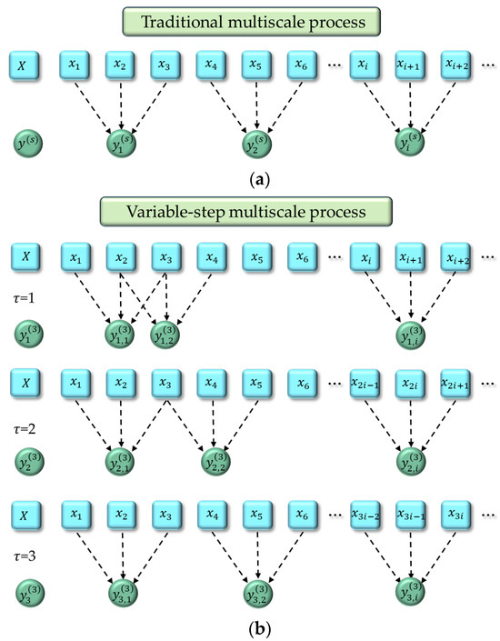
Figure 1.
The schematic diagram of multiscale process (): (a) traditional multiscale process; (b) variable-step multiscale process.
3. The Simulated Signal Analysis
In this section, we showcase the unique properties of the proposed VSMKFD through three classic simulated experiments and compare its performance with five other variable-step multiscale-based nonlinear dynamic metrics, including variable-step multiscale HFD (VSMHFD), variable-step multiscale BFD (VSMBFD), variable-step multiscale DE (VSMDE), variable-step multiscale PE (VSMPE), and variable-step multiscale LZC (VSMLZC). VSMKFD, VSMBFD, and VSMLZC do not relate the selection of parameters; the embedding dimension and time delay of VSMPE are 3 and 1, respectively; the of VSMHFD is set to 20, and the category number of VSMDE is 6.
3.1. The Chirp Signal Experiment
The chirp signal is known for its frequency variation over time, making it an apt choice for such experiments, and the chirp signal is defined as follows:
where is the modulation frequency, taken as 1.5; is called the initiation frequency, taken as 10 Hz; the time duration is 16 s; the sampling frequency is 1000 Hz, and its frequency is increased from 10 Hz to 40 Hz.
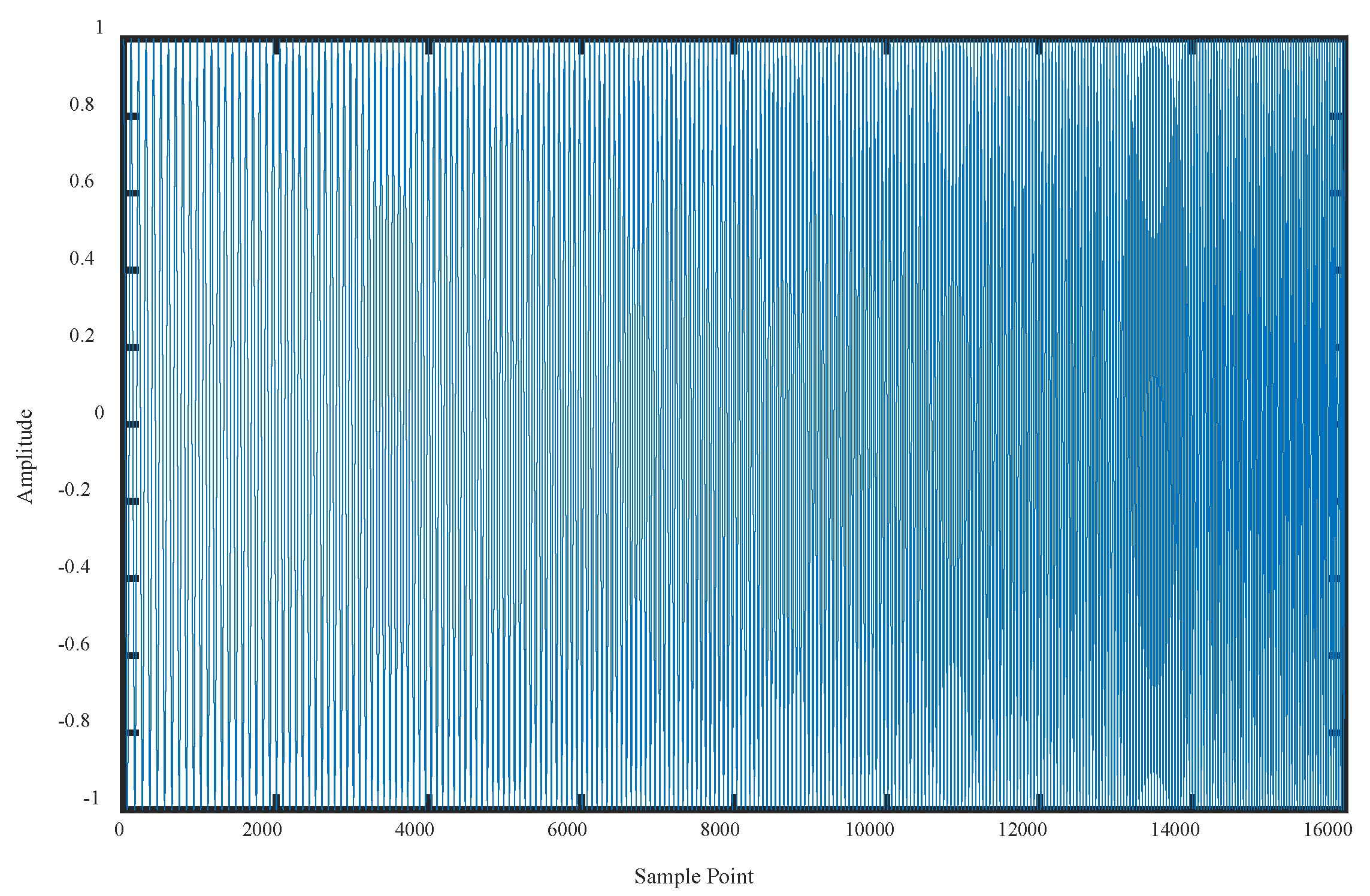
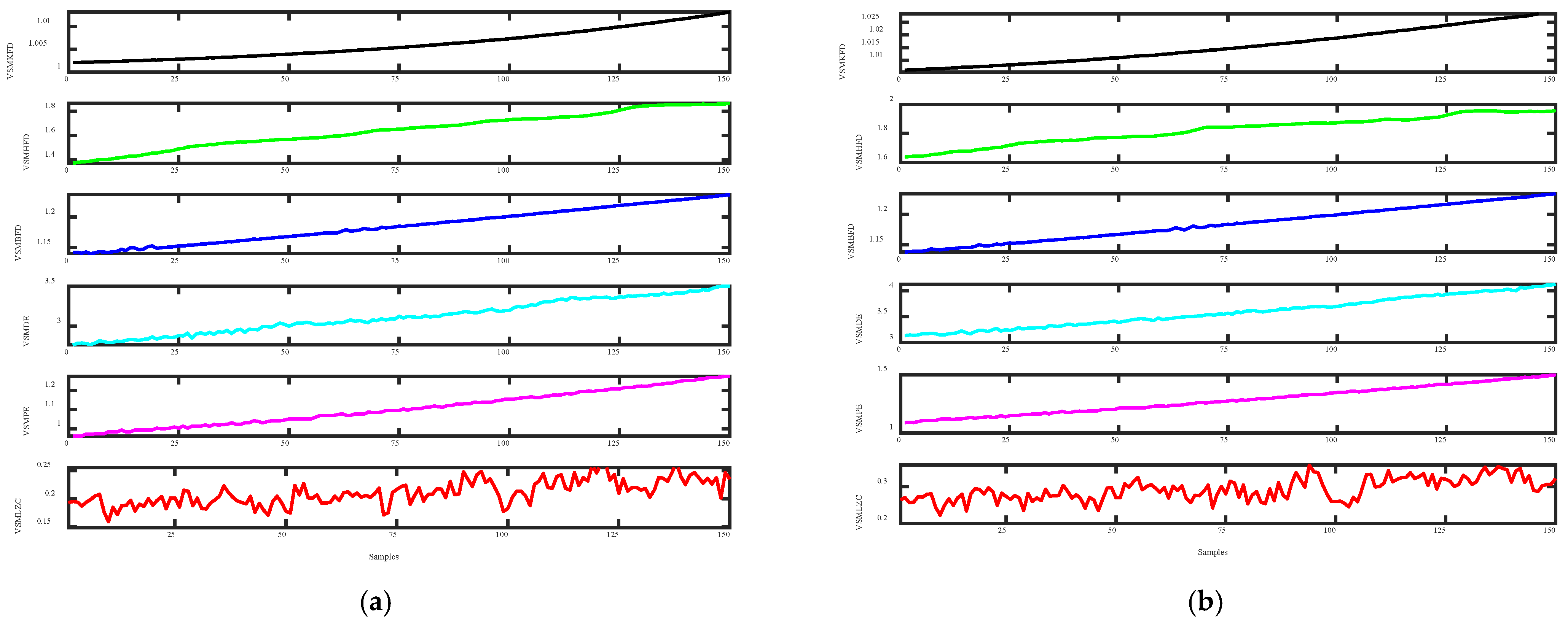
Figure 2 displays the waveform of the chirp signal. It encompasses a total of 16,000 sample points, the sliding window of 1 s is chosen, with a 90% overlap of this window, which allows us to obtain 150 samples. And the complexity curves of six metrics for the chirp signal are presented in Figure 3, where we only present the situations of and .
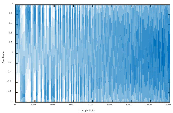
Figure 2.
The waveform of chirp signal.
Figure 3.
The complexity curves of six metrics for chirp signal: (a) ; (b) .
As exhibited in Figure 3, whether or , the complexity curves of six nonlinear dynamic metrics present an upward trend, reflecting the gradual enhancement of chirp signal frequency; among them, except for VSMKFD and VSMHFD, the curves of the remaining four metrics fluctuated to varying degrees, with the most severe fluctuations in VSMLZC; and the complexity curve of VSMKFD is much smoother than the VSMHFD curve. From the above analysis, we can observe that VSMKFD is able to more effectively reflect the changes in frequency than other nonlinear dynamic metrics.
3.2. The Noise Signal Classification Experiment
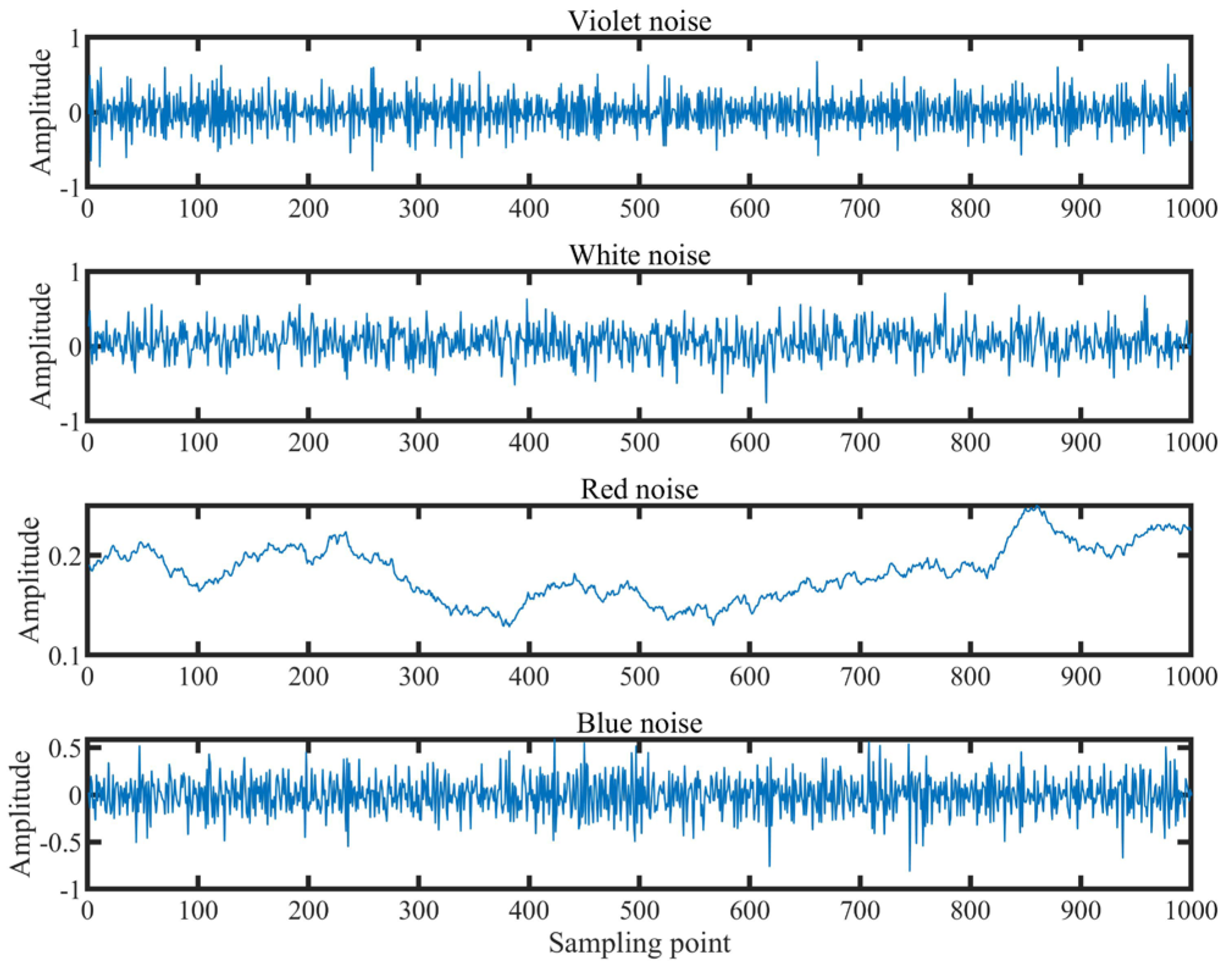
For this classification experiment, four distinct noise signals were selected to illustrate the superior performance of the proposed VSMKFD, consisting of violet noise, white noise, red noise, and blue noise. Then we take 100 non-overlapping samples, each with a total of 1000 sampling points. Figure 4 shows the waveforms of four noise signals under one sample to display the characteristics of these noise signals.

Figure 4.
The waveforms of four noise signals.
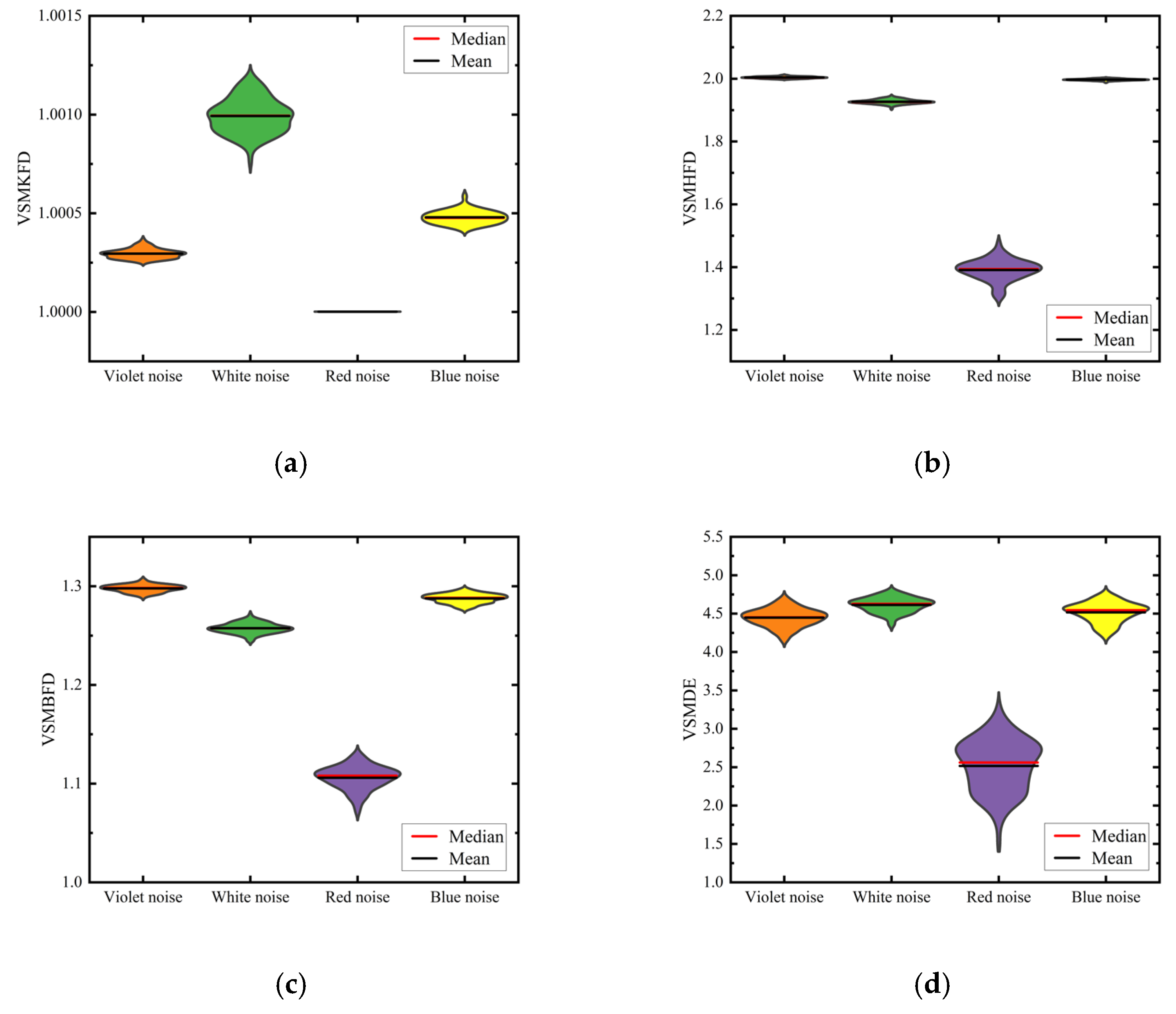
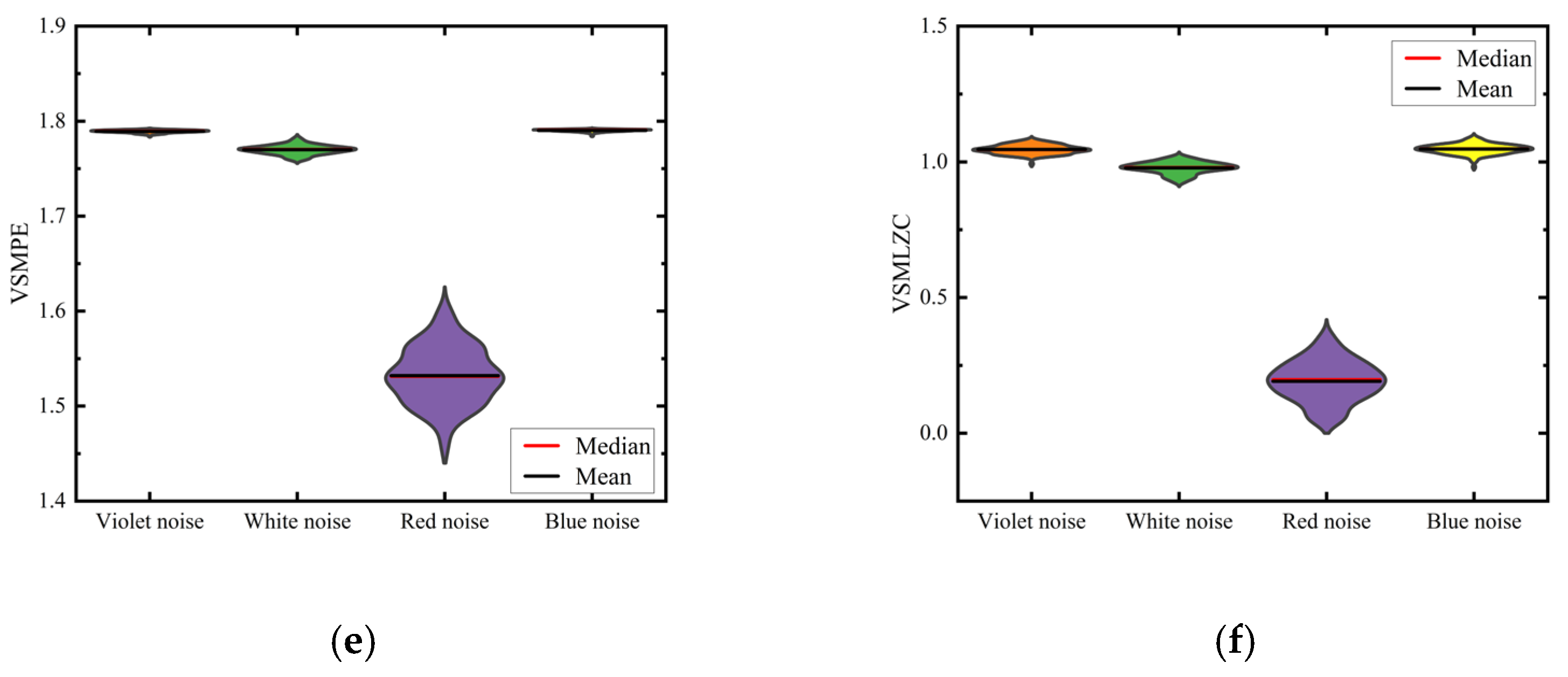
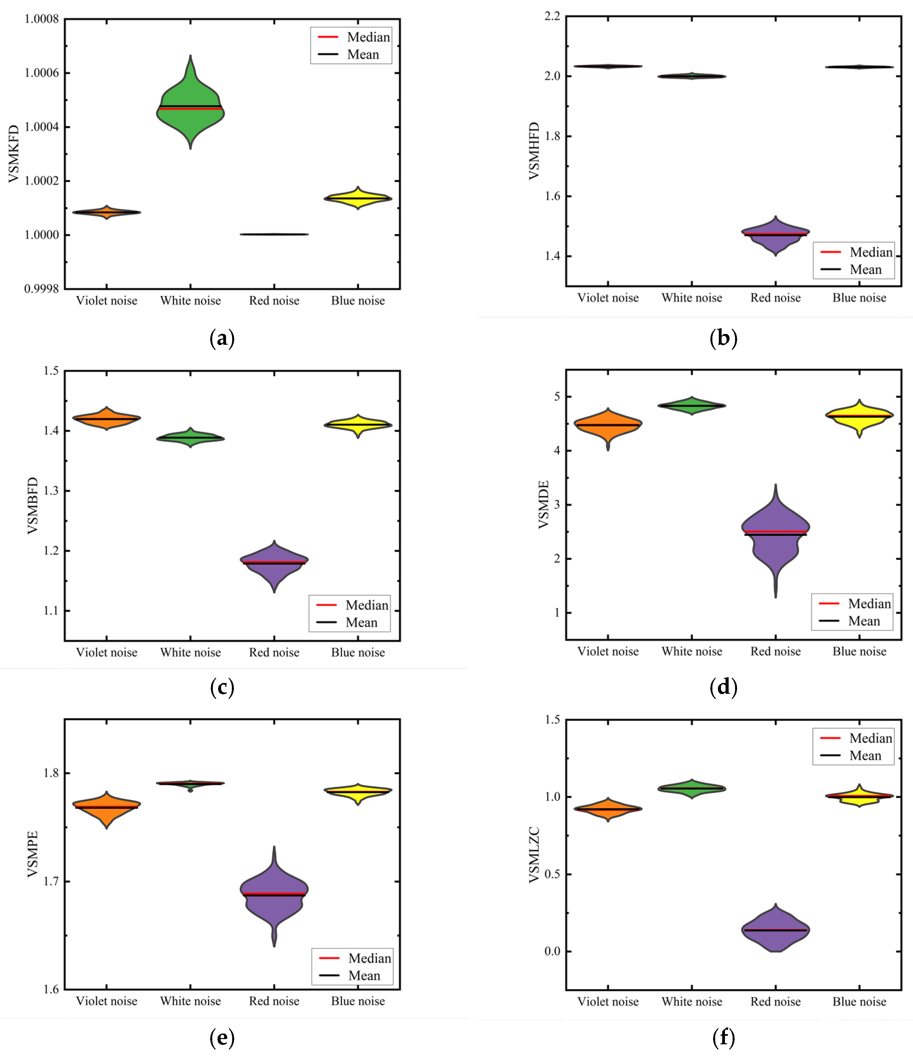
Figure 5 and Figure 6 depict the feature distribution of four noise signals for six metrics; we only provide the figures of and , as previously. As shown in Figure 5, all six nonlinear dynamic metrics are able to completely distinguish the red noise from the other three noise signals; among the feature distributions of the VSMKFD, there is no overlapping part for the feature distribution of four noise signals, which shows that all the noise signals can be better distinguished; for the other five metrics, the violet noise, white noise, and blue noise appear to overlap, with the overlap of VSMDE being the largest, making it difficult to differentiate between the three noise signals and with a large variance in the signal features.
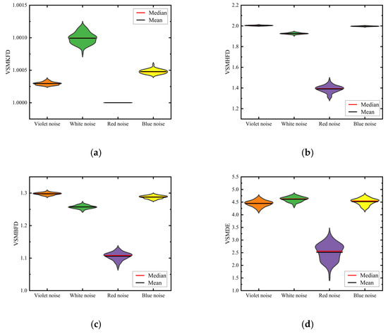
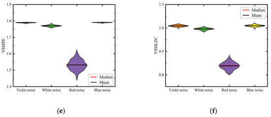
Figure 5.
The feature distribution of four noise signals for six metrics (): (a) VSMKFD; (b) VSMHFD; (c) VSMBFD; (d) VSMDE; (e) VSMPE; (f) VSMLZC.
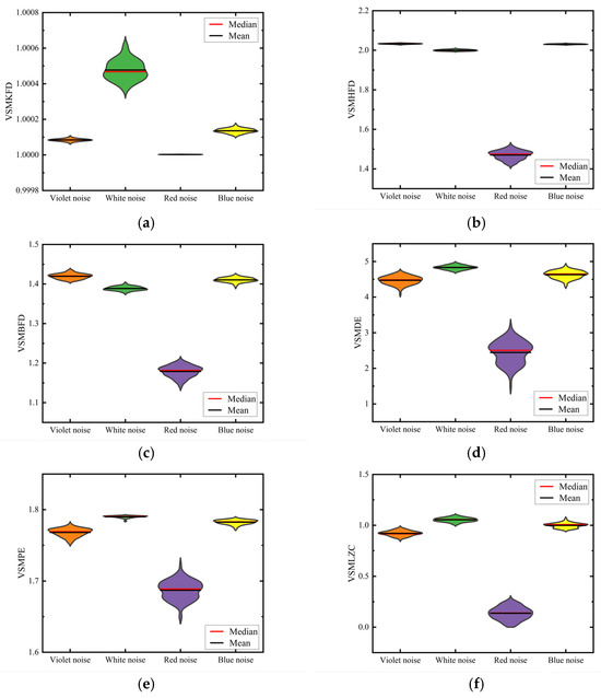
Figure 6.
The feature distribution of four noise signals for six metrics (): (a) VSMKFD; (b) VSMHFD; (c) VSMBFD; (d) VSMDE; (e) VSMPE; (f) VSMLZC.
From Figure 6, the situation with is similar to that with ; all six nonlinear dynamic metrics can distinctly differentiate red noise from the other three noise types; in the case of the VSMKFD, violet noise and blue noise overlap only slightly. Conversely, for the other five metrics, there is a noticeable overlap among the violet, white, and blue noise, with the most significant overlap continuing to be in the VSMDE. In summary, the VSMKFD demonstrates superior capability in differentiating noisy signals, further attesting to its efficacy.
3.3. The Chaotic Signal Classification Experiment
In addition to the noise signal classification experiment, we conducted further tests using three distinct chaotic signals to validate the feature extraction capabilities of the proposed VSMKFD. Figure 7 shows the waveforms of the Henon [33], Chen [34], and Rossler [35] signals in one sample.
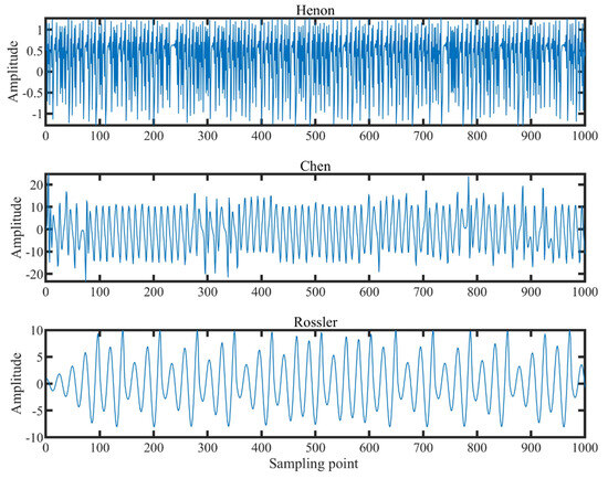
Figure 7.
The waveforms of three chaotic signals.
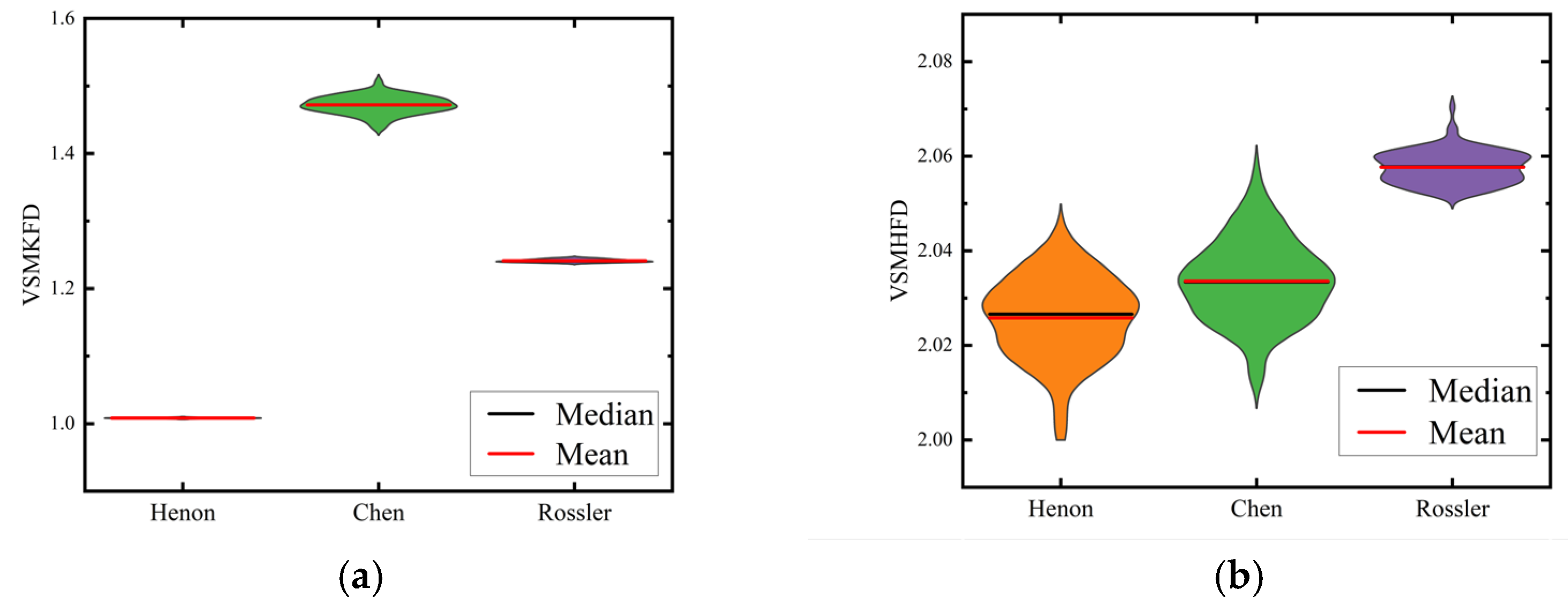
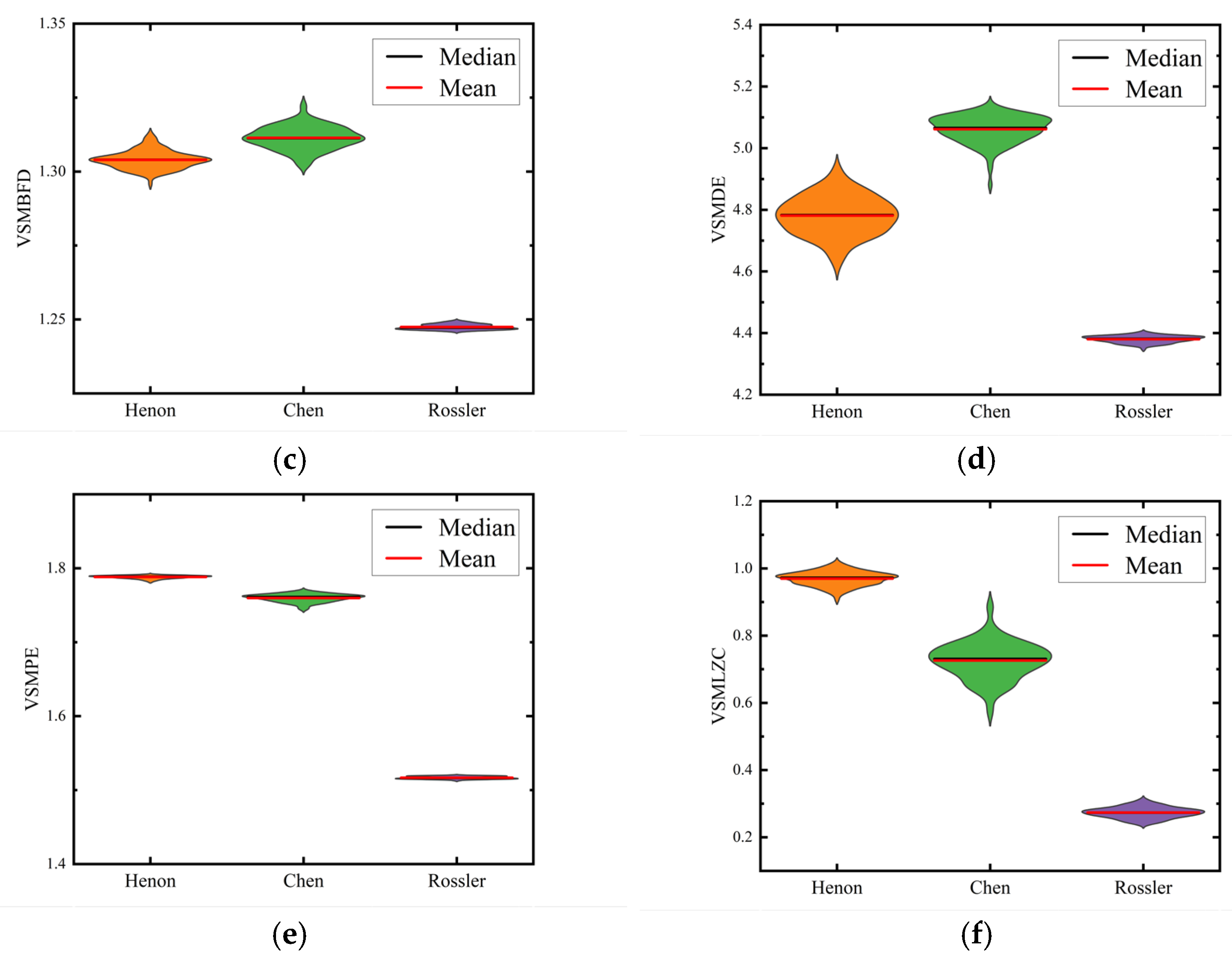
Figure 8 and Figure 9 show the feature distribution of six metrics for chaotic signals. As before, we present only the scenarios of and . It can be observed from Figure 8 and Figure 9, that whether or , there is no overlapping distribution area in the VSMKFD, and the means of three chaotic signals also differ greatly, which indicates that the three kinds of chaotic signals can be distinguished; all three chaotic signals produce a large area of overlap in the distribution map of the VSMHFD; neither the VSMBFD nor the VSMDE can fully distinguish between the three chaotic signals; both the VSMPE and the VSMLZC can only distinguish the Rossler signal, while the distributions of Henon and Chen signals have large overlaps. With the above analysis, we can see that the VSMKFD has better classification performance on chaotic signals.
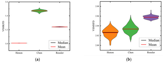
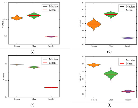
Figure 8.
The feature distribution of three chaotic signals for six metrics (): (a) VSMKFD; (b) VSMHFD; (c) VSMBFD; (d) VSMDE; (e) VSMPE; (f) VSMLZC.
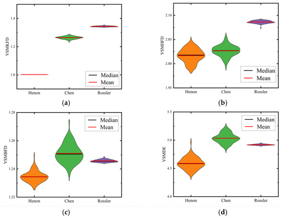
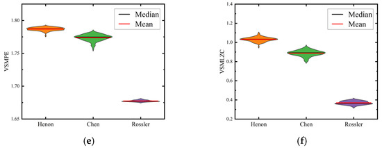
Figure 9.
The feature distribution of three chaotic signals for six metrics (): (a) VSMKFD; (b) VSMHFD; (c) VSMBFD; (d) VSMDE; (e) VSMPE; (f) VSMLZC.
4. The Feature Extraction Experiment on Ship-Radiated Noise
To underscore the superiority of the proposed VSMKFD in SRN analysis, this section undertook feature extraction experiments on SRNs of different categories and the same categories. It is imperative to note that the nonlinear dynamic metrics and corresponding parameter configurations employed for comparative analysis align precisely with those delineated in Section 3.
4.1. Case 1: Different Categories of Ship-Radiated Noise
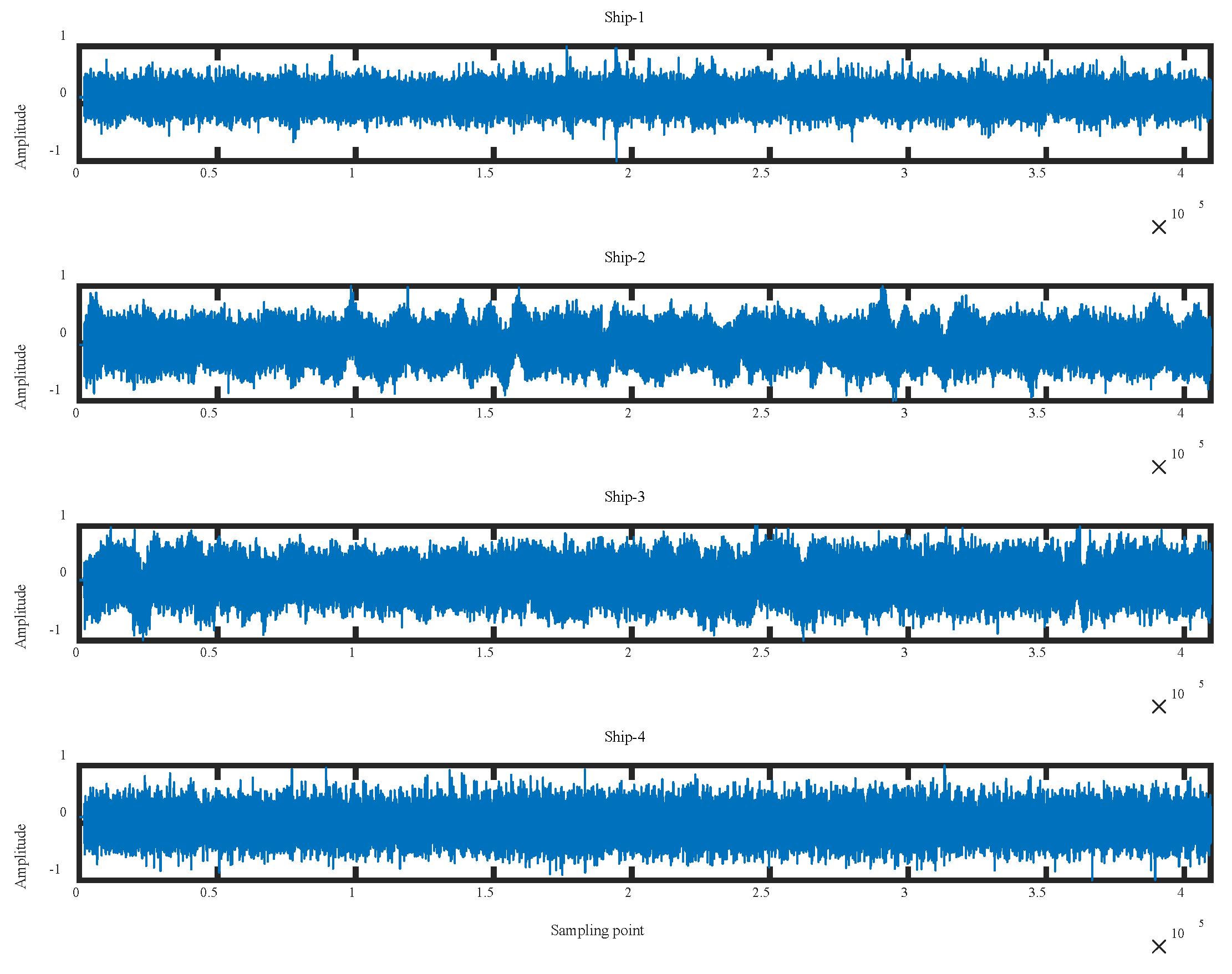
To evaluate the ability of the VSMKFD in feature extraction, the four different categories of SRN used in this experiment are from the National Park Service [36], including the categories of state ferry, freighter, outboard engine (60 hp) at 20 knots, and small diesel-engine-powered ships underwater recording, named Ship-1, Ship-2, Ship-3, and Ship-4. For each category of SRN, we adopted a sampling frequency of 44,100 Hz and selected 200 samples; each of these samples encompassed 2048 sampling points. Figure 10 displays the normalized waveform of four categories of SRN.
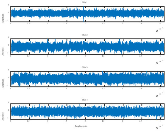
Figure 10.
The normalized waveform of four categories of SRN.
First, half of the samples of each class from the SRN were randomly selected as the training set, and the other half were selected as the test set. This resulted in 100 training samples and an equivalent number of test samples, which were trained using a K-n neighbor (KNN) classifier to conduct the classification experiment. Table 1 reveals the highest average recognition rate under different feature numbers. From Table 1, for the six nonlinear dynamic metrics, as the number of extracted features continues to increase, the recognition rate first improves, then stabilizes, and finally decreases slightly, and the overall recognition effect presents an upward trend. For the VSMKFD, no matter the number of features extracted, it has the highest classification accuracy of the other five metrics, with a 99.5% recognition rate in all cases except for single features and ten features; the recognition rate of the VSMHFD reaches its highest only at five features. From the above, compared to other nonlinear dynamic metrics, the VSMKFD exhibits enhanced SRN classification capability.

Table 1.
The highest average recognition rate under different feature numbers (%).
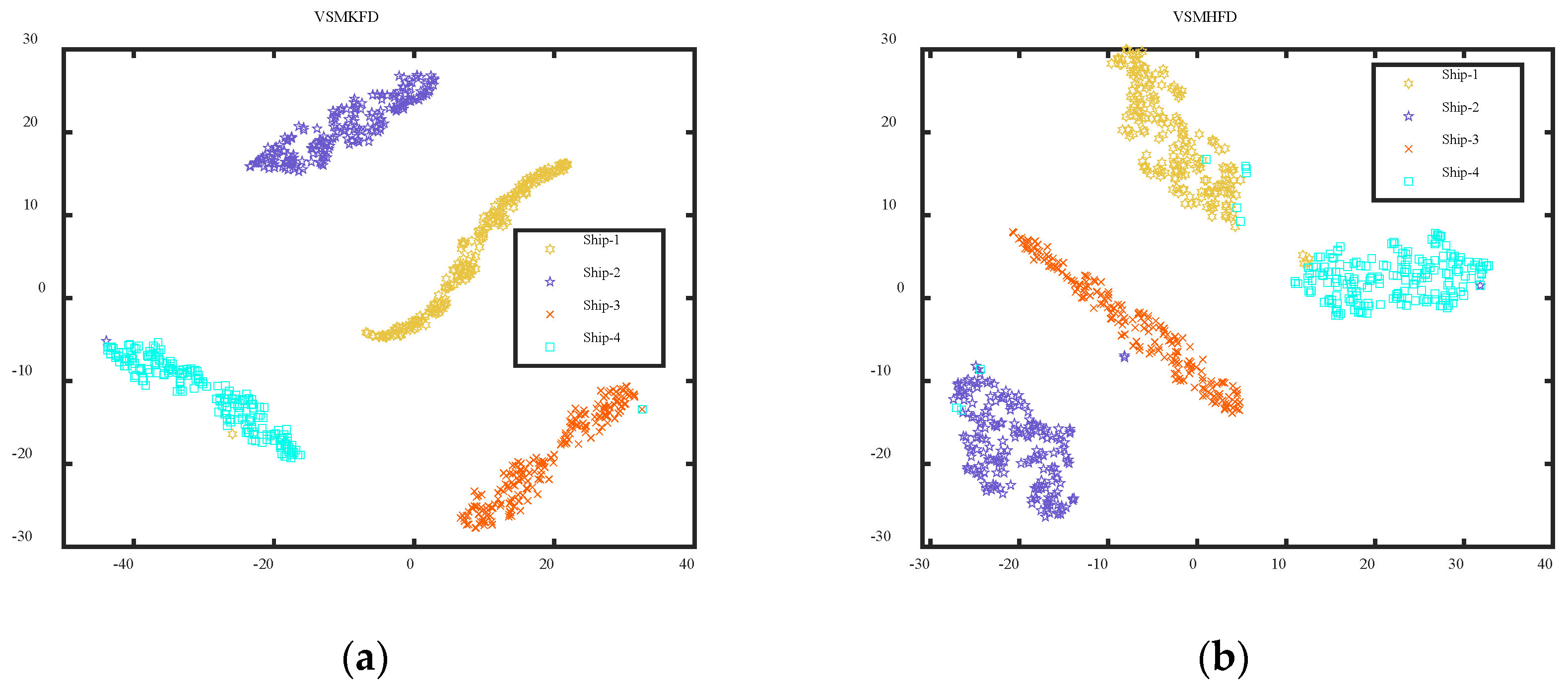
Then, to more intuitively demonstrate the advantages of the VSMKFD in distinguishing SRN, we calculate the different nonlinear dynamic metric values of each signal under 10 scales to obtain the corresponding 10-dimensional spatial feature set. Then the t-stochastic neighbor embedding (t-SNE) was visualized to map each 10-dimensional object onto a point in 2-dimensional phase space to visualize the extracted features. Figure 11 depicts the visualization results of extracted features of four ship signals. From Figure 11, it can be seen that the VSMKFD has the best visualization result; the features of the various kinds of SRN in the VSMKFD are relatively centralized and have nearly no overlapping sections. However, the features extracted from the other nonlinear dynamic metrics suffer from varying degrees of overlap and decentralization. For example, the features of each SRN in the VSMHFD are more decentralized than those of VSMKFD, especially in the distribution of Ship-1, Ship-2, and Ship-4. For the VSMBFD, VSMDE, VSMPE, and VSMLZC, Ship-1 and Ship-4 have wide overlapped areas. In addition, the distribution of Ship-3 in VSMLZC was more decentralized, being split into two parts. Therefore, the proposed VSMKFD can better recognize different categories of SRN compared to other nonlinear dynamic metrics.

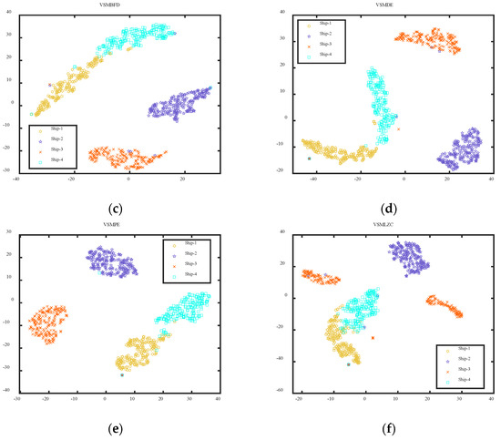
Figure 11.
The visualization results of extracted features of four ship signals: (a) VSMKFD; (b) VSMHFD; (c) VSMBFD; (d) VSMDE; (e) VSMPE; (f) VSMLZC.
4.2. Case 2: Same Categories of Ship-Radiated Noise
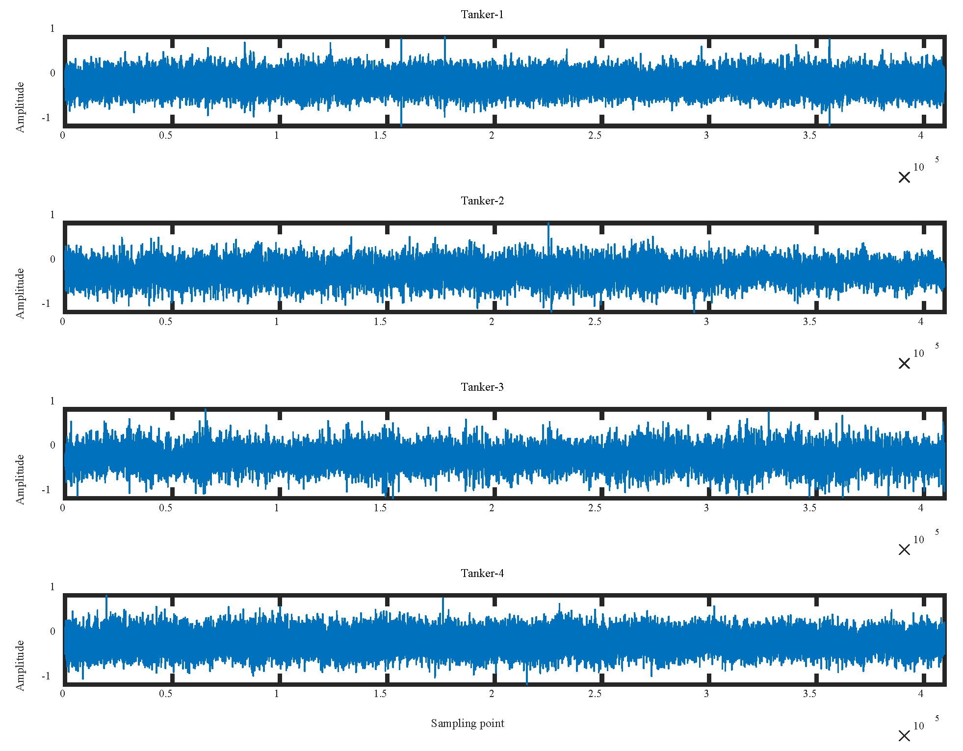
In this section, we select four tanker singles from the DeepShip database [37], including KIRKEHOLMEN, CARIBBEAN SPIRIT, CHERRY GALAXY, and CHAMPION EBONY, named as Tanker-1, Tanker-2, Tanker-3, and Tanker-4. In addition, the sampling frequency is 32,000 Hz, and we also selected 200 samples, each encompassing 2048 sampling points. Figure 12 displays the normalized waveform of four tanker signals.
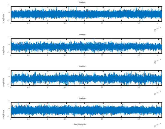
Figure 12.
The normalized waveform of four tanker signals.
To evaluate the practicality of the VSMKFD in feature extraction of SRN, the recognition rate was calculated using an approach that was similar to that of Case 1. Table 2 demonstrates the highest average recognition rate under different feature numbers. It can be observed in Table 2 that VSMKFD has the highest recognition rate under different numbers of features; the recognition rates are higher than 98% under multi features and even reach 99.25% under four features, while the recognition rates of the other five metrics are all below 96%, whereas the recognition rates of the VSMDE, VSMPE, and VSMLZC are all below 90%, and the recognition rate of the VSMLZC can only reach 80%. Based on the above analysis, the proposed VSMKFD still performed best on the feature extraction of the SRN.
Table 2.
The highest average recognition rate under different feature numbers (%).
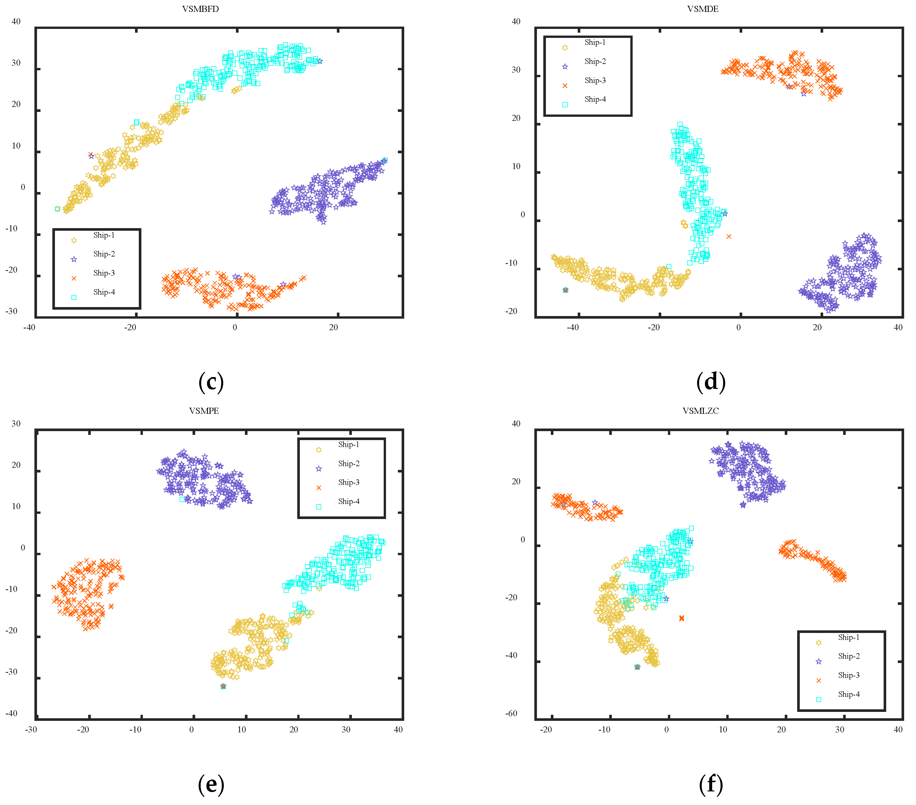
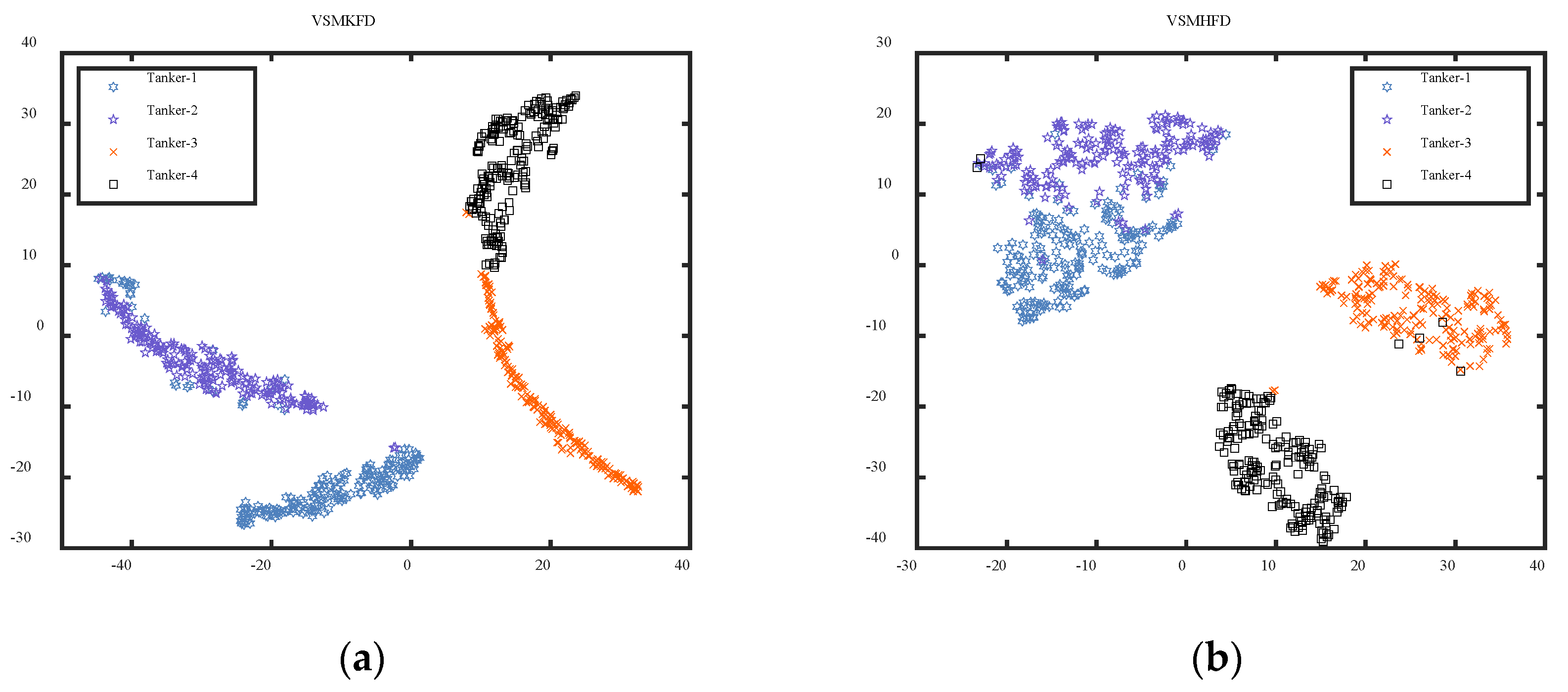
Aiming to further verify the efficiency of the proposed VSMKFD, we conducted a feature extraction experiment for four tanker signals, and the visualization results of the extracted features of four tanker signals are shown in Figure 13. From Figure 13, it is evident that the distribution of four signals in the VSMKFD can be nicely separated with scarcely any overlap of features. In contrast, the other five metrics all suffer from varying degrees of feature overlap. Neither the VSMHFD nor the VSMBFD can distinguish between Tanker-1 and Tanker-2 due to overlapping features; VSMDE cannot even distinguish between Tanker-3 and Tanker-4; the most serious are VSMPE and VSMLZC, where all four signals have overlapping features. The t-SNE experiment shows that the VSMKFD is more effective for the SRN recognition task than other nonlinear dynamic metrics.

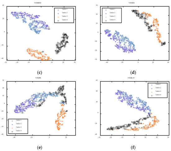
Figure 13.
The visualization results of extracted features of four tanker signals: (a) VSMKFD; (b) VSMHFD; (c) VSMBFD; (d) VSMDE; (e) VSMPE; (f) VSMLZC.
5. Conclusions
In this study, a novel nonlinear dynamic metric, termed VSMKFD, was proposed and applied to the feature extraction of SRN. The simulated and real signal experiments demonstrate the validity of the proposed method. The main conclusions are summarized as follows:
- (1)
- The VSMKFD was proposed by combining a variable-step multiscale process with KFD, which can improve the feature extraction performance of KFD and fully exploit signal information buried in multiscale.
- (2)
- It is validated that the VSMKFD is able to effectively reflect the frequency change of the chirp signal and has a stronger distinguishing capability for noise signals and chaotic signals than other nonlinear dynamic metrics.
- (3)
- The VSMKFD outperforms the VSMHFD, VSMBFD, VSMDE, VSMPE, and VSMLZC in classifying different and the same categories of SRN and achieves the highest recognition rate and more stable performance, which effectively improves the feature extraction performance.
Author Contributions
Y.L.: methodology, software, writing—original draft, writing—review and editing, and funding acquisition. Y.Z.: methodology, software, data curation, and writing—original draft. S.J.: writing—review and editing, visualization, and supervision. All authors have read and agreed to the published version of the manuscript.
Funding
This research was funded by the National Natural Science Foundation of China (grant no. 62371388), Xi’an University of Technology Excellent Seed Fund (grant no. 252082302), Qin Chuangyuan Innovation Platform (grant no. 23TSPT0002), and Scientists+Engineers Team (grant no. 23KGDW0011).
Data Availability Statement
The datasets analyzed during the current study are available from the corresponding author on reasonable request.
Conflicts of Interest
The authors declare no conflict of interest.
Nomenclature
| SRN | ship-radiated noise |
| LZC | Lempel–Ziv complexity |
| SE | sample entropy |
| FE | fuzzy entropy |
| PE | permutation entropy |
| DE | dispersion entropy |
| PLZC | permutation Lempel–Ziv complexity |
| DLZC | dispersion Lempel–Ziv complexity |
| NCDF | normal cumulative distribution function |
| DELZC | dispersion entropy-based Lempel–Ziv complexity |
| FDLZC | fluctuation-based dispersion Lempel–Ziv complexity |
| KFD | Katz fractal dimension |
| BFD | box fractal dimension |
| HFD | Higuchi fractal dimension |
| VSMKFD | variable-step multiscale Katz fractal dimension |
| VSMHFD | variable-step multiscale Higuchi fractal dimension |
| VSMBFD | variable-step multiscale box fractal dimension |
| VSMDE | variable-step multiscale dispersion entropy |
| VSMPE | variable-step multiscale permutation entropy |
| VSMLZC | variable-step multiscale Lempel–Ziv complexity |
References
- Li, G.; Hou, Y.; Yang, H. A novel method for frequency feature extraction of ship radiated noise based on variational mode decomposition, double coupled Duffing chaotic oscillator and multivariate multiscale dispersion entropy. Alex. Eng. J. 2022, 61, 6329–6347. [Google Scholar] [CrossRef]
- Gassmann, M.; Wiggins, S.M.; Hildebrand, J.A. Deep-water measurements of container ship radiated noise signatures and directionality. J. Acoust. Soc. Am. 2017, 142, 1563–1574. [Google Scholar] [CrossRef] [PubMed]
- Wang, S.; Zeng, X. Robust underwater noise targets classification using auditory inspired time-frequency analysis. Appl. Acoust. 2014, 7, 68–76. [Google Scholar] [CrossRef]
- Yuan, F.; Ke, X.; Cheng, E. Joint Representation and Recognition for Ship-Radiated Noise Based on Multimodal Deep Learning. J. Mar. Sci. Eng. 2019, 7, 380. [Google Scholar] [CrossRef]
- Ke, X.; Yuan, F.; Cheng, E. Integrated optimization of underwater acoustic ship-radiated noise recognition based on two-dimensional feature fusion. Appl. Acoust. 2020, 159, 107057. [Google Scholar] [CrossRef]
- Li, Y.; Geng, B.; Tang, B. Simplified coded dispersion entropy: A nonlinear metric for signal analysis. Nonlinear Dyn. 2023, 111, 9327–9344. [Google Scholar] [CrossRef]
- Li, Y.; Zhang, C.; Zhou, Y. A Novel Denoising Method for Ship-Radiated Noise. J. Mar. Sci. Eng. 2023, 11, 1730. [Google Scholar]
- Li, Y.; Tang, B.; Jiao, S.; Su, Q. Snake Optimization-Based Variable-Step Multiscale Single Threshold Slope Entropy for Complexity Analysis of Signals. IEEE Trans. Instrum. Meas. 2023, 72, 6505313. [Google Scholar] [CrossRef]
- Siddagangaiah, S.; Li, Y.; Guo, X.; Chen, X.; Zhang, Q.; Yang, K.; Yang, Y. A complexity-based approach for the detection of weak signals in ocean ambient noise. Entropy 2016, 18, 101. [Google Scholar] [CrossRef]
- Hu, Q.; Li, Y.; Sun, X.; Chen, M.; Bu, Q.; Gong, B. Integrating test device and method for creep failure and ultrasonic response of methane hydrate-bearing sediments. Rev. Sci. Instrum. 2023, 94, 025105. [Google Scholar] [CrossRef]
- Lempel, A.; Ziv, J. On the complexity of finite sequences. IEEE Trans. Inf. Theory 1976, 22, 75–81. [Google Scholar] [CrossRef]
- Xue, Q.; Xu, B.; He, C.; Liu, F.; Ju, B.; Lu, S.; Liu, Y. Feature Extraction Using Hierarchical Dispersion Entropy for Rolling Bearing Fault Diagnosis. IEEE Trans. Instrum. Meas. 2021, 70, 1–11. [Google Scholar] [CrossRef]
- Richman, J.S.; Randall, M.J. Physiological time-series analysis using approximate entropy and sample entropy. Am. J. Physiol. Heart Circ. Physiol. 2000, 278, H2039–H2049. [Google Scholar] [CrossRef] [PubMed]
- Chen, W.; Wang, Z.; Xie, H.; Yu, W. Characterization of Surface EMG Signal Based on Fuzzy Entropy. IEEE Trans. Neural Syst. Rehabil. Eng. 2007, 15, 266–272. [Google Scholar] [CrossRef] [PubMed]
- Bandt, C.; Pompe, B. Permutation entropy: A natural complexity measure for time series. Phys. Rev. Lett. 2002, 88, 174102. [Google Scholar] [CrossRef] [PubMed]
- Rostaghi, M.; Azami, H. Dispersion Entropy: A Measure for Time-Series Analysis. IEEE Signal Process. Lett. 2016, 23, 610–614. [Google Scholar] [CrossRef]
- Simons, S.; Abásolo, D. Distance-Based Lempel-Ziv Complexity for the Analysis of Electroencephalograms in Patients with Alzheimer’s Disease. Entropy 2017, 19, 129. [Google Scholar] [CrossRef]
- Bai, Y.; Liang, Z.; Li, X. A Permutation Lempel-Ziv complexity measure for EEG analysis. Biomed. Signal Process. Control 2015, 19, 102–114. [Google Scholar] [CrossRef]
- Mao, X.; Shang, P.; Xu, M.; Peng, C. Measuring time series based on multiscale dispersion Lempel-Ziv complexity and dispersion entropy plane. Chaos Solitons Fractals 2020, 137, 109868. [Google Scholar] [CrossRef]
- Li, Y.; Geng, B.; Jiao, S. Dispersion entropy-based Lempel-Ziv complexity: A new metric for signal analysis. Chaos Solitons Fractals 2022, 161, 112400. [Google Scholar] [CrossRef]
- Li, Y.; Jiao, S.; Geng, B. Refined composite multiscale fluctuation-based dispersion Lempel-Ziv complexity for signal analysis. ISA Trans. 2023, 133, 273–284. [Google Scholar] [CrossRef] [PubMed]
- Mendelbrot, B. How long is the coast of Britain? Statistical self-similarity and fractional dimension. Science 1967, 156, 636–638. [Google Scholar] [CrossRef] [PubMed]
- Katz, M.J. Fractals and the analysis of waveforms. Comput. Biol. Med. 1988, 18, 145–156. [Google Scholar] [CrossRef] [PubMed]
- Gagnepain, J.J.; Roques-Carmes, C.F. Fractal approach to two-dimensional and three-dimensional surface roughness. Wear 1986, 109, 119–126. [Google Scholar] [CrossRef]
- Higuchi, T. Approach to an irregular time series on the basis of the fractal theory. Phys. D Nonlinear Phenom. 1988, 37, 277–283. [Google Scholar] [CrossRef]
- Hu, J.; Tung, W.; Gao, J. Detection of low observable targets within sea clutter by structure function based multifractal analysis. IEEE Trans. Antenn. Propag. 2006, 54, 136–143. [Google Scholar] [CrossRef]
- Burlaga, L.; Klein, L. Fractal structure of the inter planetary magnetic field. J. Geophys. Res. Space Phys. 1986, 91, 347–350. [Google Scholar] [CrossRef]
- Shi, C.-T. Signal Pattern Recognition Based on Fractal Features and Machine Learning. Appl. Sci. 2018, 8, 1327. [Google Scholar] [CrossRef]
- Humeau-Heurtier, A. Multiscale Entropy Approaches and Their Applications. Entropy 2020, 22, 644. [Google Scholar] [CrossRef]
- Wu, S.-D.; Wu, C.-W.; Lin, S.-G.; Lee, K.-Y.; Peng, C.-K. Analysis of complex time series using refined composite multiscale entropy. Phys. Lett. A 2014, 378, 1369–1374. [Google Scholar] [CrossRef]
- Li, Y.; Liang, L.; Zhang, S. Hierarchical Refined Composite Multi-Scale Fractal Dimension and Its Application in Feature Extraction of Ship-Radiated Noise. Remote Sens. 2023, 15, 3406. [Google Scholar] [CrossRef]
- Su, Z.; Shi, J.; Luo, Y.; Shen, C.; Zhu, Z. Fault severity assessment for rotating machinery via improved Lempel-Ziv complexity based on variable-step multiscale analysis and equiprobable space partitioning. Meas. Sci. Technol. 2022, 33, 055018. [Google Scholar] [CrossRef]
- Hénon, M. A two-dimensional mapping with a strange attractor. Commun. Math. Phys. 1976, 50, 69–77. [Google Scholar] [CrossRef]
- Chen, C.-T. Signals and Systems; Oxford University Press: New York, NY, USA, 2004; p. 453. [Google Scholar]
- Rössler, O.E. An equation for continuous chaos. Phys. Lett. A 1976, 57, 397–398. [Google Scholar] [CrossRef]
- National Park Service. Available online: https://www.nps.gov/index.htm (accessed on 28 July 2023).
- Muhammad, I.; Zheng, J.; Shahid, A.; Muhammad, I.; Zafar, M.; Umar, H. DeepShip: An underwater acoustic benchmark dataset and a separable convolution based autoencoder for classification. Expert. Syst. Appl. 2021, 183, 115270. [Google Scholar]


Disclaimer/Publisher’s Note: The statements, opinions and data contained in all publications are solely those of the individual author(s) and contributor(s) and not of MDPI and/or the editor(s). MDPI and/or the editor(s) disclaim responsibility for any injury to people or property resulting from any ideas, methods, instructions or products referred to in the content. |
© 2023 by the authors. Licensee MDPI, Basel, Switzerland. This article is an open access article distributed under the terms and conditions of the Creative Commons Attribution (CC BY) license (https://creativecommons.org/licenses/by/4.0/).