Article

Enhanced Impedance Control of Cable-Driven Unmanned Aerial Manipulators Using Fractional-Order Nonsingular Terminal Sliding Mode Control with Disturbance Observer Integration

1
College of Mechanical Engineering, Jiangsu University of Technology, Changzhou 213001, China
2
College of Mechanical and Electrical Engineering, Nanjing University of Aeronautics and Astronautics, Nanjing 210016, China
*
Author to whom correspondence should be addressed.
Fractal Fract. 2024, 8(10), 579; https://doi.org/10.3390/fractalfract8100579
Submission received: 18 August 2024 / Revised: 26 September 2024 / Accepted: 28 September 2024 / Published: 30 September 2024

Abstract

:
The article presents a novel control strategy for cable-driven aerial manipulators (UAMs) aimed at enhancing impedance control during contact operations in complex environments. A fractional-order nonsingular terminal sliding mode control (FONTSMC) integrated with a disturbance observer (DOB) is proposed to improve the robustness and precision of the UAM under lumped disturbances. This developed approach utilizes the flexibility of fractional calculus, the finite-time stability of nonsingular terminal sliding mode, and the real-time disturbance estimation capabilities of the DOB to ensure smooth and compliant contact interactions. The effectiveness of the proposed control strategy is validated through comprehensive simulation studies, which demonstrate significant improvements in control performance, stability, and disturbance rejection when compared to traditional methods. The results indicate that the FONTSMC-DOB framework is highly suitable for complex aerial manipulation tasks, offering both theoretical and practical insights into the design of advanced control systems for UAMs.

1. Introduction

At present, unmanned aerial vehicles (UAVs), with their autonomy and capability for remote control, make it possible to accomplish a diverse array of challenging tasks. Installing a manipulator on the UAV, also known as an unmanned aerial manipulator (UAM), allows it to conduct manipulation tasks, which we refer to as aerial manipulation [1].The tasks a UAM can undertake aerial grasping [2], industrial inspection [3], turning valves [4], water sampling [5], canopy sampling [6], among others. UAM operation control involves the knowledge and technology of many subject areas such as system modeling, motion planning, and UAM control theory, which is a challenging and practical research direction in the field of robotics Engineering. In general, developing a reliable and effective controller for UAMs is difficult due to the complex and interconnected dynamics involved, where the motion of the manipulator affects the motion of the UAV [7,8]. The operation mode of a UAM consists of two categories based on its relative position to the object to be operated [9]. One is non-contact operation, which only requires controlling the precise movement of the robotic arm. An alternative method is contact operation, necessitating the regulation of the force applied between the end-effector and the object being manipulated, alongside managing the movement of the robotic arm. This paper emphasizes the exploration of control strategies applicable to contact operations in UAM.
In order to achieve stable aerial contact control, researchers have explored various disturbance rejection strategies for implementing the UAMs. These strategies include active disturbance rejection control [10], linear active disturbance rejection control [11], neural network control [12], sliding mode control based on disturbance observer [13], and so on. Studies indicate that UAMs commonly utilize compliance control to enhance operational stability. Common methods of compliance control include conductivity control methods and impedance control methods [14]. Among them, impedance control is a control strategy used to regulate the relationship between force and displacement of the end-effector of a robotic arm when it comes into contact with the environment. It enables a manipulator to produce a corresponding change in displacement when it encounters an external force by equating the relationship between force (or moment) and displacement (or angle) to a mechanical impedance model (e.g., a spring-mass-damping system). Impedance control strategies are widely used for flexible operation or cooperative work of the aerial manipulators. For example, Xu et al. presented an image-based impedance control strategy for force tracking in UAMs, integrating visual servoing with adaptive impedance control to achieve stable, effective force tracking without position measurement, validated through experimental results in a board cleaning task [15]. Byun et al. proposed an image-based, time-varying force tracking controller for UAMs, leveraging visual features and RISATE-based impedance filtering to ensure stable, accurate force interaction with static surfaces, validated through experiments demonstrating improved force-tracking performance [16]. In fact, several control strategies have been proposed to achieve stable and effective impedance control in the presence of nonlinear characteristics. Bonilla et al. proposed an adaptive control method for 2-degree-of-freedom (DOF) robotic manipulator impedance control, enabling dynamic parameter adjustment, which ensured stable, precise interactions and effective handling of uncertainties across various scenarios [17]. Jin et al. introduced a model predictive control approach for impedance control in multi-contact industrial manipulation, ensuring robust and stable interactions across multiple surfaces while achieving desired force levels [18]. Fuzzy logic control was employed by Kong et al. for impedance regulation in a robotic arm, with parameters adjusted based on qualitative descriptions, enabling smooth transitions and robust, stable operation [19]. Ruggiero et al. introduced a sliding mode control (SMC) strategy for impedance regulation in uncertainty robotic manipulator, effectively handling nonlinear dynamics and disturbances, resulting in improved stability and precision in force tracking [20].
Among the above control strategies, SMC is a widely utilized control strategy known for its robustness in handling the lumped disturbances, but in practice it is subject to high-frequency oscillations that can degrade performance and cause motor damage [21,22]. To overcome SMC limitations, terminal sliding mode (TSM) [23], an enhanced variant of conventional SM known for achieving finite-time stability, was introduced. Following its inception, various evolved versions including fast TSM (FTSM) [24], nonsingular TSM (NTSM) [25], and continuous NTSM [23] were developed and subjected to further research, expanding the applicability and effectiveness of SMC techniques. Recent efforts have focused on designing disturbance observer (DOB)-based NTSM controllers [26,27], combining the strengths of both DOB and NTSM. These controllers not only overcome the performance limitations of each approach but also effectively suppress the system’s lumped disturbances, enhancing overall control performance. However, most existing DOB-based NTSM controllers are limited to integer-order (IO) controllers, using only IO integrators and differentiators [28]. It is widely recognized that fractional order (FO) SMC incorporates fractional calculus, offering greater design flexibility and improved performance in systems with complex, time-varying dynamics [29,30,31]. Recently, control schemes based on DOB and fractional order nonsingular terminal sliding mode (FONTSM-DOB) have been proposed and studied for robotic manipulators [32,33,34]. Although these studies have made notable advancements, additional enhancements are still possible. The main contributions of this paper are summarized in the following three points:
  • A FONTSM-DOB control strategy is developed to achieve impedance control for UAMs during contact operations with the external environment under lumped disturbances. This strategy integrates the strengths of fractional-order (FO) calculus, nonsingular terminal sliding mode (NTSM), and disturbance observer (DOB) techniques, significantly enhancing UAM control performance while ensuring smooth and compliant contact interactions. This approach effectively addresses the challenges of operating in uncertain environments, providing both robustness and precision in aerial manipulation tasks.
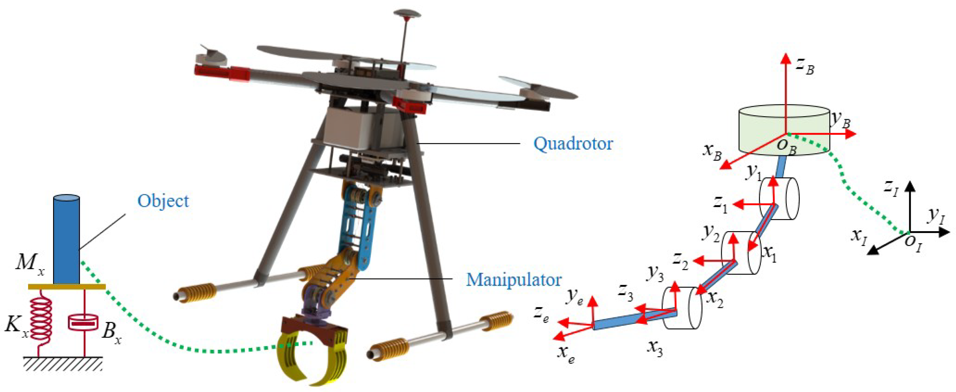
  • Given the redundancy of the designed UAM, the inverse kinematics problem is addressed using the Jacobian matrix. Additionally, the flexibility of the links and cables is modeled as joint flexibility, allowing for the establishment of a rigid-flexible coupling dynamic model. This approach more accurately captures the dynamic characteristics of the aerial manipulator, providing a realistic representation of its behavior during operation.
  • The UAM designed in this paper incorporates a cable-driven mechanism, where the drive units (e.g., motors, reducers) are mounted at the manipulator’s base. This design remotely transmits force and torque to the robotic arm’s joints via flexible cables, significantly reducing the manipulator’s inertia and achieving a lightweight overall structure. This approach not only enhances the manipulator’s dynamic performance but also optimizes the system’s structural efficiency, making it more suitable for complex aerial manipulation tasks.
The remainder of this paper is organized as follows: Section 2 details the kinematics and dynamics model of the cable-driven aerial manipulator. Section 3 presents the design of the DOB-based FONTSM controller and its stability analysis using Lyapunov theory. Two comparative simulation cases demonstrating the effectiveness of the proposed method are discussed in Section 4. Finally, Section 5 concludes the paper.

2. UAM Mathematical Model

When a UAM operates in contact with its surroundings, such as fruit picking, plant pruning, and power tower spanning, the operational target can be equated to a spring-mass-damping system [35]. A general dynamic model is presented for a UAM developed in this paper comprising of an unmanned quadrotor and a 3-link robotic arm, as shown in Figure 1. The joints of the manipulator utilize the cable-driven mechanism, while the end-effector is servo-driven. To comprehensively understand the interaction between the aerial manipulator and its environment, it is essential to consider the system’s behavior within a position control framework, particularly when contact forces are present. This behavior is best described in the operational space, necessitating the modeling of the aerial manipulator’s dynamics specifically within this space. This approach ensures a precise analysis of how the system responds to external forces during operation.
Remark 1
([36,37]). This study focuses on the fractional-order impedance control of a manipulator, with the quadrotor serving as a floating platform. For the purposes of this investigation, the dynamic behavior and control of the quadrotor are disregarded, allowing us to concentrate exclusively on the control strategies and performance of the manipulator.
Let us define that E I = x I , y I , z I represents the inertial frame, E B = x B , y B , z B represents the fuselage frame of the quadrotor, and ζ i = x i , y i , z i represents the manipulator frame, where i = 1 , 2 , 3 , e . The vector of the joint position is defined as q = q 1 , q 2 , q 3 T , and the Euler angles of the UAV in the inertial frame by η = [ ϕ , θ , ψ ] T . The transformation from the body frame to inertial frame can be described by a rotation matrix R B I [38]:
R B I = cos θ cos ψ sin φ sin θ cos ψ cos φ sin ψ cos φ sin θ cos ψ + sin φ sin ψ cos θ sin ψ sin φ sin θ sin ψ + cos φ cos ψ cos φ sin θ sin ψ sin φ cos ψ sin θ sin φ cos θ cos φ cos θ

2.1. Manipulator Kinematics

The forward kinematic equations of the manipulator can be obtained using the DH(Denavit–Hartenberg) parametric method [39]. Table 1 gives the cable-driven manipulator’s DH parameters, specifically link length a i , link twist α i , joint offset d i , and joint angle q i ( i = 1 , 2 , 3 ) .
The change in pose from neighboring joints ζ i 1 to ζ i can be described by the equivalent homogeneous transformation matrix T i   i 1 :
T i   i 1 = cos q i sin q i cos α i sin q i sin α i a i cos q i sin q i cos q i cos α i cos q i sin α i a i sin q i 0 sin α i cos α i d i 0 0 0 1
According to the forward kinematics formula of the manipulator, the pose of the end-effector frame with respect to the fuselage frame can be governed by:
T e B = T 3 1 1 B T q i T e 3
For the UAM presented in this paper, the Jacobian pseudo-inverse method will be used to solve the inverse kinematic equations. The Jacobian matrix is a mathematical tool that describes the mapping relationship between workspace velocities and joint-space velocities [40]. The mapping relationship between joint velocity and end-effector velocity is governed by:
v e = p ˙ e ω ˙ e = J ( q ) q ˙
where p ˙ e and ω ˙ e are the end-effector linear and angular velocities, respectively.
Since the proposed UAM is redundant and its Jacobian matrix is not a square matrix, it cannot be directly solved by Equation (4) for q ˙ . Set the end-effector’s pose as f ( q ) = p e , ω e T , the target joint angles as q d , the initial joint angles as q 0 , one gets:
f q d f q 0 + J q 0 q d q 0
The error of the joint angles is calculated as:
e q = f q d f q 0 J q 0 Δ q
The presence of redundancy leads to the existence of multiple solutions for the inverse kinematics of the manipulator whereas in this paper, the optimal solution is obtained by numerical iterative method, which minimizes the joint angle error. At the same time, the reduction of redundant rotation of joint angles is also considered, so the objective function is constructed so that its value is minimized. The expression of g ( Δ q , λ ) is as follows:
g ( Δ q , λ ) = Δ q T Δ q + λ T ( J Δ q e q )
where λ is the multiplicative factor.
The generalized solution of Δ q is given as:
Δ q = J e q + I n J J P
where I n is the unit matrix, P is the arbitrary vector, J = J T J J T 1 is the right pseudo-inverse of J .
Therefore, the kinematic inverse solution of the manipulator can be obtained by associating Equations (4)–(8) as:
q d = Δ q + q 0

2.2. Manipulator Dynamics

Theorem 1.
The Newton–Euler method is a fundamental approach to robot dynamics that combines Newton’s second law of linear motion and Euler’s equations of rotation to describe the forces and moments acting on a robotic system. By systematically analyzing each link of the robot manipulator, the method provides a recursive framework for computing translational and rotational dynamics. A system dynamics model of the robot is obtained by considering the interactions between the connecting links, external forces, and joint actuation.
The dynamics model of the cable-driven aerial manipulator can be derived from the Newton–Euler equation as [41]:
M ( q ) q ¨ + C ( q , q ˙ ) q ˙ + G ( q ) = τ J T ( q ) F ext
where M ( q ) denotes the inertia matrix, C ( q , q ˙ ) denotes the Coriolis and centrifugal force terms, G ( q ) denotes the gravitational term, τ denotes the input torques, F ext denotes the unknown environmental constraints imposed on the end of the manipulator.
Remark 2.
The joint flexibility is modeled as a linear torsional spring system, where the force and moment at the joint are linearly correlated with variations in joint flexibility. Additionally, the motor rotors are approximated as uniform cylinders, simplifying the dynamic modeling of the system.
As outlined in Remark 2, the rigid-flexible coupled dynamics model of the UAM, which accounts for joint flexibility [42,43], can be formulated as follows:
J m δ ¨ + D m δ ˙ + M ( q ) q ¨ + C ( q , q ˙ ) q ˙ + G ( q ) = τ J T ( q ) F ext
where J m and D m are the motor inertia matrix and damping matrix, respectively. δ are the motor rotation angles.
The second-order impedance relation equation established by the difference between the contact force received at the end of the manipulator and the position deviation from the target trajectory is known as the desired impedance equation [44], which has the following expression:
M x X d X ¨ + B x X ˙ d X ˙ + K x X d X = J T ( q ) F ext = F e
where M x , B x , and K x represent the inertia, damping and stiffness coefficients of the impedance model, respectively. X , X ˙ , and X ¨ represent the displacement, velocity, and acceleration of the end-effector, respectively. X d , X ˙ d , and X ¨ d represent the desired displacement, velocity, and acceleration of the end-effector, respectively.
Remark 3.
Since impedance control is implemented in Cartesian space, it needs to be converted from joint space to Cartesian space for the above dynamics equations.
According to Remark 3 and Equation (4), the dynamics equation expressed in Cartesian space is given by:
M ( X ) X ¨ + C ( X , X ˙ ) X ˙ + G ( X ) = u F e
where M ( X ) = J T M ( q ) J 1 , C ( X , X ˙ ) = J T C ( q , q ˙ ) M ( q ) J 1 J ˙ J 1 , G ( X ) = J T G ( q ) , u = J T τ , X = x e x , x e z T , and X ˙ = x ˙ e x , x ˙ e z T .
Rewrite Equation (13) in the following form:
u = M ( X ) X ¨ + C ( X , X ˙ ) X ˙ + G ( X ) + F e + τ d = M ( X ) X ¨ + Φ
where Φ = C ( X , X ˙ ) X ˙ + G ( X ) + F e + τ d represents the lumped disturbances the incorporates the unmodeled characteristics and external perturbations.
Remark 4
([45]). In real-world scenarios, the motor performance constraints limit the impedance control of UAMs, leading to the phenomena of input saturation. However, the constrained yet appropriate control energy significantly affects the control performance and must not be disregarded by the controller.
Set δ ( u ) denotes the control input affected by the saturation nonlinearity, which can be denoted as [46]:
δ ( u ) = tanh u i = u i , max , u i u i , max u i , u i , min u i u i , max u i , min , u i u i , min
where u i , max and u i , min are the maximum and minimum values of the input torque, respectively. t a n h ( · ) represents the hyperbolic tangent function that provides smooth curves.

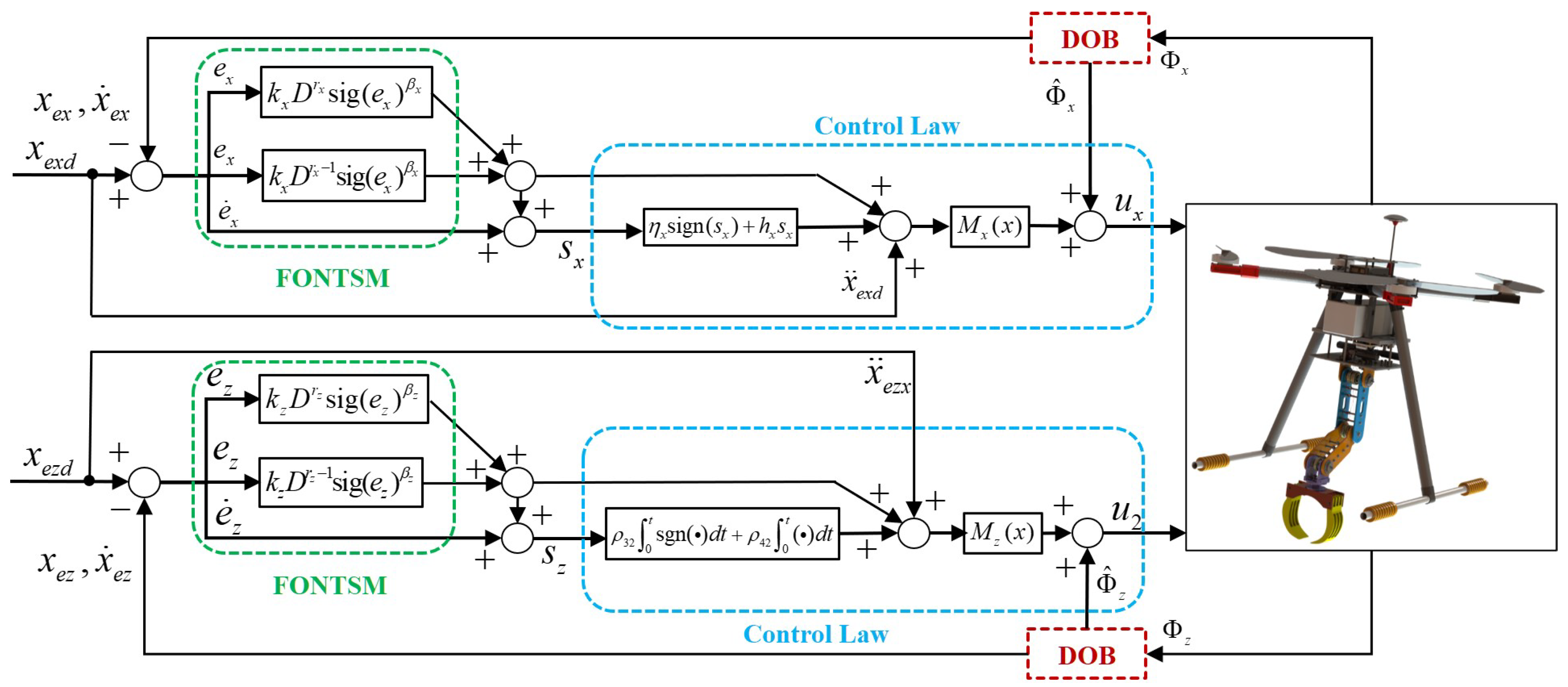
3. Controller Design

According to the modeling analysis presented in Section 2, it is evident that the motion range of the end effector of the designed cable-driven UAM is confined to the o x z plane, assuming the quadrotor’s motion is disregarded. This section uses the x-axis as an example to derive the design principle of the controller.

3.1. Disturbance Observer Design

In general, the lumped disturbances can be estimated using several methods, such as neural networks [47], fuzzy logic systems [48], and disturbance observers [49]. Disturbance Observers offer superior accuracy and robustness in real-time disturbance estimation compared to the other two methods. In this article, a fundamental nonlinear disturbance observer is proposed to estimate the unknown lumped disturbances Φ . Set x e x = x 1 , x ˙ e x = x 2 , the dynamics model in x-channel can be rewritten as:
x ˙ 1 = x 2 x ˙ 2 = M x 1 ( x ) δ u x Φ x
The design of the nonlinear disturbance observer is formulated as follows [50]:
Φ ^ ˙ x = l x x ˙ 2 M x 1 ( x ) δ u x Φ ^ x
where Φ ^ ˙ x denotes the disturbance estimation vector, and l x represents the observer gain.
The lumped disturbance estimation error is calculated as follows:
e Φ x = Φ ^ x Φ x
Combining Equation (18) with Equations (16) and (17), the dynamics of disturbance estimation error are derived and can be expressed as follows:
e ˙ Φ x = Φ ^ ˙ x Φ ˙ x = l x e Φ x
This indicates that the error in estimating disturbances will approach zero over time, given that the observer gain l x is selected to ensure that the system (19) is asymptotically stable. Additionally, it is important to mention that implementing the disturbance observer described in (17) necessitates the derivative of the state, which might require an extra sensor for its measurement in practice.

3.2. FONTSMC Design

Fractional calculus is an advanced mathematical concept that extends the traditional notions of integrals and derivatives to allow for real number orders. This means that instead of being limited to integer values, the operators of integration and differentiation can take on fractional values, creating a more nuanced framework for analysis and application. In the context of this study, the Caputo fractional derivative and integration techniques are specifically employed in the design of the controller [51]. This approach aims to enhance the design process by leveraging the properties of fractional derivatives and integrals, potentially offering improved performance and adaptability in the control system being examined.
Remark 5
([52,53]). Fractional order derivatives are commonly defined through fractional calculus, with the Riemann–Liouville and Caputo derivatives being the most frequently used. Unlike the Riemann–Liouville derivative, the Caputo fractional derivative allows initial conditions to be expressed in integer orders, simplifying the handling of known physical system conditions such as initial position, velocity, or acceleration. Additionally, the Riemann-Liouville derivative’s performance is more sensitive to initial conditions, complicating controller parameterization. Consequently, the Caputo derivative is often preferred for systems requiring robust and adaptive control in practical applications.
Theorem 2.
The definition of γ-th order Caputo fractional derivative and integration can be given as follows:
t 0 D t γ f ( t ) = 1 Γ ( m a ) t 0 t f ( m ) ( τ ) ( t τ ) α m + 1 d τ , t > t 0
where m 1 < γ < m , m N , and Γ ( · ) represents the Gamma function. In this article, the formula t 0 D t γ is replaced by the symbol D γ .
Define the tracking error and its first-order derivative and second-order derivative as:
e x = x e x d x e x
e ˙ x = x ˙ e x d x ˙ e x
e ¨ x = x ¨ e x d x ¨ e x
where x e x d , x ˙ e x d , and x ¨ e x d are the desired trajectory.
In order to obtain rapid and precise control performance in the presence of unknown lumped disturbances, the FONTSM function presented below is utilized:
s x = e ˙ x + k x D r x 1 sig e x β x
where k x and r x are control parameters and satisfy 0 < r x < 1 . The symbol sig e x β x = e 1 β x sgn e 1 denotes the special symbolic function, 0 < β x < 1 .
For Equation (24), its first-order derivative is calculated as:
s ˙ x = x ¨ exd x ¨ e x + k x D r x sig e x β x
Combining Equations (16) and (25), the equivalent FONTSM control law based on disturbance observer (FONTSM-DOB) is expressed as follows with the condition S ˙ x = 0 :
u e q x = M x ( x ) x ¨ e x d + k x D r x sig e x β x + Φ ^ x
Additionally, the exponential reaching law is chosen, and the controller’s switching law can be formulated as follows:
u s v x = M x ( x ) η x sign s x + h x s x
where η x and h x are the control parameters.
Synthesizing Equations (26) and (27), the ultimate control input is obtained as:
u x = u e q x + u s w x
Similarly, the FONTSM-DOB controller of the z-axis of the end-effector of the manipulator is designed as:
u z = u e q z + u s w z

3.3. Stability Analysis

Similarly, the x-axis subsystem is regarded as an example to deduce the controller stability. Consider a Lyapunov function as follows:
V x = 0.5 s x 2
Recalling Equations (25) and (28), the first-order derivative s ˙ x is expanded into the following form:
s ˙ x = x ¨ e x d x ¨ e x + k x D r x sig e x β x = x ¨ e x d M x 1 ( x ) u x Φ x + k x D r x sig e x β x = η x sign s x h x s x + M x 1 ( x ) Φ x Φ ^ x = η x sign s x h x s x + M x 1 ( x ) Φ ˜ x
where Φ ˜ x = Φ x Φ ^ x .
Derivation of Equation (30) and joining it with Equation (31) gives:
V ˙ x = s x s ˙ x = s x η x sign s x h x s x + M x 1 ( x ) Φ ˜ x
Remark 6.
In practice, the lumped disturbances encountered by the aerial manipulator are bounded and satisfy Φ x , L Φ x Φ x , U . Φ x , L and Φ x , U are the upper and lower limits of the lumped disturbances, respectively. The stability of the control system is ensured by using the selection of a suitable Φ x , i.e., the sliding mode arrival condition is satisfied. Specifically, when s x > 0 , take Φ x = Φ x , L to ensure s ˙ x < 0 . Conversely, when s x 0 , take Φ x = Φ x , U to ensure s ˙ x 0 .
According to Remark 5, the Φ x can be designed as:
Φ x = Φ x , L + Φ x , U 2 Φ x , U Φ x , L 2 sign s x
With Equation (33), Φ ˜ x satisfies that:
Φ ˜ x = Φ x , L + Φ x , U 2 Φ x , U Φ x , L 2 sign s x Φ ^ x = Φ x , L Φ ^ x < 0 , s x > 0 Φ x , U Φ ^ x 0 , s x 0
Combine Equations (32) and (34), one gets:
V ˙ x = s x η x sign s x h x s x + M x 1 ( x ) Φ ˜ x η x s x h x s x 2 + M x 1 ( x ) Φ ˜ x s x 0
Hence, V ˙ x 0 can be ensured, confirming the asymptotic stability of the closed-loop system through Lyapunov theory. Likewise, the stability of the z-axis subsystem is also assured. Additionally, the architecture of the proposed control strategy FONTSM-DOB is depicted in Figure 2.

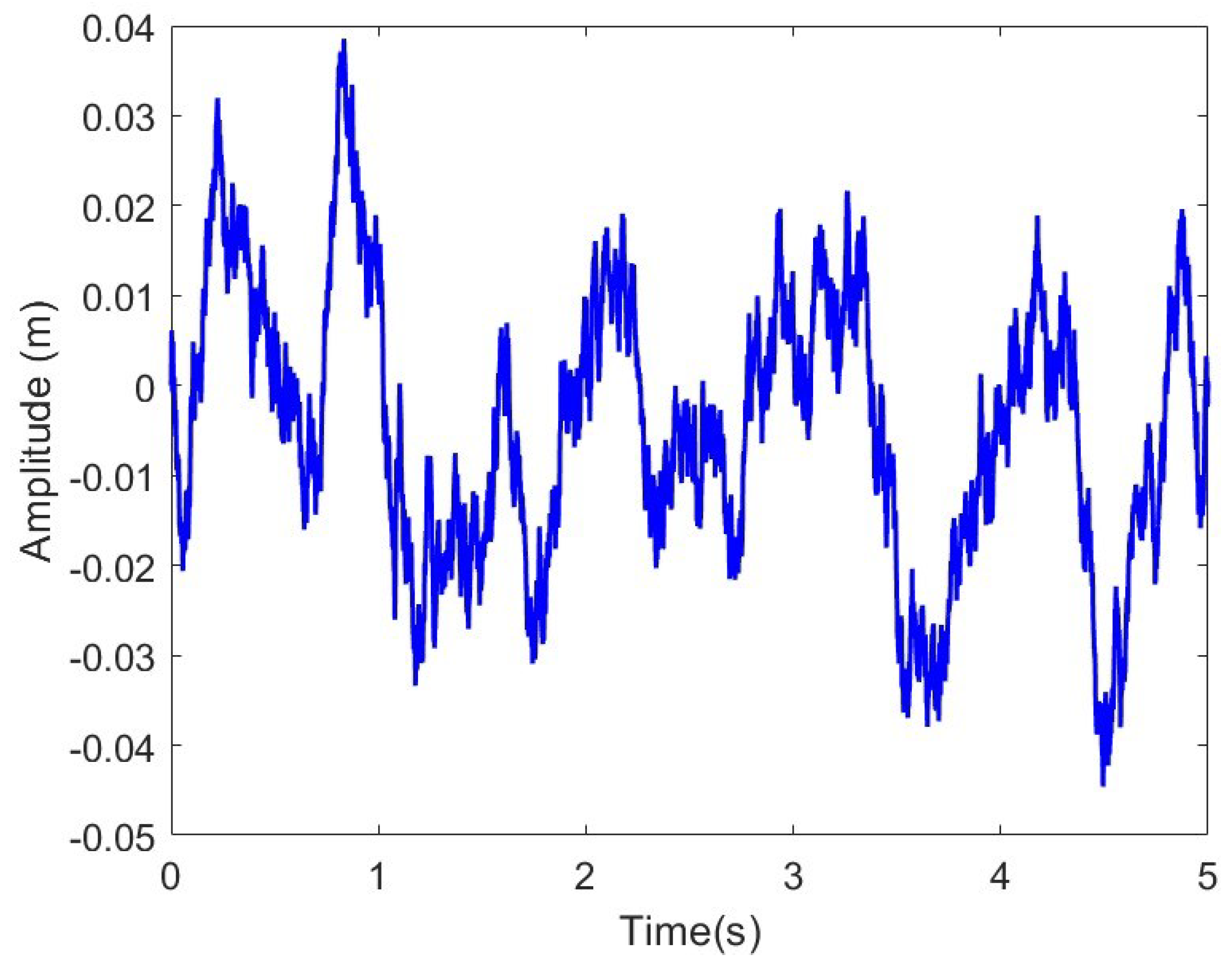
4. Simulation and Results

In this section, the performance of the proposed FONTSM-DOB controller is tested by two simulation cases. The first case is a simulation tracking a step signal, and the second case is a simulation tracking a harmonic signal. Also, the PD-LESO controller proposed in literature [54] and the FONTSM controller proposed in literature [55] will be introduced to compare with the controller of this paper. Both of simulation cases are carried out using MATLAB R2024a/Simulink on a computer featuring a 3.50-GHz Intel Core i5-14600KF CPU running Windows 11. A sampling rate of 1000 Hz, along with the fourth-order Runge–Kutta (ode 4) solver, is utilized.
In the simulation, the quadrotor of the UAM is maintained in a hovering state, with its generated perturbations included in the lumped disturbances of the robotic manipulator system. The gripper at the end of the manipulator is tasked with grasping a cylinder target, as depicted in Figure 1, while tracking a step trajectory and a harmonic trajectory, respectively.
The workspace of the proposed UAM needs to be calculated so as to ensure that the selected desired trajectory is valid. The solution of the working space of the manipulator can be obtained by Monte Carlo method [56] as shown in the following formula:
q i = q i min + q i max q i min · randn ( 0 , 1 )
where randn ( 0 , 1 ) s a normally distributed random function. The bit shape of the end-effector of the aerial manipulator is obtained by substituting the generated random joint angles into the forward kinematics Equation (3). The workspace of the aerial manipulator with 1000 random points is given in Figure 3.

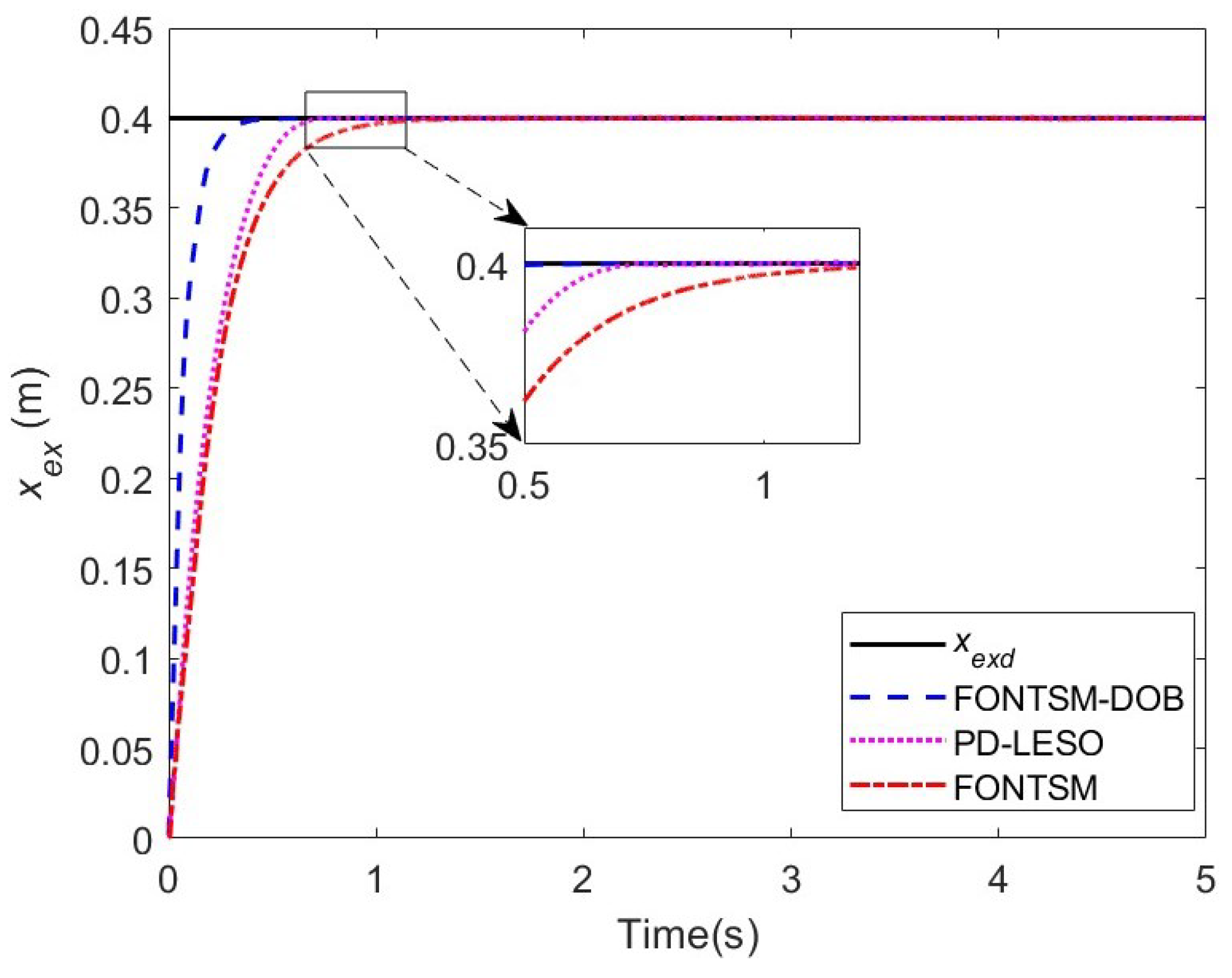
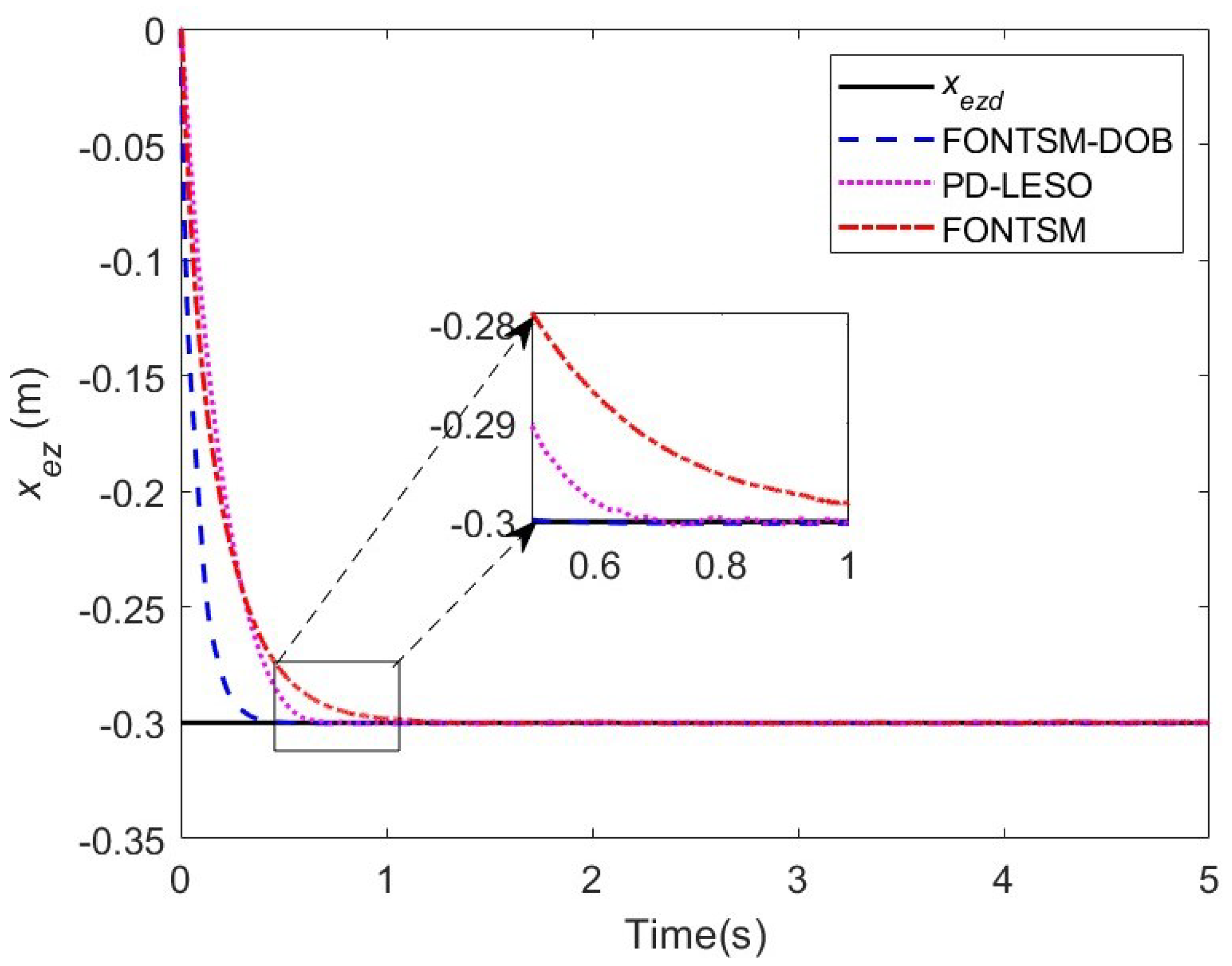
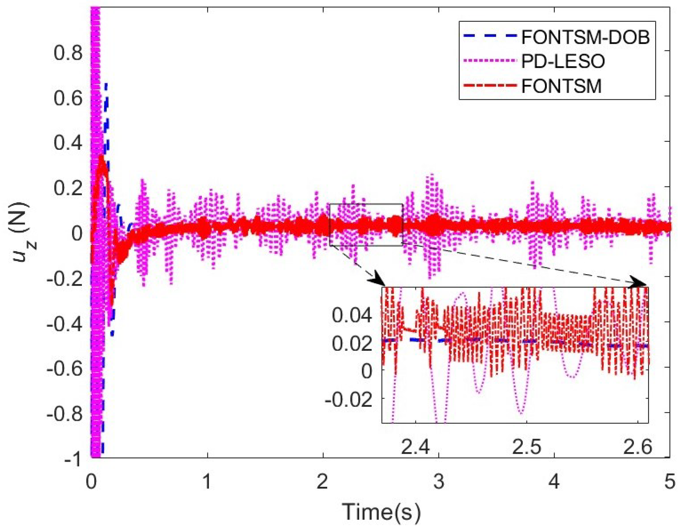
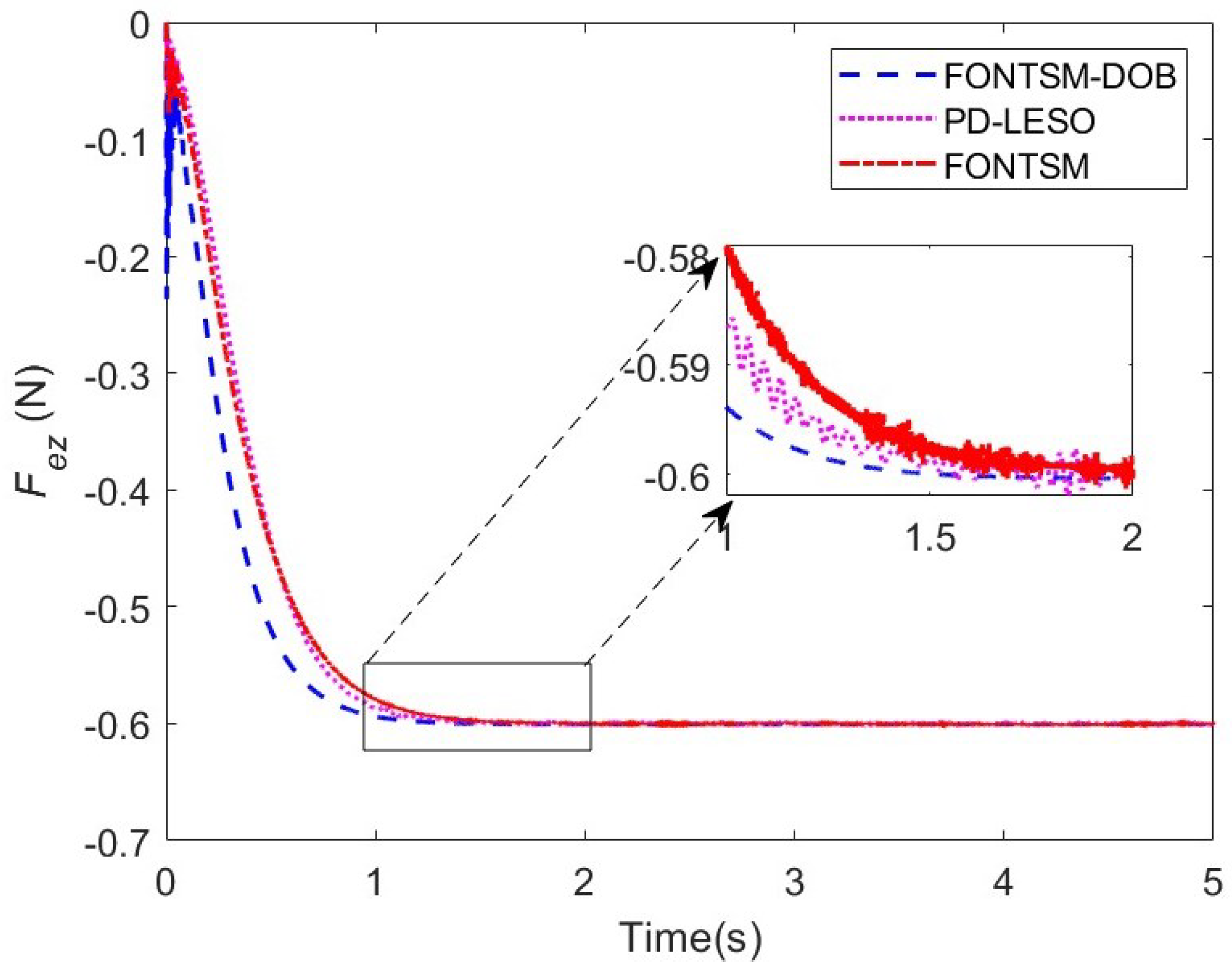
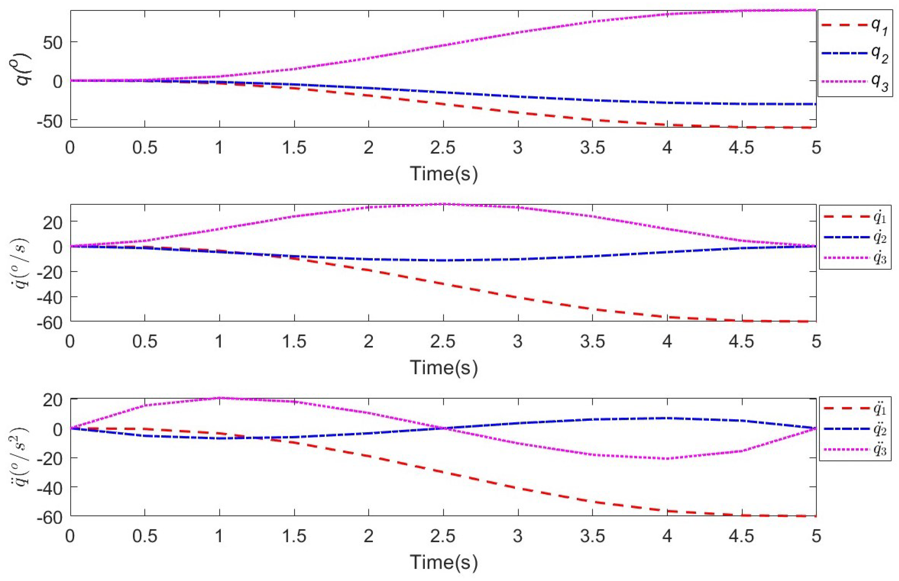
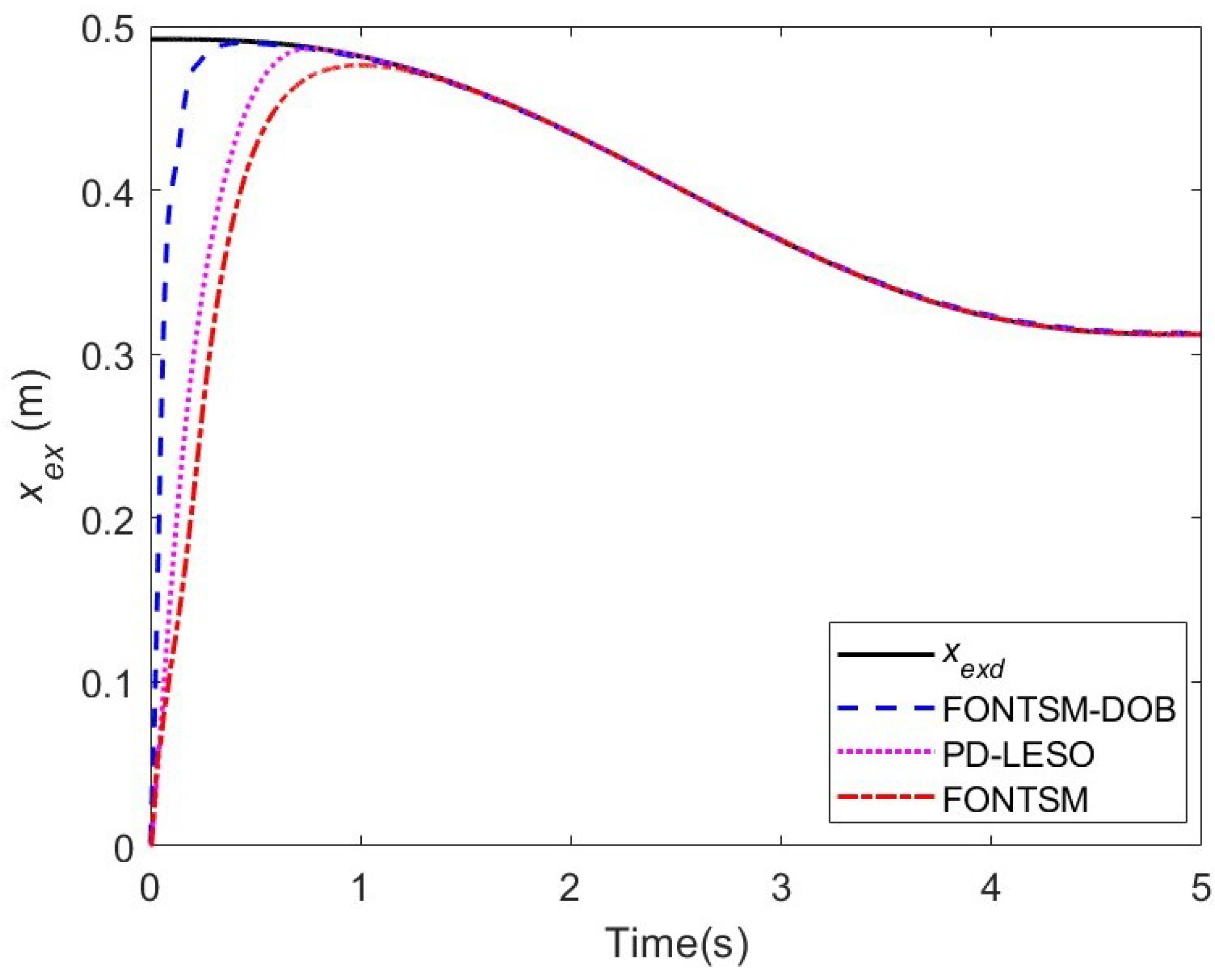
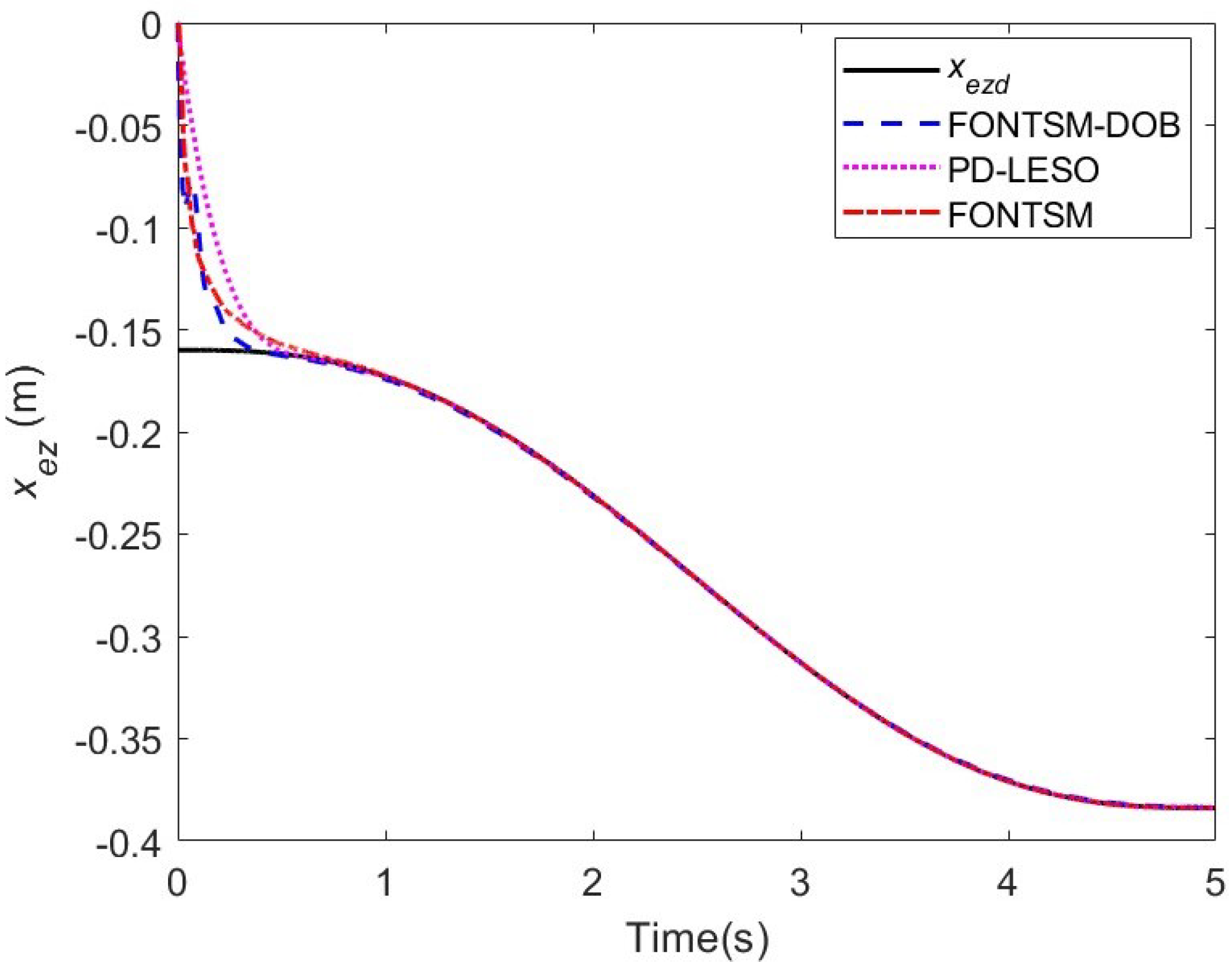
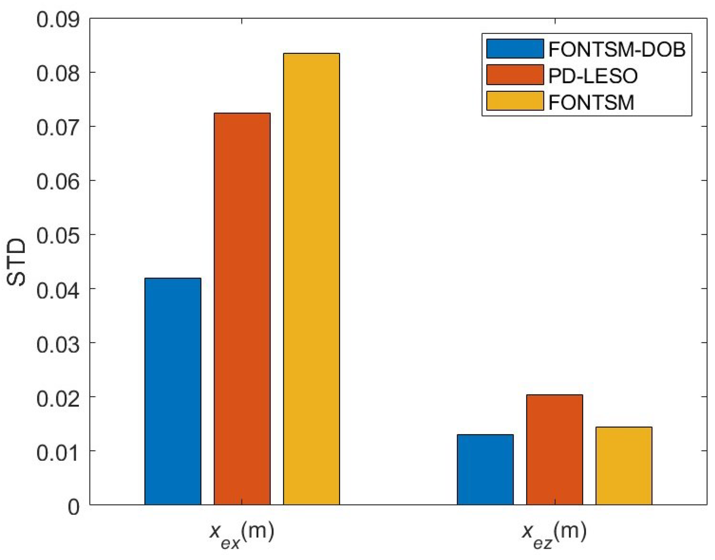
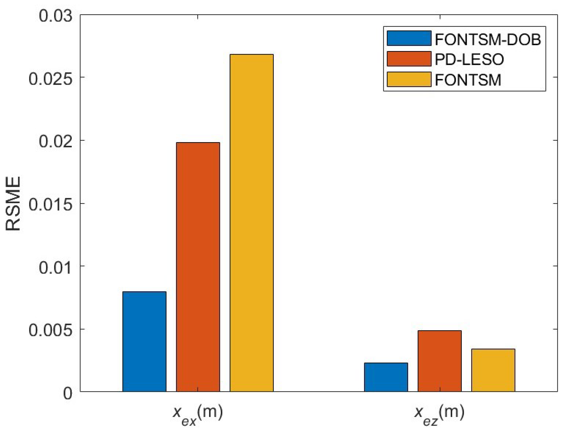
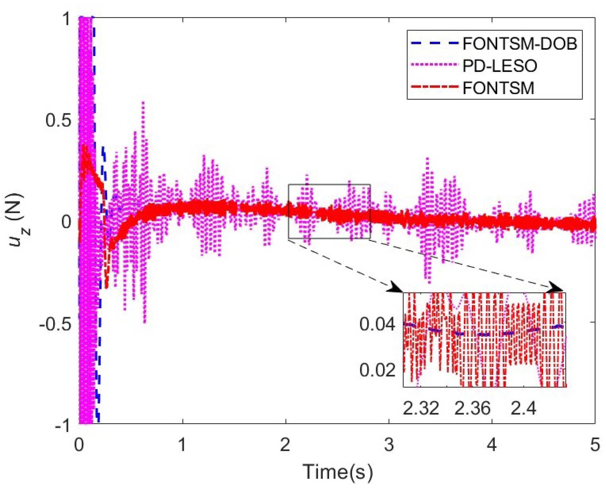
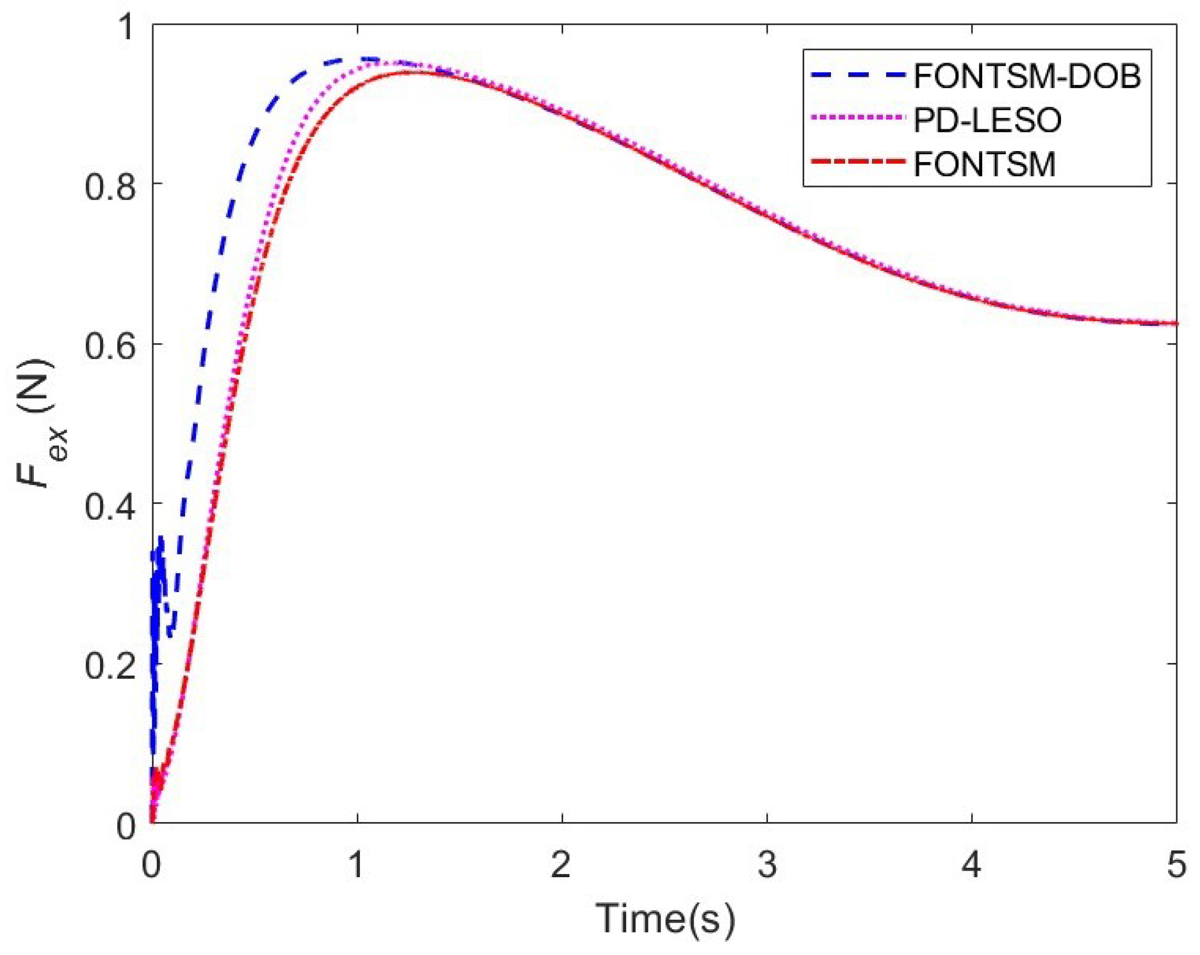
4.1. Case 1: Tracking a Step Signal

The reference signal is set to x exd , x ezd = [ 0.4 m , 0.3 m ] , the initial values of other state quantities are all 0, and the simulation time lasts for 5 s. In the simulation, a random function is added in the x axis and the z axis to simulate the lumped disturbances in the system, as shown in Figure 4, respectively.
The parameters of the three controllers are given in Table 2, and they were obtained by manual empirical methods. Among them, some of the parameters of FONTSM and FONTSM-DOB are consistent, and the explanation of the parameters of PD-LESO can be found in literature [54] and will not be explained here. Another role of this case is to provide the appropriate controller parameters for the next case.
The tracking responses of the aerial manipulator’s end-effector, as illustrated in Figure 5 and Figure 6, offer a comparative evaluation of the performance of the FONTSM-DOB, PD-LESO, and FONTSM controllers. Figure 5 shows the x e x tracking response, highlighting that FONTSM-DOB exhibits superior transient behavior, characterized by a rapid rise time and minimal overshoot. The enlarged view further emphasizes FONTSM-DOB’s capacity to converge quickly to the desired trajectory, showcasing its robust disturbance rejection and precise control capabilities. In contrast, PD-LESO, although effective, demonstrates a slightly longer settling time, while FONTSM shows even greater delays, accompanied by more pronounced steady-state error, which indicates a less effective disturbance rejection. Figure 6 supports these findings in the x e z response, where FONTSM-DOB consistently outperforms the alternatives. It attains the desired state with remarkable speed and minimal oscillation, underscoring its superior transient and steady-state performance. In contrast, PD-LESO, while competent, exhibits slower convergence and a slightly higher overshoot. Additionally, FONTSM’s extended settling time and greater deviation during the transient phase highlight its limitations in robustness and precision.
Figure 7 and Figure 8 depict the control output responses of the aerial robotic arm under the control of the three controllers. The results clearly indicate that FONTSM-DOB exhibits superior transient and steady-state performance compared to the other two controllers. Specifically, FONTSM-DOB achieves rapid stabilization with minimal oscillation, demonstrating its enhanced ability to efficiently manage system dynamics and disturbances. The markedly reduced oscillations and faster convergence in both ux and uz responses highlight FONTSM-DOB’s robust disturbance rejection capabilities and superior control stability. In contrast, PD-LESO and FONTSM exhibit prolonged oscillatory behavior and slower convergence, reflecting their relative inferiority in disturbance mitigation and precision control. These observations underscore FONTSM-DOB as a better choice for high precision and high reliable control in aerial manipulator applications.
Figure 9 and Figure 10 illustrate the force responses under the application of the three impedance controllers. The data reveal that FONTSM-DOB exhibits superior performance in achieving rapid force convergence with minimal overshoot. The magnified views underscore FONTSM-DOB’s effectiveness in attenuating oscillations, thereby ensuring precise impedance regulation and robust interaction with the environment. In comparison, PD-LESO and FONTSM demonstrate longer settling times and more pronounced oscillations, indicative of their relatively lower efficacy in handling the intricate dynamics of aerial manipulators. These results emphasize the advanced capabilities of FONTSM-DOB in enhancing the stability and precision of impedance control in aerial manipulator systems.

4.2. Case 2: Tracks a Harmonic Signal

The initial position of the end-effector of the aerial manipulator is set to x exd 1 , x ezd 1 = [ 0.482 m , 0.160 m ] , the termination position to x exd 2 , x ezd 2 = [ 0.312 m , 0.384 m ] , the initial values of the other state quantities are set to 0, and the simulation time lasts for 5 s. The same lumped disturbances as in Case 1 are added to the manipulator system. First, the joint angles at the time of initiation and termination are computed by Equations (4)–(9), and then the trajectory of the manipulator in the joint space is planned by using fifth-degree polynomials, which is shown below:
q ( t ) = a 0 + a 1 t + a 2 t 2 + a 3 t 3 + a 4 t 4 + a 5 t 5 q ˙ ( t ) = a 1 + 2 a 2 t + 3 a 3 t 2 + 4 a 4 t 3 + 5 a 5 t 4 q ¨ ( t ) = 2 a 2 + 6 a 3 t + 12 a 4 t 2 + 20 a 5 t 3 , s . t . q ( 0 ) = q 0 , q ˙ ( 0 ) = q ˙ 0 , q ¨ ( 0 ) = q ¨ 0 q ( T ) = q T , q ˙ ( T ) = q ˙ T , q ¨ ( T ) = q ¨ T
where a i ( i = 0 , , 5 ) is the factors, T denotes the termination time, T = 5 in the article.
Figure 11 illustrates the planned trajectory of the aerial manipulator’s joint angles using a fifth-degree polynomial. The smooth evolution of joint positions, velocities, and accelerations highlights the efficacy of the trajectory planning method, ensuring minimal jerk and continuous motion, which is critical for maintaining system stability and precision during operation.
The planned sequence of joint angles is substituted into Equation (3) to determine the position variation of the end-effector. It is important to note that the variation in the attitude of the manipulator’s end-effector is not considered in this simulation. Figure 12 illustrates the smooth and precise trajectory of the end-effector within the workspace, demonstrating the manipulator’s effective calculation and accurate trajectory following.
Figure 13 and Figure 14 depict the end-effector tracking responses under the three control strategies. FONTSM-DOB exhibits markedly superior transient performance, characterized by faster rise time, reduced overshoot, and quicker settling time, reflecting its robust dynamic control. However, the initial ripple observed in Figure 14, likely due to intense sliding mode switching, indicates potential chattering and high-frequency oscillations. Conversely, PD-LESO and FONTSM display smoother initial responses but at the cost of slower convergence, highlighting a critical trade-off between aggressive control efficacy and system smoothness, whereas good transient control performance is crucial for high-precision maneuvering tasks.
Further, Figure 15 and Figure 16 provide a comprehensive evaluation of trajectory tracking accuracies under the three controllers, quantified by standard deviation (STD) and root-mean-square error (RMSE). ONTSM-DOB demonstrates remarkable performance, particularly in the x axis, where its STD is 41.97% and 49.67% lower, and its RMSE is 59.94% and 70.36% lower compared to PD-LESO and FONTSM, respectively. In the z axis, FONTSM-DOB also outperforms the other controllers, with its STD being 36.28% and 10.00% lower, and RMSE 53.19 % and 32.73% lower than those of PD-LESO and FONTSM, respectively. These significant reductions in tracking errors underscore the superior precision and robustness of FONTSM-DOB in managing trajectory errors, even under varying dynamic conditions.
Figure 17 and Figure 18 reveal distinct performance characteristics among the outputs of the three controllers. FONTSM-DOB performs well, delivering stable control outputs with minimal oscillations, highlighting its robust disturbance rejection and superior dynamic management. Conversely, PD-LESO exhibits significant high-frequency oscillations, indicative of potential chattering and instability under nonlinear dynamics. FONTSM, while smoother than PD-LESO, still shows greater variability than FONTSM-DOB, suggesting less effective control stability. These findings affirm FONTSM-DOB’s ability as the most reliable choice for precision and robustness in demanding control applications.
The variation in contact force along the X-axis and Z-axis is depicted in Figure 19 and Figure 20. The figures indicate that the FONTSM-DOB controller achieves superior control performance for contact force. However, a sharp oscillation in the contact force is observed during the 0–0.3 s interval, likely due to high-frequency switching on the sliding mode surface. Despite this, the control remains manageable, as the system incorporates an input saturation limit, preventing potential harm to the actuator. This observation underscores the reliability of the FONTSM-DOB controller developed in this study, demonstrating its robustness in practical applications.

5. Conclusions

This article proposed a novel fractional-order nonsingular terminal sliding mode control (FONTSM-DOB) strategy for impedance control in cable-driven aerial manipulators (UAMs) operating under contact conditions with external environments. The developed approach integrates fractional calculus, disturbance observer, and nonsingular terminal sliding mode control Techniques to address the inherent challenges of complex dynamic interactions, external disturbances, and nonlinearities in UAM systems. Simulation results demonstrate that the proposed FONTSM-DOB controller outperforms conventional control methods, such as PD-LESO and FONTSM, in achieving rapid and precise trajectory tracking with minimal oscillations and enhanced robustness against lumped disturbances. The research results demonstrate that the proposed FONTSM-DOB controller significantly enhances the stability, accuracy, and flexibility of the UAM during contact operations with its environment, thereby improving the overall reliability of the UAM. Future work could explore the implementation of this control strategy in experimental setups and extend its application to more complex multi-contact manipulation tasks.

Author Contributions

Conceptualization, L.D. and H.W.; methodology, L.D.; software, T.X.; validation, L.D., D.L. and M.L.; formal analysis, T.X.; investigation, R.M.; resources, D.L.; data curation, M.L.; writing—original draft preparation, L.D.; writing—review and editing, T.X.; visualization, R.M.; supervision, H.W.; project administration, L.D.; funding acquisition, L.D. and M.L. All authors have read and agreed to the published version of the manuscript.

Funding

This research was funded by the National Natural Science Foundation of China (52375101, 52005231), the Social Development Science and Technology Support Project of Changzhou (CE20215050), and Jiangsu University Youth and Blue Project Funding.

Data Availability Statement

The data of simulation can be provided if necessary.

Acknowledgments

Thanks to the anonymous reviewers for their helpful and insightful remarks. In addition, helpful discussions with Xiaofeng Liu from Hohai University and his guidance concerning aircraft designation are gratefully acknowledged.

Conflicts of Interest

The authors declare no conflict of interest.

Abbreviations

The following abbreviations are used in this manuscript:
UAVUnmanned aerial vehicles
UAMUnmanned aerial manipulator
DOFDegree-of-freedom
SMCSliding mode control
TSMTerminal sliding mode
FTSMFast terminal sliding mode
NFTSMNonsingular fast terminal sliding mode
DOBDisturbance observer
IOInteger-order
FOFractional order
FONTSM-DOBFractional order nonsingular terminal sliding mode based on DOB
DHDenavit–Hartenberg

References

  1. Uthayasooriyan, A.; Vanegas, F.; Jalali, A.; Digumarti, K.M.; Janabi-Sharifi, F.; Gonzalez, F. Tendon-Driven Continuum Robots for Aerial Manipulation—A Survey of Fabrication Methods. Drones 2024, 8, 269. [Google Scholar] [CrossRef]
  2. Ramon-Soria, P.; Arrue, B.C.; Ollero, A. Grasp planning and visual servoing for an outdoors aerial dual manipulator. Engineering 2020, 6, 77–88. [Google Scholar] [CrossRef]
  3. Tognon, M.; Chávez, H.A.T.; Gasparin, E.; Sablé, Q.; Bicego, D.; Mallet, A.; Lany, M.; Santi, G.; Revaz, B.; Cortés, J.; et al. A truly-redundant aerial manipulator system with application to push-and-slide inspection in industrial plants. IEEE Robot. Autom. Lett. 2019, 4, 1846–1851. [Google Scholar] [CrossRef]
  4. Phillips-Grafflin, C.; Suay, H.B.; Mainprice, J.; Alunni, N.; Lofaro, D.; Berenson, D.; Chernova, S.; Lindeman, R.W.; Oh, P. From autonomy to cooperative traded control of humanoid manipulation tasks with unreliable communication: Applications to the valve-turning task of the darpa robotics challenge and lessons learned. J. Intell. Robot. Syst. 2016, 82, 341–361. [Google Scholar] [CrossRef]
  5. Ding, L.; Zhu, G.; Li, Y.; Wang, Y. Cable-Driven Unmanned Aerial Manipulator Systems for Water Sampling: Design, Modeling, and Control. Drones 2023, 7, 450. [Google Scholar] [CrossRef]
  6. Kutia, J.R.; Stol, K.A.; Xu, W. Aerial manipulator interactions with trees for canopy sampling. IEEE/ASME Trans. Mechatronics 2018, 23, 1740–1749. [Google Scholar] [CrossRef]
  7. Meng, X.; He, Y.; Han, J. Survey on aerial manipulator: System, modeling, and control. Robotica 2020, 38, 1288–1317. [Google Scholar] [CrossRef]
  8. Xu, W.; Cao, L.; Zhong, C. Review of aerial manipulator and its control. Int. J. Robot. Control Syst. 2021, 1, 308–325. [Google Scholar] [CrossRef]
  9. Zeng, J.; Zhong, H.; Wang, Y.; Fan, S.; Zhang, H. Autonomous control design of an unmanned aerial manipulator for contact inspection. Robotica 2023, 41, 1145–1158. [Google Scholar] [CrossRef]
  10. Liu, J.; Li, Z.; Tian, Y.; Zheng, W. Dynamic modeling and active disturbance rejection control of parallel aerial manipulator system. In Proceedings of the Advances in Guidance, Navigation and Control: Proceedings of 2020 International Conference on Guidance, Navigation and Control, ICGNC 2020, Tianjin, China, 23–25 October 2020; Springer: Berlin/Heidelberg, Germany, 2022; pp. 3281–3293. [Google Scholar]
  11. Ding, L.; Wu, H. Dynamical Modelling and Robust Control for an Unmanned Aerial Robot Using Hexarotor with 2-DOF Manipulator. Int. J. Aerosp. Eng. 2019, 2019, 5483073. [Google Scholar] [CrossRef]
  12. Li, H.; Li, Z.; Liu, J.; Zheng, X.; Yu, X.; Kaynak, O. Adaptive neural network backstepping control method for aerial manipulator based on coupling disturbance compensation. J. Frankl. Inst. 2024, 361, 106733. [Google Scholar] [CrossRef]
  13. Xu, W.; Cao, L.; Peng, B.; Wang, L.; Gen, C.; Liu, Y. Adaptive nonsingular fast terminal sliding mode control of aerial manipulation based on nonlinear disturbance observer. Drones 2023, 7, 88. [Google Scholar] [CrossRef]
  14. Huang, Q.; Dong, C.; Yu, Z.; Chen, X.; Li, Q.; Chen, H.; Liu, H. Resistant compliance control for biped robot inspired by humanlike behavior. IEEE/ASME Trans. Mechatronics 2022, 27, 3463–3473. [Google Scholar] [CrossRef]
  15. Xu, M.; Hu, A.; Wang, H. Image-based visual impedance force control for contact aerial manipulation. IEEE Trans. Autom. Sci. Eng. 2022, 20, 518–527. [Google Scholar] [CrossRef]
  16. Byun, J.; Kim, J.; Eom, D.; Lee, D.; Kim, C.; Kim, H.J. Image-Based Time-Varying Contact Force Control of Aerial Manipulator using Robust Impedance Filter. IEEE Robot. Autom. Lett. 2024, 9, 4854–4861. [Google Scholar] [CrossRef]
  17. Bonilla, I.; Mendoza, M.; Campos-Delgado, D.U.; Hernández-Alfaro, D.E. Adaptive impedance control of robot manipulators with parametric uncertainty for constrained path–tracking. Int. J. Appl. Math. Comput. Sci. 2018, 28, 363–374. [Google Scholar] [CrossRef]
  18. Jin, Z.; Qin, D.; Liu, A.; Zhang, W.a.; Yu, L. Model predictive variable impedance control of manipulators for adaptive precision-compliance tradeoff. IEEE/ASME Trans. Mechatronics 2022, 28, 1174–1186. [Google Scholar] [CrossRef]
  19. Kong, D.; Huang, Q. Impedance force control of manipulator based on variable universe fuzzy control. Actuators 2023, 12, 305. [Google Scholar] [CrossRef]
  20. Sai, H.; Xu, Z.; Li, Y.; Wang, K. Adaptive nonsingular fast terminal sliding mode impedance control for uncertainty robotic manipulators. Int. J. Precis. Eng. Manuf. 2021, 22, 1947–1961. [Google Scholar] [CrossRef]
  21. Lee, J.; Chang, P.H.; Jin, M. Adaptive integral sliding mode control with time-delay estimation for robot manipulators. IEEE Trans. Ind. Electron. 2017, 64, 6796–6804. [Google Scholar] [CrossRef]
  22. Nicolis, D.; Allevi, F.; Rocco, P. Operational space model predictive sliding mode control for redundant manipulators. IEEE Trans. Robot. 2020, 36, 1348–1355. [Google Scholar] [CrossRef]
  23. Zhai, J.; Xu, G. A novel non-singular terminal sliding mode trajectory tracking control for robotic manipulators. IEEE Trans. Circuits Syst. II Express Briefs 2020, 68, 391–395. [Google Scholar] [CrossRef]
  24. Van, M.; Mavrovouniotis, M.; Ge, S.S. An adaptive backstepping nonsingular fast terminal sliding mode control for robust fault tolerant control of robot manipulators. IEEE Trans. Syst. Man, Cybern. Syst. 2018, 49, 1448–1458. [Google Scholar] [CrossRef]
  25. Yi, S.; Zhai, J. Adaptive second-order fast nonsingular terminal sliding mode control for robotic manipulators. ISA Trans. 2019, 90, 41–51. [Google Scholar] [CrossRef]
  26. Zhang, K.; Wang, L.; Fang, X. High-order fast nonsingular terminal sliding mode control of permanent magnet linear motor based on double disturbance observer. IEEE Trans. Ind. Appl. 2022, 58, 3696–3705. [Google Scholar] [CrossRef]
  27. Luo, W.; Liu, S. Disturbance observer based nonsingular fast terminal sliding mode control of underactuated AUV. Ocean. Eng. 2023, 279, 114553. [Google Scholar] [CrossRef]
  28. Wang, Y.; Li, B.; Yan, F.; Chen, B. Practical adaptive fractional-order nonsingular terminal sliding mode control for a cable-driven manipulator. Int. J. Robust Nonlinear Control 2019, 29, 1396–1417. [Google Scholar] [CrossRef]
  29. Mathiyalagan, K.; Sangeetha, G. Second-order sliding mode control for nonlinear fractional-order systems. Appl. Math. Comput. 2020, 383, 125264. [Google Scholar] [CrossRef]
  30. Fei, J.; Wang, H.; Fang, Y. Novel neural network fractional-order sliding-mode control with application to active power filter. IEEE Trans. Syst. Man, Cybern. Syst. 2021, 52, 3508–3518. [Google Scholar] [CrossRef]
  31. Fei, J.; Wang, Z.; Pan, Q. Self-constructing fuzzy neural fractional-order sliding mode control of active power filter. IEEE Trans. Neural Netw. Learn. Syst. 2022, 34, 10600–10611. [Google Scholar] [CrossRef]
  32. Chen, Z.; Wang, X.; Cheng, Y. Adaptive finite-time disturbance observer-based recursive fractional-order sliding mode control of redundantly actuated cable driving parallel robots under disturbances and input saturation. J. Vib. Control 2023, 29, 675–688. [Google Scholar] [CrossRef]
  33. Dou, B.; Yue, X. Disturbance observer-based fractional-order sliding mode control for free-floating space manipulator with disturbance. Aerosp. Sci. Technol. 2023, 132, 108061. [Google Scholar] [CrossRef]
  34. Song, T.; Fang, L.; Zhang, Y.; Shen, H. Recursive terminal sliding mode based control of robot manipulators with a novel sliding mode disturbance observer. Nonlinear Dyn. 2024, 112, 1105–1121. [Google Scholar] [CrossRef]
  35. Suarez, A.; Heredia, G.; Ollero, A. Physical-virtual impedance control in ultralightweight and compliant dual-arm aerial manipulators. IEEE Robot. Autom. Lett. 2018, 3, 2553–2560. [Google Scholar] [CrossRef]
  36. Zhao, J.; Wang, Y.; Wang, D.; Ju, F.; Chen, B.; Wu, H. Practical continuous nonsingular terminal sliding mode control of a cable-driven manipulator developed for aerial robots. Proc. Inst. Mech. Eng. Part I J. Syst. Control Eng. 2020, 234, 1011–1023. [Google Scholar] [CrossRef]
  37. Ding, Y.; Wang, Y.; Chen, B. A practical time-delay control scheme for aerial manipulators. Proc. Inst. Mech. Eng. Part I J. Syst. Control Eng. 2021, 235, 371–388. [Google Scholar] [CrossRef]
  38. Li, B.; Liu, H.; Ahn, C.K.; Gong, W. Optimized intelligent tracking control for a quadrotor unmanned aerial vehicle with actuator failures. Aerosp. Sci. Technol. 2024, 144, 108803. [Google Scholar] [CrossRef]
  39. Belalia, A.; Schouraqui, S. Trajectory tracking of a robot arm using images sequences. Int. J. Comput. Digit. Syst. 2024, 16, 1067–1081. [Google Scholar] [CrossRef]
  40. Cardou, P.; Bouchard, S.; Gosselin, C. Kinematic-sensitivity indices for dimensionally nonhomogeneous jacobian matrices. IEEE Trans. Robot. 2010, 26, 166–173. [Google Scholar] [CrossRef]
  41. Wang, Y.; Zhang, R.; Ju, F.; Zhao, J.; Chen, B.; Wu, H. A light cable-driven manipulator developed for aerial robots: Structure design and control research. Int. J. Adv. Robot. Syst. 2020, 17, 1729881420926425. [Google Scholar] [CrossRef]
  42. Ding, L.; Liu, K.; Zhu, G.; Wang, Y.; Li, Y. Adaptive robust control via a nonlinear disturbance observer for cable-driven aerial manipulators. Int. J. Control. Autom. Syst. 2023, 21, 604–615. [Google Scholar] [CrossRef]
  43. Ding, L.; Ma, R.; Wu, Z.; Qi, R.; Ruan, W. Optimal Joint Space Control of a Cable-Driven Aerial Manipulator. CMES-Comput. Model. Eng. Sci. 2023, 135, 441–464. [Google Scholar] [CrossRef]
  44. Naceri, A.; Schumacher, T.; Li, Q.; Calinon, S.; Ritter, H. Learning optimal impedance control during complex 3D arm movements. IEEE Robot. Autom. Lett. 2021, 6, 1248–1255. [Google Scholar] [CrossRef]
  45. Yang, C.; Huang, D.; He, W.; Cheng, L. Neural control of robot manipulators with trajectory tracking constraints and input saturation. IEEE Trans. Neural Netw. Learn. Syst. 2020, 32, 4231–4242. [Google Scholar] [CrossRef] [PubMed]
  46. Li, G.; Chen, X.; Yu, J.; Liu, J. Adaptive neural network-based finite-time impedance control of constrained robotic manipulators with disturbance observer. IEEE Trans. Circuits Syst. II Express Briefs 2021, 69, 1412–1416. [Google Scholar] [CrossRef]
  47. He, T.; Wu, Z. Neural network disturbance observer with extended weight matrix for spacecraft disturbance attenuation. Aerosp. Sci. Technol. 2022, 126, 107572. [Google Scholar] [CrossRef]
  48. Van, M.; Ge, S.S. Adaptive fuzzy integral sliding-mode control for robust fault-tolerant control of robot manipulators with disturbance observer. IEEE Trans. Fuzzy Syst. 2020, 29, 1284–1296. [Google Scholar] [CrossRef]
  49. Della Santina, C.; Truby, R.L.; Rus, D. Data–driven disturbance observers for estimating external forces on soft robots. IEEE Robot. Autom. Lett. 2020, 5, 5717–5724. [Google Scholar] [CrossRef]
  50. Li, S.; Yang, J.; Chen, W.H.; Chen, X. Disturbance Observer-Based Control: Methods and Applications; CRC Press: Boca Raton, FL, USA, 2014. [Google Scholar]
  51. Yao, Y.; Ding, L.; Wang, Y. Fractional-Order Nonsingular Terminal Sliding Mode Control of a Cable-Driven Aerial Manipulator Based on RBF Neural Network. Int. J. Aeronaut. Space Sci. 2024, 25, 759–771. [Google Scholar] [CrossRef]
  52. Guo, Y.; Ma, B.; Chen, L.; Wu, R. Adaptive sliding mode control for a class of Caputo type fractional-order interval systems with perturbation. IET Control Theory Appl. 2017, 11, 57–65. [Google Scholar] [CrossRef]
  53. Karami-Mollaee, A.; Tirandaz, H.; Barambones, O. On dynamic sliding mode control of nonlinear fractional-order systems using sliding observer. Nonlinear Dyn. 2018, 92, 1379–1393. [Google Scholar] [CrossRef]
  54. Gao, J.; Liang, X.; Chen, Y.; Zhang, L.; Jia, S. Hierarchical image-based visual serving of underwater vehicle manipulator systems based on model predictive control and active disturbance rejection control. Ocean. Eng. 2021, 229, 108814. [Google Scholar] [CrossRef]
  55. Raoufi, M.; Delavari, H. Experimental implementation of a novel model-free adaptive fractional-order sliding mode controller for a flexible-link manipulator. Int. J. Adapt. Control Signal Process. 2021, 35, 1990–2006. [Google Scholar] [CrossRef]
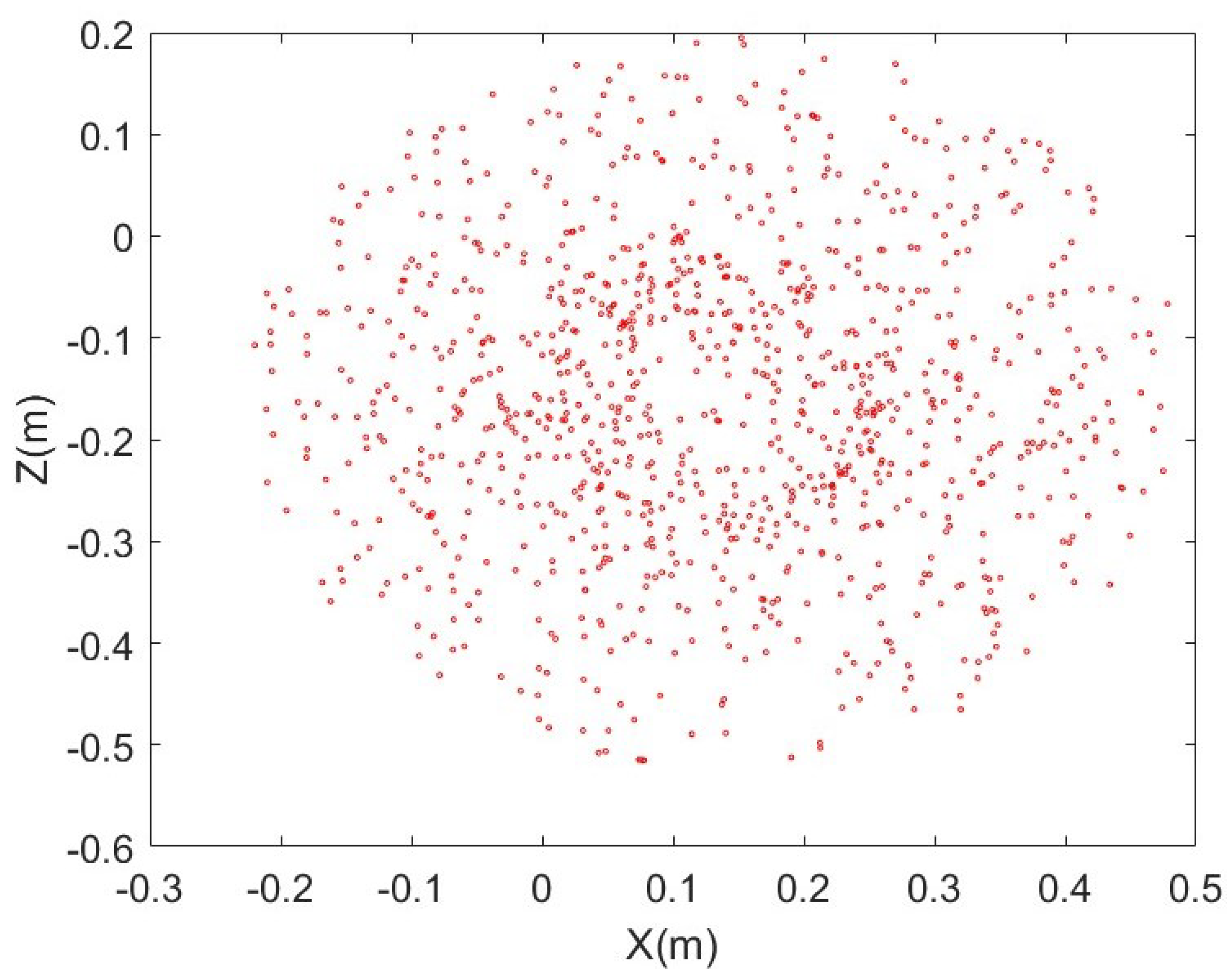
  56. Chaudhury, A.N.; Ghosal, A. Optimum design of multi-degree-of-freedom closed-loop mechanisms and parallel manipulators for a prescribed workspace using Monte Carlo method. Mech. Mach. Theory 2017, 118, 115–138. [Google Scholar] [CrossRef]
Figure 1. UAM’s scheme.
Fractalfract 08 00579 g001
Figure 2. Architecture of FONTSM-DOB.
Fractalfract 08 00579 g002
Figure 3. Workspace of the aerial manipulator using the Monte Carlo method.
Fractalfract 08 00579 g003
Figure 4. Curve of the lumped disturbances.
Fractalfract 08 00579 g004
Figure 5. Response of x e x in Case 1.
Fractalfract 08 00579 g005
Figure 6. Response of x e z in Case 1.
Fractalfract 08 00579 g006
Figure 7. Response of u x in Case 1.
Fractalfract 08 00579 g007
Figure 8. Response of u z in Case 1.
Fractalfract 08 00579 g008
Figure 9. Response of F e x in Case 1.
Fractalfract 08 00579 g009
Figure 10. Response of F e z in Case 1.
Fractalfract 08 00579 g010
Figure 11. Trajectory of the aerial manipulator’s joint angles in joint-space.
Fractalfract 08 00579 g011
Figure 12. Trajectory of the aerial manipulator’s end-effector in workspace.
Fractalfract 08 00579 g012
Figure 13. Response of x e x in Case 2.
Fractalfract 08 00579 g013
Figure 14. Response of x e z in Case 2.
Fractalfract 08 00579 g014
Figure 15. STD of the tracking trajectories in Case 2.
Fractalfract 08 00579 g015
Figure 16. RSME of the tracking trajectories in Case 2.
Fractalfract 08 00579 g016
Figure 17. Response of u x in Case 2.
Fractalfract 08 00579 g017
Figure 18. Response of u z in Case 2.
Fractalfract 08 00579 g018
Figure 19. Response of F e x in Case 2.
Fractalfract 08 00579 g019
Figure 20. Response of F e z in Case 2.
Fractalfract 08 00579 g020
Table 1. DH parameters of the cable-driven manipulator.
LinkLink Length a i Link Twist α i Joint Offset d i Joint Angle q i
10.1200 q 1
20.1200 q 2
30.1200 q 3
Table 2. Control parameters of the three controllers.
ControllerParameters
PD-LESO ω o = 500 , ω c = 800
FONTSM k x = k z = 800 , γ x = γ z = 0.5 , β x = β z = 0.5 , η x = η z = 1000 , h x = h z = 5000
FONTSM-DOB l x = l z = 200 , k x = k z = 1000 , γ x = γ z = 0.5 , β x = β z = 0.5 , η x = η z = 1000 , h x = h z = 5000
Disclaimer/Publisher’s Note: The statements, opinions and data contained in all publications are solely those of the individual author(s) and contributor(s) and not of MDPI and/or the editor(s). MDPI and/or the editor(s) disclaim responsibility for any injury to people or property resulting from any ideas, methods, instructions or products referred to in the content.

