Extinction Dynamics and Equilibrium Patterns in Stochastic Epidemic Model for Norovirus: Role of Temporal Immunity and Generalized Incidence Rates

Abstract

Norovirus is a leading global cause of viral gastroenteritis, significantly affecting mortality, morbidity, and healthcare costs. This paper develops and analyzes a stochastic $\mathsf{S}\mathsf{E}\mathsf{I}\mathsf{Q}\mathsf{R}$ epidemic model for norovirus dynamics, incorporating temporal immunity and a generalized incidence rate. The model is proven to have a unique positive global solution, with extinction conditions explored. Using Khasminskii’s method, the model’s ergodicity and equilibrium distribution are investigated, demonstrating a unique ergodic stationary distribution when ${\widehat{\mathcal{R}}}_s>1$. Extinction occurs when ${\mathcal{R}}_0^E<1$. Computer simulations confirm that noise level significantly influences epidemic spread.

1. Introduction

Norovirus, often named Norwalk virus and typically known as the winter vomiting illness, ranks as the major cause of gastroenteritis. Acute viral gastroenteritis is still a prevalent worldwide epidemic. Though they come from different viral families, human noroviruses (NoVs) have achieved much interest in the past twenty years. NoV is mostly spread via the fecal–oral pathway, which involves coming into touch with human feces. It is widely believed that vomiting can also spread the virus. NoV can spread directly or indirectly through consuming contaminated food or water, coming into contact with contaminated surfaces (fomites), and other means resulting from these two main sources [1]. The proportional impact of each transmission pathway is up for discussion; however, it is commonly known that the NoV group contributes considerably to the worldwide burden of foodborne infections [2,3].

The following three meals are frequently linked to occasional episodes and outbreaks of viral gastroenteritis [3]:

A₁:

Molluscan shellfish become affected throughout the packing process.

A₂:

Fresh products are polluted during collecting, manufacturing, or packaging.

A₃:

Infection may occur in the preparation of ready-for-consumption foods.

It has been noted that poor hygiene practices among those working in the food preservation industries have a significant role in viral spread. Numerous factors increase the likelihood of contamination by diseased food workers. These include the phase of clinical illness, which affect the amount of virus shed, as well as hygiene and health habits, the efficacy of inactivation of the virus, persistence, the ease of virus transmission, and other numerous individual traits. The two most prominent sources and recipients of norovirus are contaminated hands and, to some extent, infected surfaces [4].

Various variables are responsible for norovirus transmission and for the subsequent infection. A significant number of cases were noticed during the nonsummer months, illustrating the seasonality behavior of norovirus [5]. Environmental variables and population behaviors are responsible for seasonal variance. Norovirus, for example, spreads very fast in low temperatures and may be aggravated by increasing rainfall [6,7]. Several population characteristics can impact the severity of NoV outbreaks. The condition affects individuals irrespective of their ages but is more common in children who are less than or equal to five [8]. Serological investigations show that the initial infection due to NoV usually occurs during the early years of childhood. Individuals with weaker immune systems, such as the elderly, are more likely to suffer from serious health conditions and may even die [9,10]. Consequently, while infection is normally self-restricting in people with good health, the consequences can be disastrous for some high-risk groups. Studies have demonstrated that these groupings may shed the virus for a significantly longer period of time, potentially extending an outbreak [10,11,12,13].

The tools of mathematical modeling are crucial to comprehend the transmission of epidemic diseases and forecast the efficacy of novel control strategies [14,15]. These models find a compromise between biological correctness in representing the natural course of infections and the strength of their data linkages. NoV models were created at various scales, from outbreak to populace, and yielded various estimations for the threshold parameters. Environmental influences continue to have an important role in biological phenomena and real-world systems. Environmental factors significantly influence the propagation of norovirus outbreaks [16]. Due to the unpredictability of contact between individuals and other demographic characteristics, the spread of an epidemic is essentially unpredictable. Consequently, the environment’s variations and randomness have a greater impact on the future behavior of the infection. Norovirus infection is a perfect illustration of an epidemic whose behavior could be drastically affected by contaminated food, water, and person-to-person contact.

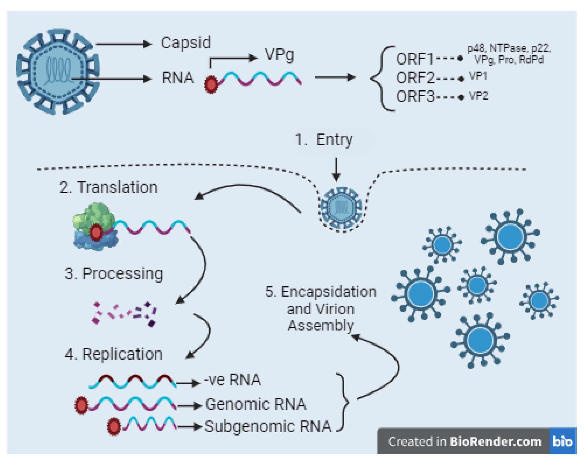
1.1. Structure and Life Cycle of Norovirus

Noroviruses, notorious for causing widespread outbreaks of gastroenteritis, are part of the Caliciviridae family. These viruses are uniquely efficient at spreading and causing illness. Even minimal exposure to the virus can lead to infection, with individuals capable of emitting large quantities of the virus through various means, including direct contact and environmental contamination. Understanding the norovirus structure and life cycle enables the development of more accurate and detailed mathematical models (Figure 1). These models can predict the virus’s spread, taking into account factors like the infectious dose, the rate of virus shedding, and the duration of infectivity, which are directly influenced by the virus’s biological characteristics. The genetic structure of the norovirus plays a crucial role in its infectivity and interaction with the human body. Its genome, a single-stranded RNA about 7.5 kb long, encodes three main proteins through open reading frames (ORFs). These include a large nonstructural polyprotein, and two structural proteins, VP1 and VP2, which together form the virus’s protective capsid. This capsid is key to the virus’s ability to bind to host cells and initiate infection.

Despite the robust immune response in healthy individuals, which typically leads to the resolution of the infection, noroviruses can pose severe risks to certain groups. The elderly, young children, and those with compromised immune systems are particularly vulnerable to more severe complications. The emergence of new norovirus strains, believed to be linked to genetic differences, has heightened concerns about the impact on these susceptible populations. Recent advancements in cultivating noroviruses in cell cultures have opened new pathways for studying these genetic variations and developing potential vaccines, particularly targeting the structural protein VP1.

• Entry: The norovirus capsid, comprised of structural proteins VP1 and VP2, binds to the host cell surface via interactions with histo-blood group antigens (HBGAs), facilitating viral entry. The capsid is then internalized and disassembled, releasing the positive-sense RNA ((+)RNA)) genome into the cytoplasm.
• Translation and Processing of the Viral Genome: The (+)RNA genome is translated into a polyprotein by host cell mechanisms, a process initiated by the nonstructural protein VPg, which attaches to the 5’ end of the RNA. This polyprotein is subsequently cleaved into six nonstructural proteins by the virus-encoded protease, Pro.
• Replication: The (+)RNA serves as a template for the synthesis of complementary negative sense RNAs, which are then used to produce new copies of genomic and subgenomic (+)RNAs. These steps facilitate the replication of the viral genome and the production of structural protein-encoding RNAs.
• Subgenomic RNA Production: Subgenomic (+)RNAs, which specifically contain ORF2 and ORF3, are synthesized to produce the structural proteins VP1 and VP2.
• Encapsidation and Virion Assembly: Newly synthesized genomic and subgenomic (+)RNAs are packaged into new virions through a process of encapsidation, with the assembly of the capsid proteins VP1 and VP2 around the RNA genome. The newly assembled virions are released from the host cell to initiate further infections. The exact mechanism of virion release remains an area of ongoing research.

1.2. Motivation

Environmental variations have a substantial impact on parasite transmission and persistence. Stochastic variables have a significant influence on epidemics since fluctuation may be stochastic but strongly autocorrelated, mimicking the recent past (red noise), or uncorrelated and random with the past (white noise). These noises may be estimated theoretically by transforming aerial photos into a probability density function of photons [17,18,19,20].

To model the dynamics of infectious diseases in mathematical terms, generally, two types of approaches are employed: stochastic and deterministic modeling. It is widely accepted that the tools of stochastic modeling are much more beneficial for modeling biological phenomena, as they reflect the dynamics of the underlying problem realistically compared to deterministic modeling [21,22,23]. Further, simulating a stochastic model several times allows for the construction of a distribution for expected outputs, like the size of infected persons at time t, which results in more useful outputs than deterministic models. Unlike deterministic models, which provide a single result regardless of previous tests, stochastic models provide a variety of options. References [24,25] show that several deterministic epidemiological models have been suggested to explore NoV virus dynamics. Most of the NoV transmission models use the compartmental approach to modeling, where the population is divided into various disease stages. Typically, this stratification divides the population into three basic groups, susceptible ($\mathsf{S}$), infected ($\mathsf{I}$), and recovered ($\mathsf{R}$), indicated as $\mathsf{S}\mathsf{I}\mathsf{R}$. Other viral epidemic models include an additional compartment called the exposed or latent class ($\mathsf{E}$). Including the latent compartment in the NoV model is critical for evaluating the efficacy of infection control strategies [26,27]. Merely a few researchers have studied the changing behavior of NoV models, including the inherent noises [25]. To the authors’ knowledge, no previous research has used mathematical modeling to explore NoV transmission through polluted water or food while considering environmental fluctuations. This work focuses on the exploration of NoV dynamics, considering stochastic disturbances. We assume that the immunity is temporary, and that the person may be infected again with the virus. Further, most of the authors use the bilinear incidence rate, whereas this study considers the generalized incidence of the disease, making the problem more realistic and complex. This work provides a theoretical foundation for understanding chronic infectious diseases globally, particularly norovirus, and emphasizes techniques for constructing Lyapunov functions in nonlinear stochastic epidemic models.

1.3. Contribution

In this research, we present a comprehensive analysis of norovirus (NoV) dynamics through the development of a novel stochastic model that incorporates a general incidence function and considers temporary immunity, allowing for the possibility of reinfection. This model, detailed in Section 2, is particularly innovative for its realistic representation of disease spread mechanisms.

Section 3 of our study is devoted to establishing the mathematical foundations of our model. Here, we prove the existence and uniqueness of a positive global solution, confirming the model’s applicability to real-world epidemic scenarios. Following this, in Section 4, we delve into the conditions under which NoV can exhibit exponential extinction. This analysis is crucial for identifying key parameters that could potentially be targeted in disease control strategies.

Our investigation continues in Section 5, where we explore the necessary conditions for the emergence of an ergodic stationary distribution. This part of the study highlights the long-term stability and behavior of the disease under stochastic influences, including environmental fluctuations. The theoretical insights derived from these sections are empirically tested through numerical simulations as reported in Section 6. These simulations not only validate our theoretical constructs but also demonstrate their practical relevance in predicting and managing NoV outbreaks.

The study concludes in Section 7, where we summarize our findings and discuss their implications for public health policy and epidemic modeling. We also propose potential avenues for future research, focusing on the further development of stochastic models to better understand infectious disease dynamics under varying environmental and demographic conditions. This comprehensive approach underscores the significance of our contributions to the field of epidemiological modeling.

2. Norovirus Dynamics: A Mathematical Approach

Norovirus, known for its high contagious rate, is a pathogen that can cause gastroenteritis, an inflammatory illness attacking the intestines and stomach. Modeling and understanding the spread of an epidemic disease, such as norovirus, is possible using compartmental models.

The study of epidemic models is strongly dependent on knowing the incidence rate of the underlying infectious illnesses. Classical epidemic models commonly employ bilinear incidence rates, which are developed under the premise of homogeneous mixing [28,29,30]. It is experimentally observed that the rate of incidence of the disease should be an increasing function of the parasites the shape of the function should be sigmoidal (for instance, see [31,32]). Keeping in view the importance of the incidence function in disease dynamics, Anderson and May introduced the saturated incidence ${\displaystyle \frac{\alpha SI}{1+\beta S}}$ [33]; ref. [34] formulated the Beddington–DeAngelis type of incidence function ${\displaystyle \frac{\beta xv}{1+mx+nv}}$ in describing HIV epidemic; and similarly, for elaborating the impact of media in disease spread, Caraballo et al. [35] used a different type of incidence rate ${\beta }_1-{\displaystyle \frac{{\beta }_{2}I}{m+I}}$. Motivated by the above and considering the severity of the NoV infection, we formulate the following system of DEs while using the generalized incidence rate

$$\left\{\begin{array}{c}{\displaystyle \frac{d\mathsf{S}\left(t\right)}{dt}}=\mathrm{\Pi }-\mathsf{S}\left(t\right)f\left(\mathsf{I}\left(t\right)\right)-\lambda \mathsf{S}\left(t\right),\hfill \\ {\displaystyle \frac{d\mathsf{E}\left(t\right)}{dt}}=\mathsf{S}\left(t\right)f\left(\mathsf{I}\left(t\right)\right)-(\lambda +\epsilon +{\delta }_1)\mathsf{E}\left(t\right),\hfill \\ {\displaystyle \frac{d\mathsf{I}\left(t\right)}{dt}}=\epsilon \mathsf{E}\left(t\right)-(\lambda +\alpha +{\delta }_2)\mathsf{I}\left(t\right),\hfill \\ {\displaystyle \frac{d\mathsf{Q}\left(t\right)}{dt}}={\delta }_1\mathsf{E}\left(t\right)+{\delta }_{2}I\left(t\right)-(\lambda +\alpha +\gamma )\mathsf{Q}\left(t\right),\hfill \\ {\displaystyle \frac{d\mathsf{R}\left(t\right)}{dt}}=\gamma \mathsf{Q}\left(t\right)-\lambda \mathsf{R}\left(t\right).\hfill \end{array}\right.$$

(1)

The descriptions of various parameters and compartments of the model are depicted in

Table 1. Illustration of the parameters used in model (1).

Parameters	Meaning
$\mathrm{\Pi }$	The immigration or birth rate of susceptible population
$\beta$	The disease transmission rate for exposing disease
$\lambda$	The Natural death rate
$\epsilon$	The rate of infected from exposed class
$\alpha$	The rate of mortality of infected and quarantined individuals because of illness
${\delta }_1$	Rate of quarantine from exposed individuals
${\delta }_2$	Rate of quarantine from infectious individuals
$\gamma$	Rate of recovered from quarantined individuals
$\mathsf{S}\left(t\right)$	The susceptible class
$\mathsf{E}\left(t\right)$	The exposed compartment
$\mathsf{I}\left(t\right)$	The infected individuals
$\mathsf{Q}\left(t\right)$	Quarantined population
$\mathsf{R}\left(t\right)$	People recovered from the infection

. By following the standard method of next-generation matrix, we obtain the expression for the threshold parameter as follows:

$$\begin{array}{c}\hfill {\mathcal{R}}_0^D={\displaystyle \frac{\mathrm{\Pi }\epsilon f^{\prime }\left(0\right)}{\lambda (\lambda +\epsilon +{\delta }_1)(\lambda +\alpha +{\delta }_2)}}.\end{array}$$

Following the results proved in [36], we have the following important assertions about the stability of the system:

• For ${\mathcal{R}}_0^D<1$, model (1) has one and only one fixed point (called the disease-free equilibrium (DFE)), which is locally and globally asymptotically stable.
• A unique stable endemic equilibrium of system (1) exists when ${\mathcal{R}}_0^D>1$.

Noise pollution causes oscillations in the system’s parameters (1), causing them to oscillate around the average position. As a result, many scholars have investigated the role of stochastic variables in infectious disease models, specifically in exploring the dynamic behavior of stochastic systems with generalized rates of incidence [22,23,35]. Fan et al. [37] proposed a stochastic model with delays inside the SIR framework, including a general rate of infection with short-term immunity. By using the strong rule of large numbers, they found sufficient criteria for the mean persistence and extinction. Fatini et al. [38] used a parameter perturbation approach to analyze the equilibrium distributions of a more generalized SIRS system. The study found that disease extinction occurs when ${\mathcal{R}}_0^s<1$, but the epidemic persists when ${\mathcal{R}}_0^s>1$ and at the same time, the term $\beta$ oscillates around the mean value. Liu et al. [39] explored the dynamic behavior of an SIRS stochastic system with nonlinear incidence and logistic growth. They constructed an appropriate Lyapunov function for the model and obtained conditions ensuring the ergodicity and positivity of the solution to the underlying stochastic model.

Given the importance of the incidence function in capturing the dynamics of infectious diseases, this work seeks to broaden the aforementioned principles to investigate the latent characteristics of norovirus. The governing equations illustrating the spread of NoV use the $\mathsf{S}\mathsf{E}\mathsf{I}\mathsf{Q}\mathsf{R}$ model framework, using similar approaches utilized by Zhang et al. [40]. To update the model from deterministic to stochastic, we consider the environmental fluctuations in the form of white Brownian noises, which have a direct dependency on the epidemic compartments $\mathsf{S}$, $\mathsf{E}$, $\mathsf{I}$, $\mathsf{Q}$, and $\mathsf{R}$. Further, such randomness will surely affect the ordinary derivatives ${\displaystyle \frac{d\mathsf{S}}{dt}}$, ${\displaystyle \frac{d\mathsf{E}}{dt}}$, ${\displaystyle \frac{d\mathsf{I}}{dt}}$, ${\displaystyle \frac{d\mathsf{Q}}{dt}}$, and ${\displaystyle \frac{d\mathsf{R}}{dt}}$ in system (1). By including this randomness in the ODE model, we have the following stochastic model:

$$\left\{\begin{array}{c}d\mathsf{S}\left(t\right)=\left[\mathrm{\Pi }-\mathsf{S}\left(t\right)f\left(\mathsf{I}\right(t\left)\right)-\lambda \mathsf{S}\left(t\right)\right]dt+{\eta }_1\mathsf{S}\left(t\right)d{\mathsf{W}}_1\left(t\right),\hfill \\ d\mathsf{E}\left(t\right)=[\mathsf{S}\left(t\right)f\left(\mathsf{I}\left(t\right)\right)-(\lambda +\epsilon +{\delta }_1)\mathsf{E}\left(t\right)]dt+{\eta }_2\mathsf{E}\left(t\right)d{\mathsf{W}}_2\left(t\right),\hfill \\ d\mathsf{I}\left(t\right)=[\epsilon \mathsf{E}\left(t\right)-(\lambda +\alpha +{\delta }_2)\mathsf{I}\left(t\right)]dt+{\eta }_3\mathsf{I}\left(t\right)d{\mathsf{W}}_3\left(t\right),\hfill \\ d\mathsf{Q}\left(t\right)=[{\delta }_1\mathsf{E}\left(t\right)+{\delta }_{2}I\left(t\right)-(\lambda +\alpha +\gamma )\mathsf{Q}\left(t\right)]dt+{\eta }_4\mathsf{Q}\left(t\right)d{\mathsf{W}}_4\left(t\right),\hfill \\ d\mathsf{R}\left(t\right)=[\gamma \mathsf{Q}\left(t\right)-\lambda \mathsf{R}\left(t\right)]dt+{\eta }_5\mathsf{R}\left(t\right)d{\mathsf{W}}_5\left(t\right).\hfill \end{array}\right.$$

(2)

Here are the independent functions: ${\mathsf{W}}_i\left(t\right)$ denotes the standard one-dimensional Brownian motions satisfying the conditions ${\mathsf{W}}_i\left(0\right)=0$, where each ${\eta }_i^2>0$ stands for the intensity of the environmental noise, and $i=1,\cdots ,5$. We presume that the contacts between the susceptible individuals and the infected individuals are given by $f(·)$, called the incidence of the disease, fulfilling the following given assumptions:

(A1)

$f(·)\in C^1({\mathbb{R}}_{+},{\mathbb{R}}_{+})$ with increasing property (i.e., $f^{\prime }\left(\mathsf{I}\right)>0$) and $f\left(0\right)=0$ $\forall 0\le \mathsf{I}$;

(A2)

The function ${\displaystyle \frac{f\left(\mathsf{I}\right)}{\mathsf{I}}}$ is either constant or monotonic decreasing over the interval $(0,\infty )$ and ${\displaystyle \frac{f\left(\mathsf{I}\right)}{f^{\prime }\left(\mathsf{I}\right)}}>I$ $\forall \mathsf{I}\in {\mathbb{R}}_{+}$.

Assumption (A2) further ensures that $f\left(\mathsf{I}\right)>\mathsf{I}{f}^{\prime }\left(0\right),\forall 0<\mathsf{I}$.

Assumption (A2): The function $f\left(I\right)$ is a concave increasing function over the interval $(0,\infty )$, ensuring that

$$I{f}^{\prime }\left(I\right)\le f\left(I\right)\le f^{\prime }\left(0\right)I.$$

These assumptions align with the assumptions of any incidence function and are biologically justified; for instance, see [40]. Certainly, the assumed incidence function includes the mass action law $f\left(\mathsf{I}\right)=\beta \mathsf{I}$ and saturation rate $f\left(\mathsf{I}\right)={\displaystyle \frac{\beta \mathsf{I}}{1+a\mathsf{I}}}$ with $\beta ,a>0$ as sub-class functions.

3. Well-Posedness of the Model: Existence and Uniqueness of Positive Global Solution

From a biological perspective, before investigating the dynamics of the underlying $\mathsf{S}\mathsf{E}\mathsf{I}\mathsf{Q}\mathsf{R}$ model, the solution to the system should remain positive and nonlocal. As a result, our first step is to ensure that the system solution (2) meets this critical feature. To prove this, we need to formulate a suitable Lyapunov function that accurately describes the qualitative behavior of such a solution.

Theorem 1.

Corresponding to an initial dataset $(\mathsf{S},\mathsf{E},\mathsf{I},\mathsf{Q},\mathsf{R})\left(0\right)\in {\mathbb{R}}_{+}^5$, there exists one and only one solution $(\mathsf{S},\mathsf{E},\mathsf{I},\mathsf{Q},\mathsf{R})$ of model (2) for all $0\le t$, and surely, such a solution remains in the space ${\mathbb{R}}_{+}^5$, that is, the solution $(\mathsf{S},\mathsf{E},\mathsf{I},\mathsf{Q},\mathsf{R})\left(t\right)\in {\mathbb{R}}_{+}^5$ ∀ $[t,\infty )$ almost surely (a.s).

Proof. 

As the coefficient of a model (2) holds the property of local Lipschitzness and continuity, for the initial condition $(\mathsf{S},\mathsf{E},\mathsf{I},\mathsf{Q},\mathsf{R})\left(0\right)\in {\mathbb{R}}_{+}^5$, there exists a unique local solution of the problem over the interval $0\le t\le {\tau }_e$, where ${\tau }_e$ is the explosion time [40]. In order to show that such a solution is global, we need to prove that the explosion time is infinite. To prove this, let $n_0$ be a big number such that $\mathsf{E}\left(0\right),\mathsf{S}\left(0\right),\mathsf{I}\left(0\right),\mathsf{Q}\left(0\right)$ and $\mathsf{R}\left(0\right)$ all belong to the interval $[{\displaystyle \frac{1}{n_0}},n_0]$. For every $n\ge n_0$, we define the following sequence for stopping time:

$$\begin{array}{c}{\tau }_n=inf\left\{t\in [0,\tau ):\mathsf{S}\left(t\right)\notin \left[{\displaystyle \frac{1}{n}},n\right]\mathrm{or}\mathsf{E}\left(t\right)\notin \left[{\displaystyle \frac{1}{n}},n\right]\mathrm{or}\right.\\ \left.\mathsf{I}\left(t\right)\notin \left[{\displaystyle \frac{1}{n}},n\right]\mathrm{or}\mathsf{Q}\left(t\right)\notin \left[{\displaystyle \frac{1}{n}},n\right]\mathrm{or}\mathsf{R}\left(t\right)\notin \left[{\displaystyle \frac{1}{n}},n\right]\right\}.\end{array}$$

(3)

Here, we define $inf\varnothing =\infty$ (∅ stands for the empty set). According to Equation (3), ${\tau }_n$ is a monotonic increasing function as n increases. Assume that ${\tau }_{\infty }=\underset{n\to \infty }{lim}{\tau }_n$, whence ${\tau }_{\infty }\le {\tau }_n$ a.s. Alternatively, to complete the derivation, we have to derive ${\tau }_{\infty }=\infty$ a.s. If the statement is violated, then ∃ two constants $T>0$ and $ϵ\in (0,1)$ such that

$$\mathbb{P}\{{\tau }_n\le T\}\ge ϵ,\forall n\ge n_0.$$

(4)

Take a non-negative $C^2-$ operator V: ${\mathbb{R}}_{+}^5\to {\mathbb{R}}_{+}$

$$\mathrm{V}\left(\chi \right)=\left(\mathsf{S}-aln{\displaystyle \frac{\mathsf{S}}{a}}-a\right)+(\mathsf{E}-ln\mathsf{E}-1)+(\mathsf{I}-ln\mathsf{I}-1)+(\mathsf{Q}-ln\mathsf{Q}-1)+(\mathsf{R}-ln\mathsf{R}-1),$$

(5)

here, $a>0$ and will be computed later, whereas $\chi =(\mathsf{S},\mathsf{E},\mathsf{I},\mathsf{Q},\mathsf{R})$. By using the Itô’s formula, we have

$$\begin{array}{cc}\hfill d\mathrm{V}\left(\chi \right)=& L\left[\mathrm{V}(\mathsf{S},\mathsf{E},\mathsf{I},\mathsf{Q},\mathsf{R})\right]dt+{\eta }_1\mathsf{S}(-a)d{\mathsf{W}}_1\left(t\right)+(\mathsf{E}-1)d{\mathsf{W}}_2\left(t\right){\eta }_2\hfill \\ \hfill & +(\mathsf{I}-1)d{\mathsf{W}}_3\left(t\right){\eta }_3+(\mathsf{Q}-1)d{\mathsf{W}}_4\left(t\right){\eta }_4+(\mathsf{R}-1)d{\mathsf{W}}_4\left(t\right){\eta }_5.\hfill \end{array}$$

(6)

The operator $L\left[\mathrm{V}\right(\chi \left)\right]$ is defined as follows:

$$\begin{array}{cc}\hfill L\mathrm{V}\left(\chi \right)& =\left[1-{\displaystyle \frac{a}{\mathsf{S}}}\right]\left[\mathrm{\Pi }-\mathsf{S}\left(t\right)f\left(\mathsf{I}\right(t\left)\right)-\lambda \mathsf{S}\left(t\right)\right]+\left[1-{\displaystyle \frac{1}{\mathsf{E}}}\right]\left[\mathsf{S}\left(t\right)f\left(\mathsf{I}\left(t\right)\right)-(\lambda +\epsilon +{\delta }_1)\mathsf{E}\left(t\right)\right]\hfill \\ \hfill & +\left[1-{\displaystyle \frac{1}{\mathsf{I}}}\right]\left[\epsilon \mathsf{E}\left(t\right)-(\lambda +\alpha +{\delta }_2)\mathsf{I}\left(t\right)]\right]+\left[1-{\displaystyle \frac{1}{\mathsf{Q}}}\right]\left[{\delta }_1\mathsf{E}\left(t\right)+{\delta }_{2}I\left(t\right)-(\lambda +\alpha +\gamma )\mathsf{Q}\left(t\right)\right]\hfill \\ \hfill & +\left[1-{\displaystyle \frac{1}{\mathsf{R}}}\right]\left[\gamma \mathsf{Q}-\lambda \mathsf{R}\right]+\left[{\displaystyle \frac{a{\eta }_1^2+{\eta }_2^2+{\eta }_3^2+{\eta }_4^2+{\eta }_5^2}{2}}\right],\hfill \\ \hfill & =\mathrm{\Pi }+(a+4)\lambda +\epsilon +{\delta }_1+\gamma +2\alpha +{\delta }_2-\lambda \mathsf{S}-(\lambda +{\gamma }_1)\mathsf{E}-(\lambda +\alpha )\mathsf{I}\hfill \\ \hfill & -(\lambda +\alpha )\mathsf{Q}+af\left(\mathsf{I}\right)-a{\displaystyle \frac{\mathrm{\Pi }}{\mathsf{S}}}-ac{\displaystyle \frac{\mathsf{I}}{\mathsf{S}}}-{\displaystyle \frac{\mathsf{S}f\left(\mathsf{I}\right)}{\mathsf{E}}}-{\displaystyle \frac{\epsilon \mathsf{E}}{\mathsf{I}}}\hfill \\ \hfill & -{\displaystyle \frac{{\delta }_1\mathsf{E}}{\mathsf{Q}}}-{\displaystyle \frac{{\delta }_2\mathsf{I}}{\mathsf{Q}}}-\lambda \mathsf{R}-{\displaystyle \frac{\gamma \mathsf{Q}}{\mathsf{R}}}+{\displaystyle \frac{a{\eta }_1^2+{\eta }_2^2+{\eta }_3^2+{\eta }_4^2+{\eta }_5^2}{2}},\hfill \\ \hfill & \le \mathrm{\Pi }+(a+4)\lambda +\epsilon +{\delta }_1+{\gamma }_1+2\alpha +{\delta }_2+[a{f}^{\prime }\left(0\right)-(\lambda +\alpha )]\mathsf{I}+{\displaystyle \frac{a{\eta }_1^2+{\eta }_2^2+{\eta }_3^2+{\eta }_4^2+{\eta }_5^2}{2}}.\hfill \end{array}$$

If we chose $a={\displaystyle \frac{\lambda +\alpha }{f^{\prime }\left(0\right)}}$ such that $a{f}^{\prime }\left(0\right)-(\lambda +\alpha )=0$, then we can write

$$L\mathrm{V}(\mathsf{S},\mathsf{E},\mathsf{I},\mathsf{Q},\mathsf{R})\le \mathrm{\Pi }+\left({\displaystyle \frac{\lambda +\alpha }{f^{\prime }\left(0\right)}}+4\right)\lambda +\epsilon +{\eta }_1+{\gamma }_1+2\alpha +c+{\eta }_2+{\displaystyle \frac{a{\eta }_1^2+{\eta }_2^2+{\eta }_3^2+{\eta }_4^2+{\eta }_5^2}{2}}:=K,$$

where K is a positive constant and free of the state variables. The subsequent steps in the proof may be omitted, as they follow similar methods to those outlined in Theorem 2.1 of [40]. □

Remark 1.

Theorem 1 explains that for a positive initial values of the state variables, system (2) has one and only one positive solution that surely exist and remains positive for all time t. Here, let $\mathsf{N}\left(t\right)=\mathsf{S}+\mathsf{E}+\mathsf{I}+\mathsf{Q}+\mathsf{R}$, then

$$\begin{array}{cc}\hfill d\mathsf{N}\left(t\right)=& [\mathrm{\Pi }-\lambda S-(\lambda +\gamma )\mathsf{E}-(\lambda +\alpha )\mathsf{I}-(\lambda +\alpha )\mathsf{Q}-\lambda \mathsf{R}]dt+{\eta }_1\mathsf{S}d{\mathsf{W}}_1\left(t\right)\hfill \\ \hfill & +{\eta }_2\mathsf{E}d{\mathsf{W}}_2\left(t\right)+{\eta }_3\mathsf{I}d{\mathsf{W}}_3\left(t\right)+{\eta }_4\mathsf{Q}d{\mathsf{W}}_4\left(t\right)+{\eta }_5\mathsf{R}d{\mathsf{W}}_5\left(t\right),\hfill \\ \hfill \le & (\mathrm{\Pi }-\lambda N)dt+{\eta }_1\mathsf{S}d{\mathsf{W}}_1\left(t\right)+{\eta }_2\mathsf{E}d{\mathsf{W}}_2\left(t\right)+{\eta }_3\mathsf{I}d{\mathsf{W}}_3\left(t\right)+{\eta }_4\mathsf{Q}d{\mathsf{W}}_4\left(t\right)++{\eta }_5\mathsf{Q}d{\mathsf{W}}_5\left(t\right).\hfill \end{array}$$

Assume the following stochastic equation:

$$\left\{\begin{array}{c}d\mathsf{X}\left(t\right)=(\mathrm{\Pi }-\lambda X)dt+{\eta }_1\mathsf{S}d{\mathsf{W}}_1\left(t\right)+{\eta }_2\mathsf{E}d{\mathsf{W}}_2\left(t\right)+{\eta }_3\mathsf{I}d{\mathsf{W}}_3\left(t\right)+{\eta }_4\mathsf{Q}d{\mathsf{W}}_4\left(t\right)+{\eta }_5\mathsf{R}d{\mathsf{W}}_5\left(t\right),\hfill \\ \mathsf{X}\left(0\right)=\mathsf{N}\left(0\right).\hfill \end{array}\right.$$

By using Remark 3.1 in [40], we can write $\underset{t\to \infty }{lim}\mathsf{X}\left(t\right)<\infty$, a.s. Consequently, we obtain $\underset{t\to \infty }{lim\; sup}\mathsf{N}\left(t\right)<\infty$, a.s.

4. Extinction of Norovirus

In the study of epidemic modeling, the extinction and persistence of infection are the two key ideas. This part will focus on eradicating the norovirus from the population. For simplicity purposes, let us define

$$\begin{array}{c}\hfill {\displaystyle {\langle \mathsf{X}\left(t\right)\rangle }_t=\frac{1}{t}{\int }_0^t\mathsf{X}\left(s\right)d\mathsf{W}\left(s\right).}\end{array}$$

For model (2), we have the following probability-based assertion regarding NoV extinction.

Lemma 1.

Assume a solution $(\mathsf{S},\mathsf{E},\mathsf{I},\mathsf{Q},\mathsf{R})$ of model (2) with positive set of initial data $(\mathsf{S},\mathsf{E},\mathsf{I},\mathsf{Q},\mathsf{R})\left(0\right)\in {\mathbb{R}}_{+}^5$, then

$$\begin{array}{cc}\hfill & \underset{t\to \infty }{lim\; sup}{\displaystyle \frac{ln\mathsf{S}\left(t\right)}{t}}=0,\hfill \\ \hfill & \underset{t\to \infty }{lim\; sup}{\displaystyle \frac{ln\mathsf{E}\left(t\right)}{t}}=0,\hfill \\ \hfill & \underset{t\to \infty }{lim\; sup}{\displaystyle \frac{ln\mathsf{I}\left(t\right)}{t}}=0,\hfill \\ \hfill & \underset{t\to \infty }{lim\; sup}{\displaystyle \frac{ln\mathsf{Q}\left(t\right)}{t}}=0,\hfill \\ \hfill & \underset{t\to \infty }{lim\; sup}{\displaystyle \frac{ln\mathsf{R}\left(t\right)}{t}}=0,a.s.\hfill \end{array}$$

(7)

Furthermore, if $\lambda >{\displaystyle \frac{{\eta }_1^2\vee {\eta }_2^2\vee {\eta }_3^2\vee {\eta }_4^{2}2\vee {\eta }_5^2}{2}}$, then

$$\begin{array}{cc}\hfill & \underset{t\to \infty }{lim}{\displaystyle \frac{{\int }_0^t\mathsf{S}\left(s\right)d{\mathsf{W}}_1\left(s\right)}{t}}=0,\hfill \\ \hfill & \underset{t\to \infty }{lim}{\displaystyle \frac{{\int }_0^t\mathsf{E}\left(s\right)d{\mathsf{W}}_2\left(s\right)}{t}}=0,\hfill \\ \hfill & \underset{t\to \infty }{lim}{\displaystyle \frac{{\int }_0^t\mathsf{I}\left(s\right)d{\mathsf{W}}_3\left(s\right)}{t}}=0,\hfill \\ \hfill & \underset{t\to \infty }{lim}{\displaystyle \frac{{\int }_0^t\mathsf{Q}\left(s\right)d{\mathsf{W}}_4\left(s\right)}{t}}=0,\hfill \\ \hfill & \underset{t\to \infty }{lim}{\displaystyle \frac{{\int }_0^t\mathsf{R}\left(s\right)d{\mathsf{W}}_5\left(s\right)}{t}}=0,a.s.\hfill \end{array}$$

(8)

We shall skip the derivation of Lemma 1, as its proof follows the same techniques as those provided by Zhao and Jiang [41], Sections 2.1 and 2.2.

To proceed further, let us define another parameter as follows:

$${\mathcal{R}}_0^E={\displaystyle \frac{2\mathrm{\Pi }\epsilon f^{\prime }\left(0\right)(\lambda +\epsilon +{\delta }_1)}{\lambda \left[{(\lambda +\epsilon +{\delta }_1)}^2(\lambda +\alpha +\gamma +\frac{{\eta }_3^2}{2})\wedge \frac{{\epsilon }^2{\eta }_2^2}{2}\right]}}.$$

Theorem 2.

Let χ be a solution of system (2) with initial conditions $(\mathsf{S},\mathsf{E},\mathsf{I},\mathsf{Q},\mathsf{R})\left(0\right)\in {\mathbb{R}}_{+}^5$. If ${\mathcal{R}}_0^E<1$ and $\lambda >{\displaystyle \frac{{\eta }_1^2\vee {\eta }_2^2\vee {\eta }_3^2\vee {\eta }_4^{2}2\vee {\eta }_5^2}{2}}$, then solution of model (2) satisfies the following:

$$\begin{array}{c}\hfill \underset{t\to \infty }{lim\; sup}{\displaystyle \frac{1}{t}}ln[\epsilon \mathsf{E}+(\lambda +\epsilon +{\delta }_1)I]\le {\displaystyle \frac{{(\lambda +\epsilon +{\delta }_1)}^2\left(\lambda +\alpha +{\delta }_2+\frac{{\eta }_3^2}{2}\right)\wedge \frac{{\epsilon }^2{\eta }_2^2}{2}}{2{(\lambda +\epsilon +{\delta }_1+\gamma )}^2}}({\mathcal{R}}_0^E-1)<0,a.s.\end{array}$$

and

$$\begin{array}{cc}\hfill & \underset{t\to \infty }{lim}{\langle S\left(t\right)\rangle }_t={\displaystyle \frac{\mathrm{\Pi }}{\lambda }},a.s,.\hfill \\ \hfill & \underset{t\to \infty }{lim}\mathsf{Q}\left(t\right)=0,a.s,\hfill \\ \hfill & \underset{t\to \infty }{lim}\mathsf{R}\left(t\right)=0,a.s.\hfill \end{array}$$

Proof. 

By referring system (2), we can write

$$\begin{array}{cc}\hfill d(\mathsf{S}+\mathsf{E}+\mathsf{I}+\mathsf{Q}+\mathsf{R})& =[\mathrm{\Pi }-\lambda \mathsf{S}-\lambda \mathsf{E}-(\lambda +\alpha )\mathsf{I}-(\lambda +\alpha )\mathsf{Q}-\lambda \mathsf{R}]dt+{\eta }_1\mathsf{S}d{\mathsf{W}}_1\left(t\right)+{\eta }_2\mathsf{E}d{\mathsf{W}}_2\left(t\right)\hfill \\ \hfill & +{\eta }_3\mathsf{I}d{\mathsf{W}}_3\left(t\right)+{\eta }_4\mathsf{Q}d{\mathsf{W}}_4\left(t\right)+{\eta }_5\mathsf{R}d{\mathsf{W}}_5\left(t\right),\hfill \\ \hfill & \le [\mathrm{\Pi }-\lambda (\mathsf{S}+\mathsf{E}+\mathsf{I}+\mathsf{Q}+\mathsf{R})]dt+{\eta }_1\mathsf{S}d{\mathsf{W}}_1\left(t\right)+{\eta }_2\mathsf{E}d{\mathsf{W}}_2\left(t\right)+{\eta }_3\mathsf{I}d{\mathsf{W}}_3\left(t\right)\hfill \\ \hfill & +{\eta }_4\mathsf{Q}d{\mathsf{W}}_4\left(t\right)+{\eta }_5\mathsf{R}d{\mathsf{W}}_5\left(t\right).\hfill \end{array}$$

(9)

Upon integrating Equation (9) over the interval $[0,t]$ and utilizing the results of Lemma 1, we obtain

$$\begin{array}{c}\hfill \underset{t\to \infty }{lim\; sup}{\langle \mathsf{S}+\mathsf{E}+\mathsf{I}+\mathsf{Q}+\mathsf{R}\rangle }_t\le {\displaystyle \frac{\mathrm{\Pi }}{\lambda }},a.s.\end{array}$$

(10)

To proceed further, let us define

$$\begin{array}{c}\hfill \mathsf{H}\left(t\right)=\epsilon \mathsf{E}\left(t\right)+(\lambda +\epsilon +{\delta }_1)\mathsf{I}\left(t\right).\end{array}$$

(11)

By using Ito’s formula, we obtain

$$\begin{array}{c}\hfill dln\mathsf{H}\left(t\right)=Lln\mathsf{H}\left(t\right)dt+{\displaystyle \frac{\epsilon {\eta }_2\mathsf{E}}{\epsilon \mathsf{E}+(\lambda +\epsilon +{\delta }_1+{\gamma }_1)\mathsf{I}}}d{\mathsf{W}}_2\left(t\right)+{\displaystyle \frac{(\lambda +\epsilon +{\delta }_1){\eta }_3\mathsf{I}}{\epsilon \mathsf{E}+(\lambda +\epsilon +{\delta }_1+{\gamma }_1)\mathsf{I}}}d{\mathsf{W}}_3\left(t\right),\end{array}$$

(12)

where

$$\begin{array}{cc}\hfill Lln\mathsf{H}\left(t\right)& ={\displaystyle \frac{\epsilon \mathsf{S}f\left(\mathsf{I}\right)-(\lambda +\epsilon +{\delta }_1)(\lambda +\alpha +{\delta }_2)\mathsf{I}}{\epsilon \mathsf{E}+(\lambda +\epsilon +{\delta }_1)\mathsf{I}}}-{\displaystyle \frac{{\epsilon }^2{\eta }_2^2{\mathsf{E}}^2+{(\lambda +\epsilon +{\delta }_1)}^2{\eta }_3^2{\mathsf{I}}^2}{2{[\epsilon \mathsf{E}+(\lambda +\epsilon +{\delta }_1)\mathsf{I}]}^2}},\hfill \\ \hfill & \le {\displaystyle \frac{\epsilon }{\lambda +\epsilon +{\delta }_1}}\mathsf{S}{\displaystyle \frac{f\left(I\right)}{I}}-{\displaystyle \frac{{(\lambda +\epsilon +{\delta }_1)}^2(\lambda +\alpha +{\delta }_2)I^2}{{[\epsilon \mathsf{E}+(\lambda +\epsilon +{\delta }_1)\mathsf{I}]}^2}}-{\displaystyle \frac{{\epsilon }^2{\eta }_2^2{\mathsf{E}}^2+{(\lambda +\epsilon +{\delta }_1)}^2{\eta }_3^2{I}^2}{2{[\epsilon \mathsf{E}+(\lambda +\epsilon +{\delta }_1)\mathsf{I}]}^2}},\hfill \\ \hfill & \le {\displaystyle \frac{\epsilon }{\lambda +\epsilon +{\delta }_1}}\mathsf{S}{f}^{\prime }\left(0\right)-{\displaystyle \frac{{(\lambda +\epsilon +{\delta }_1)}^2\left(\lambda +\alpha +{\delta }_2+\frac{{\eta }_3^2}{2}\right)I^2+\frac{{\epsilon }^2{\eta }_2^2}{2}{\mathsf{E}}^2}{{[\epsilon \mathsf{E}+(\lambda +\epsilon +{\delta }_1)\mathsf{I}]}^2}},\hfill \\ \hfill & \le {\displaystyle \frac{\epsilon }{\lambda +\epsilon +{\delta }_1}}\mathsf{S}{f}^{\prime }\left(0\right)-{\displaystyle \frac{{(\lambda +\epsilon +{\delta }_1)}^2\left(\lambda +\alpha +{\delta }_2+\frac{{\eta }_3^2}{2}\right)\wedge \frac{{\epsilon }^2{\eta }_2^2}{2}}{{[\epsilon \mathsf{E}+(\lambda +\epsilon +{\delta }_1)\mathsf{I}]}^2}}({\mathsf{I}}^2+{\mathsf{E}}^2).\hfill \end{array}$$

Obviously,

$$\begin{array}{c}\hfill {[\epsilon \mathsf{E}+(\lambda +\epsilon +{\delta }_1)\mathsf{I}]}^2\le 2[{\epsilon }^2{\mathsf{E}}^2+{(\lambda +\epsilon +{\delta }_1)}^2{\mathsf{I}}^2]\le 2{(\lambda +\epsilon +{\delta }_1)}^2({\mathsf{I}}^2+{\mathsf{E}}^2).\end{array}$$

Therefore, we have

$$\begin{array}{c}\hfill Lln\mathsf{H}\left(t\right)\le {\displaystyle \frac{\epsilon }{\lambda +\epsilon +{\delta }_1}}\mathsf{S}{f}^{\prime }\left(0\right)-{\displaystyle \frac{{(\lambda +\epsilon +{\delta }_1)}^2\left(\lambda +\alpha +{\delta }_2+\frac{{\eta }_3^2}{2}\right)\wedge \frac{{\epsilon }^2{\eta }_2^2}{2}}{2{(\lambda +\epsilon +{\delta }_1)}^2}}.\end{array}$$

If we integrate relation (12) over the interval $[0,t]$, use Lemma 1 and assume that ${\mathcal{R}}_0^E<1$, we obtain

$$\begin{array}{cc}\hfill \underset{t\to \infty }{lim\; sup}{\displaystyle \frac{ln\mathsf{H}\left(t\right)}{t}}\le & {\displaystyle \frac{\mathrm{\Pi }\epsilon f^{\prime }\left(0\right)}{\lambda (\lambda +\epsilon +{\delta }_1)}}-{\displaystyle \frac{{(\lambda +\epsilon +{\delta }_1)}^2\left(\lambda +\alpha +{\delta }_2+\frac{{\eta }_3^2}{2}\right)\wedge \frac{{\epsilon }^2{\eta }_2^2}{2}}{2{(\lambda +\epsilon +{\delta }_1)}^2}},\hfill \\ \hfill =& {\displaystyle \frac{{(\lambda +\epsilon +{\delta }_1+{\gamma }_1)}^2\left(\lambda +\alpha +{\delta }_2+\frac{{\eta }_3^2}{2}\right)\wedge \frac{{\epsilon }^2{\eta }_2^2}{2}}{2{(\lambda +\epsilon +{\delta }_1+{\gamma }_1)}^2}}({\mathcal{R}}_0^E-1),\hfill \\ \hfill <& 0,a.s.\hfill \end{array}$$

Alternatively, we can write

$$\begin{array}{c}\hfill \underset{t\to \infty }{lim}\mathsf{E}\left(t\right)=0,\underset{t\to \infty }{lim}\mathsf{I}\left(t\right)=0,a.s.\end{array}$$

(13)

By using relation (14) in the fourth equation of system (2), we obtain $\underset{t\to \infty }{lim}\mathsf{Q}\left(t\right)=0$ a.s. Now for $\xi >0$, ∀$T>0$; ${\displaystyle \frac{\xi }{f^{\prime }\left(0\right)}}\ge \mathsf{I}$ for $T\le t$ a.s. By putting ${\displaystyle \frac{\xi }{f^{\prime }\left(0\right)}}\ge \mathsf{I}$ in the first equation of system (2), we have

$$\begin{array}{cc}\hfill d\mathsf{S}\left(t\right)\ge & (\mathrm{\Pi }-\lambda \mathsf{S}\left(t\right)-f\left(\mathsf{I}\left(t\right)\right)\mathsf{S}\left(t\right))dt+{\eta }_1\mathsf{S}\left(t\right)d{\mathsf{W}}_1\left(t\right),\hfill \\ \hfill \ge & (\mathrm{\Pi }-\lambda \mathsf{S}\left(t\right)-\mathsf{I}\left(t\right)\mathsf{S}\left(t\right)f^{\prime }\left(0\right))dt+{\eta }_1\mathsf{S}\left(t\right)d{\mathsf{W}}_1\left(t\right),\hfill \\ \hfill \ge & (\pi -(\lambda +\xi )S\left(t\right))dt+{\eta }_1\mathsf{S}\left(t\right)d{\mathsf{W}}_1\left(t\right),a.s.\hfill \end{array}$$

(14)

By integrating the above relation within the range $[0,t]$ and using Lemma 1, we have

$$\begin{array}{c}\hfill \underset{t\to \infty }{lim\; inf}{\langle \mathsf{S}\rangle }_t\ge {\displaystyle \frac{\Lambda }{\lambda +\xi }},a.s.\end{array}$$

As the variable $\xi$ can assume any value, we have

$$\begin{array}{c}\hfill \underset{t\to \infty }{lim\; inf}{\langle \mathsf{S}\rangle }_t\ge {\displaystyle \frac{\mathrm{\Pi }}{\lambda }},a.s.\end{array}$$

(15)

Therefore, Equations (10), (14) and (15) imply that

$$\begin{array}{c}\hfill \underset{t\to \infty }{lim}{\langle \mathsf{S}\rangle }_t={\displaystyle \frac{\mathrm{\Pi }}{\lambda }},a.s,\end{array}$$

and

$$\begin{array}{c}\hfill \underset{t\to \infty }{lim}{\langle \mathsf{R}\rangle }_t=0,a.s.\end{array}$$

Hence, this is proved. □

Remark 2.

Theorem 2 explains the extinction of the norovirus when the threshold quantity ${\mathcal{R}}_0^E$ is less than one. By observing the expression of ${\mathcal{R}}_0^E$, we can conclude that the disease could be easily eliminated from the population if we assume higher values of the intensities associated with the white Brownian noises. This means that we can quickly control the epidemic spread if we adjust the intensities of the environmental noises.

5. Permanence in the Mean via Stationary Distribution

In any epidemic study, our interest goes beyond just eradicating a disease within a community; we also want to know when the infection will persist within that population. In contrast to an ODE system, the stochastic system lacks an endemic equilibrium. As a result, assessing the disease’s persistence using stability analysis of the endemic equilibrium is not an appropriate method. Instead, we focus on analyzing the existence and uniqueness of the stationary distribution for the system (2), which suggests the disease’s permanence to some extent. Therefore, in this section, we will utilize the theory of Khasminskii [42] to focus on the existence of a stationary distribution, reflecting the disease persistence of the disease.

Lemma 2

([40]). Let $\mathsf{U}\in {\mathbb{R}}^d$ have a bound with open output with continuous limit Γ, which has the given characteristics:

(H1) 

∃ a constant $\mathsf{M}>0$; ${\displaystyle \sum _{i,j=1}^l}{a}_{ij}\left(x\right){\xi }_i{\xi }_j\ge \mathsf{M}{\left|\xi \right|}^2$ for all $x\in \mathsf{U}$ and $\xi \in {\mathbb{R}}^d$;

(H2) 

There is a $C^2-$ function $V\ge 0$ satisfying $L\mathsf{V}<0$ for any $x\in {\mathbb{R}}^d-\mathsf{U}$.

Then, the process of “Markov” techniques $X\left(t\right)$ has a unique stationary ergodic division $\pi (·)$. In this situation,

$${\displaystyle \mathbb{P}\left\{\underset{T\to \infty }{lim}\frac{1}{T}{\int }_0^{T}f\left(X\left(t\right)\right)dt={\int }_{{\mathbb{R}}^d}f\left(x\right)\pi \left(dx\right)\right\}=1,\mathit{for} \mathit{all} x\in {\mathbb{R}}^d,}$$

where $f(·)$ have their integration with respect to π.

Theorem 3.

Let us assume

$${\widehat{\mathcal{R}}}_s={\displaystyle \frac{\mathrm{\Pi }{f}^{\prime }\left(0\right)\epsilon }{\left(\lambda +\frac{{\eta }_1^2}{2}\right)\left(\lambda +\epsilon +{\delta }_1+\frac{{\eta }_2^2}{2}\right)\left(\lambda +\alpha +{\delta }_2+\frac{{\eta }_3^2}{2}\right)}}>1,$$

(16)

then for any initial values of the state variables $(\mathsf{S}\left(0\right),\mathsf{E}\left(0\right),\mathsf{I}\left(0\right),\mathsf{Q}\left(0\right),\mathsf{R}\left(0\right))\in {\mathbb{R}}_{+}^5$, the solution of model (2) has the property of ergodicity, and there exists one and only one stationary distribution $\pi (·)$.

Proof. 

We know that the matrix due to the diffusion of model (2) has the form

$$\mathsf{A}\left(X\right):=\mathrm{diag}({\eta }_1^2{\mathsf{S}}^2,{\eta }_2^2{\mathsf{E}}^2,{\eta }_3^2{\mathsf{I}}^2,{\eta }_4^2{\mathsf{Q}}^2,{\eta }_5^2{\mathsf{R}}^2).$$

(17)

Therefore, referring to Lemma 2, we will verify only conditions (H1) and (H2).

Let

$$M:=\underset{(\mathsf{S},\mathsf{E},\mathsf{I},\mathsf{Q},\mathsf{R})\in {\overline{U}}_n\subset {\mathbb{R}}_{+}^5}{min}\left\{{\eta }_1^2{\mathsf{S}}^2,{\eta }_2^2{\mathsf{E}}^2,{\eta }_3^2{\mathsf{I}}^2,{\eta }_4^2{\mathsf{Q}}^2,{\eta }_5^2{\mathsf{R}}^2\right\}>0,$$

(18)

then we have

$$\sum _{i,j=1}^4{a}_{ij}\left(x\right){\sigma }_i{\xi }_j={\eta }_1^2{\mathsf{S}}^2{\sigma }_1^2+{\eta }_2^2{\mathsf{E}}^2{\sigma }_2^2+{\eta }_3^2{\mathsf{I}}^2{\sigma }_3^2+{\eta }_4^2{\mathsf{Q}}^2{\sigma }_4^2+{\eta }_5^2{\mathsf{R}}^2{\sigma }_5^2\ge M{\left|\xi \right|}^2,$$

for every solution of the model that belongs to ${\overline{U}}_n:={[1/n,n]}^5$ provided that $n\in {\mathsf{Z}}_{+}$ is large enough. It is worthy to notice that $\xi =({\sigma }_1,{\sigma }_2,{\sigma }_3,{\sigma }_4,{\sigma }_5)\in {\mathbb{R}}^5$ and thus, condition ($H1$) holds true. To prove the second condition, let

$$\begin{array}{c}\hfill b:=4{\left(\lambda +{\displaystyle \frac{{\eta }_1^2}{2}}\right)}^{{\displaystyle \frac{2}{3}}}\left\{{\left[{\displaystyle \frac{\mathrm{\Pi }\epsilon f^{\prime }\left(0\right)}{\left(\lambda +\epsilon +{\delta }_1+\frac{{\eta }_2^2}{2}\right)\left(\lambda +\alpha +{\delta }_2+\frac{{\eta }_3^2}{2}\right)}}\right]}^{{\displaystyle \frac{1}{3}}}-{\left(\lambda +{\displaystyle \frac{{\eta }_1^2}{2}}\right)}^{{\displaystyle \frac{1}{3}}}\right\}.\end{array}$$

Since $\lambda +{\displaystyle \frac{{\eta }_1^2}{2}}>0$ and ${\widehat{\mathcal{R}}}_s>1$, we have $b>0$. Next, let us consider a $C^2$-non-negative function $V(·):{\mathbb{R}}_{+}^5\to {\mathbb{R}}_{+}$ defined by

$$\mathsf{V}(\mathsf{S},\mathsf{E},\mathsf{I},\mathsf{Q},\mathsf{R}):=p{\mathsf{V}}_1+{\mathsf{V}}_2-ln\mathsf{S}-ln\mathsf{E}-ln\mathsf{Q}-\mathsf{R},$$

with

$${\mathsf{V}}_1:=-ln\mathsf{S}-a_{1}ln\mathsf{E}-a_{2}ln\mathsf{I}and{\mathsf{V}}_2:={(\mathsf{S}+\mathsf{E}+\mathsf{I}+\mathsf{Q}+\mathsf{R})}^{\vartheta +1},$$

where

$$\begin{array}{cc}\hfill a_1& ={\displaystyle \frac{\lambda +\frac{{\eta }_1^2}{2}}{\lambda +\epsilon +{\delta }_1+\frac{{\eta }_2^2}{2}}},\hfill \\ \hfill a_2& ={\displaystyle \frac{\lambda +\frac{{\eta }_1^2}{2}}{\lambda +\alpha +{\delta }_2+\frac{{\eta }_3^2}{2}}}.\hfill \end{array}$$

In the above expressions, notion p and $\vartheta$ are positive real numbers that satisfy

$$\begin{array}{cc}\hfill & 0<\vartheta <{\displaystyle \frac{2\lambda }{{\eta }_1^2\vee {\eta }_2^2\vee {\eta }_3^2\vee {\eta }_4^2\vee {\eta }_5^2}},-pb+\mathsf{B}\le -2,\hfill \\ \hfill & m:=({\lambda }^2\wedge (\lambda +\alpha )\wedge (\lambda +\alpha +\gamma ))-{\displaystyle \frac{1}{2}}\vartheta ({\eta }_1^2\vee {\eta }_2^2\vee {\eta }_3^2\vee {\eta }_4^2\vee {\eta }_5^2),\hfill \end{array}$$

and

$$\begin{array}{cc}\hfill \mathsf{A}=& \underset{(\mathsf{S},\mathsf{E},\mathsf{I},\mathsf{Q},\mathsf{R})\in {\mathbb{R}}_{+}^5}{sup}\left\{\Lambda {(\mathsf{S}+\mathsf{E}+\mathsf{I}+\mathsf{Q}+\mathsf{R})}^{\vartheta }(\vartheta +1)-{\displaystyle \frac{1}{2}}{(\mathsf{S}+\mathsf{E}+\mathsf{I}+\mathsf{Q}+\mathsf{R})}^{\vartheta +1}(\vartheta +1)m\right\}<\infty ,\hfill \end{array}$$

$$\begin{array}{cc}\hfill \mathsf{B}=& \underset{((\mathsf{S},\mathsf{E},\mathsf{I},\mathsf{Q},\mathsf{R})\in {\mathbb{R}}_{+}^5}{sup}\left\{-{\displaystyle \frac{1}{2}}({\mathsf{S}}^{\vartheta +1}+{\mathsf{E}}^{\vartheta +1}+{\mathsf{I}}^{\vartheta +1}+{\mathsf{Q}}^{\vartheta +1}+{\mathsf{R}}^{\vartheta +1})(\vartheta +1)m\right.\hfill \\ \hfill & \left.+\mathsf{A}+4\lambda +\epsilon +\alpha +\gamma +{\displaystyle \frac{{\eta }_1^2+{\eta }_2^2+{\eta }_4^{2}2+{\eta }_5^2}{2}}\right\}.\hfill \end{array}$$

Therefore, we can easily check that

$$\underset{k\to \infty ,(\mathsf{S},\mathsf{E},\mathsf{I},\mathsf{Q},\mathsf{R})\in {\mathbb{R}}_{+}^5\setminus {\mathbb{U}}_k}{lim\; inf}\mathsf{V}(\mathsf{S},\mathsf{E},\mathsf{I},\mathsf{Q},\mathsf{R})=+\infty ,$$

where ${\mathbb{U}}_k=({\displaystyle \frac{1}{k}},k)\times ({\displaystyle \frac{1}{k}},k)\times ({\displaystyle \frac{1}{k}},k)\times ({\displaystyle \frac{1}{k}},k)$. Hence, function $V\left(\chi \right)$ is a defined operator and has min(${\overline{\mathsf{E}}}_0$, ${\overline{\mathsf{S}}}_0$, ${\overline{\mathsf{Q}}}_0$, ${\overline{\mathsf{I}}}_0$, ${\overline{\mathsf{R}}}_0$) in the neighborhood of ${\mathbb{R}}_{+}^5$.

By taking into account this minimum value, we define another non-negative $C^2-$ operator $\tilde{V}:{\mathbb{R}}_{+}^5\to \mathbb{R}$ as follows:

$$\tilde{\mathsf{V}}\left(\chi \right)=\mathsf{V}((\mathsf{S},\mathsf{E},\mathsf{I},\mathsf{Q},\mathsf{R})-\mathsf{V}({\overline{\mathsf{E}}}_0,{\overline{\mathsf{S}}}_0,{\overline{\mathsf{Q}}}_0,{\overline{\mathsf{I}}}_0,{\overline{\mathsf{R}}}_0).$$

By employing Itô’s formula, we obtain

$$\begin{array}{cc}\hfill L{\mathsf{V}}_1=& -{\displaystyle \frac{\mathrm{\Pi }}{\mathsf{S}}}-{\displaystyle \frac{a_1\mathsf{S}f\left(I\right)}{\mathsf{E}}}-{\displaystyle \frac{a_2\epsilon \mathsf{E}}{\mathsf{I}}}+a_1(\lambda +\epsilon +{\delta }_1)+a_2(\lambda +\alpha +{\delta }_2)+f\left(\mathsf{I}\right)+\hfill \\ & \lambda -{\displaystyle \frac{a_1\mathsf{I}}{\mathsf{S}}}+{\displaystyle \frac{{\eta }_1^2+a_1{\eta }_2^2+a_2{\eta }_3^2}{2}},\hfill \\ \hfill \le & -\left({\displaystyle \frac{\mathrm{\Pi }}{\mathsf{S}}}+{\displaystyle \frac{c\mathsf{S}f\left(I\right)}{\mathsf{E}}}+{\displaystyle \frac{a_2\epsilon \mathsf{E}}{\mathsf{I}}}\right)+f^{\prime }\left(0\right)\mathsf{I}+\lambda +{\displaystyle \frac{{\eta }_1^2}{2}}+a_1\left(\lambda +\epsilon +{\delta }_1+{\displaystyle \frac{{\eta }_2^2}{2}}\right)\hfill \\ & +a_2\left(\lambda +\alpha +{\delta }_2+{\displaystyle \frac{{\eta }_3^2}{2}}\right),\hfill \\ \hfill \le & -3{\left(\mathrm{\Pi }\epsilon {\displaystyle \frac{f\left(\mathsf{I}\right)}{\mathsf{I}}}{a}_1{a}_2\right)}^{{\displaystyle \frac{1}{3}}}+f^{\prime }\left(0\right)\mathsf{I}+3\left(\lambda +{\displaystyle \frac{{\eta }_1^2}{2}}\right),\hfill \\ \hfill =& -3{\left(\lambda +{\displaystyle \frac{{\eta }_1^2}{2}}\right)}^{{\displaystyle \frac{2}{3}}}\left\{{\left[{\displaystyle \frac{\mathrm{\Pi }\epsilon \frac{f\left(\mathsf{I}\right)}{\mathsf{I}}}{\left(\lambda +\epsilon +{\delta }_1+\frac{{\eta }_2^2}{2}\right)\left(\lambda +\alpha +{\delta }_2+\frac{{\eta }_3^2}{2}\right)}}\right]}^{{\displaystyle \frac{1}{3}}}-{\left(\lambda +{\displaystyle \frac{{\eta }_1^2}{2}}\right)}^{{\displaystyle \frac{1}{3}}}\right\}+f^{\prime }\left(0\right)\mathsf{I}.\hfill \end{array}$$

Similarly, we have

$$\begin{array}{cc}\hfill {\mathsf{Ł}V}_2=& (\vartheta +1){(\mathsf{S}+\mathsf{I}+\mathsf{E}+\mathsf{Q}+\mathsf{R})}^{\vartheta }[\pi -\lambda \mathsf{S}-(\lambda +{\gamma }_1)\mathsf{E}-(\lambda +\alpha )I-(\lambda +\alpha )\mathsf{Q}]+\hfill \\ \hfill & {\displaystyle \frac{\vartheta }{2}}(\vartheta +1){(\mathsf{S}+\mathsf{I}+\mathsf{E}+\mathsf{Q}+\mathsf{R})}^{\vartheta +1}({\eta }_1^2{\mathsf{S}}^2+{\eta }_2^2{\mathsf{E}}^2+{\eta }_3^2{\mathsf{I}}^2+{\eta }_4^2{\mathsf{Q}}^2),\hfill \\ \hfill \le & \mathrm{\Pi }(\vartheta +1){(\mathsf{S}+\mathsf{I}+\mathsf{E}+\mathsf{Q}+\mathsf{R})}^{\vartheta }-(\vartheta +1)[\lambda \wedge \left(\lambda \right)\wedge (\lambda +\alpha )\wedge \hfill \\ & {(\lambda +\alpha )\left)\right](\mathsf{S}+\mathsf{I}+\mathsf{E}+\mathsf{Q}+\mathsf{R})}^{\vartheta +1}+{\displaystyle \frac{1}{2}}\vartheta (\vartheta +1)({\eta }_1^2\vee {\eta }_2^2\vee {\eta }_3^2\vee {\eta }_4^2\vee {\eta }_5^2){(\mathsf{S}+\mathsf{I}+\mathsf{E}+\mathsf{Q}+\mathsf{R})}^{\vartheta +1},\hfill \\ \hfill \le & \mathsf{A}-{\displaystyle \frac{1}{2}}(\vartheta +1)m({\mathsf{S}}^{\vartheta +1}+{\mathsf{E}}^{\vartheta +1}+{\mathsf{I}}^{\vartheta +1}+{\mathsf{Q}}^{\vartheta +1}+{\mathsf{R}}^{\vartheta +1}).\hfill \end{array}$$

Furthermore, we have

$$\begin{array}{cc}\hfill L(-ln\mathsf{S})=& -{\displaystyle \frac{\mathrm{\Pi }}{S}}+f\left(\mathsf{I}\right)-{\displaystyle \frac{c\mathsf{I}}{\mathsf{S}}}+\lambda +{\displaystyle \frac{{\eta }_1^2}{2}}\le -{\displaystyle \frac{\mathrm{\Pi }}{S}}+f^{\prime }\left(0\right)\mathsf{I}-{\displaystyle \frac{c\mathsf{I}}{\mathsf{S}}}+\lambda +{\displaystyle \frac{{\eta }_1^2}{2}},\hfill \\ \hfill L(-ln\mathsf{E})=& -{\displaystyle \frac{\mathsf{S}f\left(\mathsf{I}\right)}{\mathsf{E}}}+\lambda +\epsilon +{\delta }_1+{\displaystyle \frac{{\eta }_2^2}{2}},\hfill \end{array}$$

and

$$\begin{array}{cc}\hfill L(-ln\mathsf{Q})& =-{\displaystyle \frac{{\delta }_1\mathsf{E}}{\mathsf{Q}}}-{\displaystyle \frac{{\delta }_2\mathsf{I}}{\mathsf{Q}}}+\lambda +\alpha +\gamma +{\displaystyle \frac{{\eta }_4^2}{2}}.\hfill \\ \hfill L(-ln\mathsf{R})& =-{\displaystyle \frac{\gamma \mathsf{Q}}{\mathsf{R}}}+\lambda .\hfill \end{array}$$

Therefore, it follows that

$$\begin{array}{cc}\hfill L\mathsf{V}\le & -3p{\left(\lambda +{\displaystyle \frac{{\eta }_1^2}{2}}\right)}^{{\displaystyle \frac{2}{3}}}\left\{{\left[{\displaystyle \frac{\mathrm{\Pi }\epsilon \frac{f\left(\mathsf{I}\right)}{\mathsf{I}}}{\left(\lambda +\epsilon +{\delta }_1+\frac{{\eta }_2^2}{2}\right)\left(\lambda +\alpha +{\delta }_2+\frac{{\eta }_3^2}{2}\right)}}\right]}^{{\displaystyle \frac{1}{3}}}-{\left(\lambda +{\displaystyle \frac{{\eta }_1^2}{2}}\right)}^{{\displaystyle \frac{1}{3}}}\right\}\hfill \\ \hfill & (p+1)f^{\prime }\left(0\right)\mathsf{I}-{\displaystyle \frac{\mathrm{\Pi }}{\mathsf{S}}}-{\displaystyle \frac{\mathsf{S}f\left(\mathsf{I}\right)}{\mathsf{E}}}-{\displaystyle \frac{{\delta }_1]E}{\mathsf{Q}}}-{\displaystyle \frac{{\delta }_2\mathsf{I}}{\mathsf{Q}}}+\lambda +{\displaystyle \frac{{\eta }_1^2}{2}}+\lambda +\epsilon +{\delta }_1+{\gamma }_1+{\displaystyle \frac{{\eta }_2^2}{2}}+\lambda +\alpha +\gamma +{\displaystyle \frac{{\eta }_4^2}{2}}+\lambda +{\displaystyle \frac{{\eta }_5^2}{2}}\hfill \\ \hfill & +\mathsf{A}-{\displaystyle \frac{1}{2}}(\vartheta +1)m({\mathsf{S}}^{\vartheta +1}+{\mathsf{E}}^{\vartheta +1}+{\mathsf{I}}^{\vartheta +1}+{\mathsf{Q}}^{\vartheta +1}+{\mathsf{R}}^{\vartheta +1}).\hfill \end{array}$$

To complete the remaining part of the proof, a compact subset is considered as follows:

$${\mathsf{D}}_{{\epsilon }_1}=\left\{(\mathsf{S},\mathsf{E},\mathsf{I},\mathsf{Q},\mathsf{R})\in {\mathbb{R}}_{+}^5:{\epsilon }_1\le \mathsf{S}\le {\displaystyle \frac{1}{{\epsilon }_1}},{\epsilon }_1\le \mathsf{I}\le {\displaystyle \frac{1}{{\epsilon }_1}},{\epsilon }_1^3\le \mathsf{E}\le {\displaystyle \frac{1}{{\epsilon }_1^3}},{\epsilon }_1^3\le \mathsf{Q}\le {\displaystyle \frac{1}{{\epsilon }_1^3}},{\epsilon }_1^3\le \mathsf{R}\le {\displaystyle \frac{1}{{\epsilon }_1^3}}\right\},$$

where ${\epsilon }_1$ is very small constants, and in ${\mathbb{R}}_{+}^5\setminus D_{{\epsilon }_1}$, they satisfy

$$-{\displaystyle \frac{\mathrm{\Pi }}{{\epsilon }_1}}+\mathsf{D}\le -1,$$

(19)

$$-p\overline{b}+\mathsf{B}+(1+p)){\epsilon }_1{f}^{\prime }\left(0\right)\le -1,$$

(20)

$$-{\displaystyle \frac{f\left({\epsilon }_1\right)}{{\epsilon }_1^2}}+\mathsf{D}\le -1,$$

(21)

$$-{\displaystyle \frac{{\delta }_2}{{\epsilon }_1^2}}+D\le -1,$$

(22)

$$\mathsf{F}-{\displaystyle \frac{1}{5}}(1+\vartheta )m{\displaystyle \frac{1}{{\epsilon }_1^{\vartheta +1}}}\le -1,$$

(23)

$$\mathsf{G}-{\displaystyle \frac{1}{5}}(1+\vartheta )m{\displaystyle \frac{1}{{\epsilon }_1^{\vartheta +1}}}\le -1,$$

(24)

$$\mathsf{H}-{\displaystyle \frac{1}{5}}(1+\vartheta )m{\displaystyle \frac{1}{{\epsilon }_1^{3\vartheta +3}}}\le -1,$$

(25)

$$-{\displaystyle \frac{1}{5}}(1+\vartheta )m{\displaystyle \frac{1}{{\epsilon }_1^{3\vartheta +3}}}+\mathsf{J}\le -1,$$

(26)

$$-{\displaystyle \frac{1}{5}}(1+\vartheta )m{\displaystyle \frac{1}{{\epsilon }_1^{3\vartheta +3}}}+\mathsf{K}\le -1,$$

(27)

$$-{\displaystyle \frac{1}{5}}(1+\vartheta )m{\displaystyle \frac{1}{{\epsilon }_1^{3\vartheta +3}}}+\mathsf{K}\le -1.$$

(28)

Here, $\mathsf{D}$, $\mathsf{F}$, $\mathsf{G}$, $\mathsf{H}$, and $\mathsf{J}$ are positive constants, satisfying the relations

$$\begin{array}{cc}\hfill \mathsf{D}=& \underset{(\mathsf{S},\mathsf{E},\mathsf{I},\mathsf{Q},\mathsf{R})\in {\mathbb{R}}_{+}^5}{sup}\left\{-{\displaystyle \frac{1}{2}}(1+\vartheta )m({\mathsf{S}}^{\vartheta +1}+{\mathsf{E}}^{\vartheta +1}+{\mathsf{I}}^{\vartheta +1}+{\mathsf{Q}}^{\vartheta +1})+{\mathsf{R}}^{\vartheta +1})+(p+1)f^{\prime }\left(0\right)\mathsf{I}+\right.\hfill \\ \hfill & (3p+1)\left(\lambda +{\displaystyle \frac{{\eta }_1^2}{2}}\right)\left.+\mathsf{A}+3\lambda +\epsilon +{\delta }_1+\alpha +{\displaystyle \frac{{\eta }_2^2+{\eta }_4^2+{\eta }_5^2}{2}}\right\},\hfill \end{array}$$

(29)

$$\begin{array}{cc}\hfill \mathsf{F}=& \underset{(\mathsf{S},\mathsf{E},\mathsf{I},\mathsf{Q},\mathsf{R})\in {\mathbb{R}}_{+}^5}{sup}\left\{-{\displaystyle \frac{1}{2}}(\vartheta +1)m({\mathsf{E}}^{\vartheta +1}+{\mathsf{I}}^{\vartheta +1}+{\mathsf{Q}}^{\vartheta +1}+{\mathsf{R}}^{\vartheta +1})-{\displaystyle \frac{1}{5}}(1+\vartheta )m{\mathsf{S}}^{\vartheta +1}+(p+1)f^{\prime }\left(0\right)\mathsf{I}+\right.\hfill \\ \hfill & (3p+1)\left(\lambda +{\displaystyle \frac{{\eta }_1^2}{2}}\right)\left.+\mathsf{A}+3\lambda +\epsilon +{\delta }_1+\alpha +\gamma +{\displaystyle \frac{{\eta }_2^2+{\eta }_4^2+{\eta }_5^2}{2}}\right\},\hfill \end{array}$$

(30)

$$\begin{array}{cc}\hfill \mathsf{G}=& \underset{(\mathsf{S},\mathsf{E},\mathsf{I},\mathsf{Q},\mathsf{R})\in {\mathbb{R}}_{+}^5}{sup}\left\{-{\displaystyle \frac{1}{2}}(\vartheta +1)m({\mathsf{S}}^{\vartheta +1}+{\mathsf{E}}^{\vartheta +1}+{\mathsf{Q}}^{\vartheta +1}+{\mathsf{R}}^{\vartheta +1})-{\displaystyle \frac{1}{5}}(1+\vartheta )m{\mathsf{I}}^{\vartheta +1}+(p+1)f^{\prime }\left(0\right)\mathsf{I}+\right.\hfill \\ \hfill & (3p+1)\left(\lambda +{\displaystyle \frac{{\eta }_1^2}{2}}\right)\left.+\mathsf{A}+2\lambda +\epsilon +{\delta }_1+{\gamma }_1+\alpha +{\gamma }_3+{\displaystyle \frac{{\eta }_2^2+{\eta }_4^2+{\eta }_5^2}{2}}\right\},\hfill \end{array}$$

(31)

$$\begin{array}{cc}\hfill \mathsf{H}=& \underset{(\mathsf{S},\mathsf{E},\mathsf{I},\mathsf{Q},\mathsf{R})\in {\mathbb{R}}_{+}^5}{sup}\left\{-{\displaystyle \frac{1}{5}}(1+\vartheta )m{\mathsf{E}}^{\vartheta +1}-{\displaystyle \frac{1}{2}}(\vartheta +1)m({\mathsf{S}}^{\vartheta +1}+I^{\vartheta +1}+{\mathsf{Q}}^{\vartheta +1}+{\mathsf{R}}^{\vartheta +1})+(p+1)f^{\prime }\left(0\right)\mathsf{I}+\right.\hfill \\ \hfill & (3p+1)\left(\lambda +{\displaystyle \frac{{\eta }_1^2}{2}}\right)\left.+A+2\lambda +\epsilon +{\delta }_1+\gamma +\alpha +{\displaystyle \frac{{\eta }_2^2+{\eta }_4^2+{\eta }_5^2}{2}}\right\},\hfill \end{array}$$

(32)

$$\begin{array}{cc}\hfill \mathsf{J}=& \underset{(\mathsf{S},\mathsf{E},\mathsf{I},\mathsf{Q},\mathsf{R})\in {\mathbb{R}}_{+}^5}{sup}\left\{-{\displaystyle \frac{1}{2}}(\vartheta +1)m({\mathsf{S}}^{\vartheta +1}+{\mathsf{E}}^{\vartheta +1}+{\mathsf{I}}^{\vartheta +1}+{\mathsf{R}}^{\vartheta +1})-{\displaystyle \frac{1}{5}}(1+\vartheta )m{\mathsf{Q}}^{\vartheta +1}+(p+1)f^{\prime }\left(0\right)I+\right.\hfill \\ \hfill & (3p+1)\left(\lambda +{\displaystyle \frac{{\eta }_1^2}{2}}\right)\left.+\mathsf{A}+2\lambda +\epsilon +{\delta }_1+{\gamma }_1+\alpha +{\displaystyle \frac{{\eta }_2^2+{\eta }_4^2+{\eta }_5^2}{2}}\right\},\hfill \end{array}$$

(33)

$$\begin{array}{cc}\hfill \mathsf{K}=& \underset{(\mathsf{S},\mathsf{E},\mathsf{I},\mathsf{Q},\mathsf{R})\in {\mathbb{R}}_{+}^5}{sup}\left\{-{\displaystyle \frac{1}{2}}(\vartheta +1)m({\mathsf{S}}^{\vartheta +1}+{\mathsf{E}}^{\vartheta +1}+{\mathsf{I}}^{\vartheta +1}+{\mathsf{R}}^{\vartheta +1})-{\displaystyle \frac{1}{5}}(1+\vartheta )m{\mathsf{R}}^{\vartheta +1}+(p+1)f^{\prime }\left(0\right)I+\right.\hfill \\ \hfill & (3p+1)\left(\lambda +{\displaystyle \frac{{\eta }_1^2}{2}}\right)\left.+\mathsf{A}+2\lambda +\epsilon +{\delta }_1+{\gamma }_1+\alpha +{\displaystyle \frac{{\eta }_2^2+{\eta }_4^2+{\eta }_5^2}{2}}\right\},\hfill \end{array}$$

(34)

and

$$\begin{array}{c}\hfill \overline{b}=3p{\left(\lambda +{\displaystyle \frac{{\eta }_1^2}{2}}\right)}^{{\displaystyle \frac{2}{3}}}\left\{{\left[{\displaystyle \frac{\mathrm{\Pi }\epsilon \frac{f\left({\epsilon }_1\right)}{{\epsilon }_1}}{\left(\lambda +\epsilon +{\delta }_1+\frac{{\eta }_2^2}{2}\right)\left(\lambda +\alpha +{\delta }_2+\frac{{\eta }_3^2}{2}\right)}}\right]}^{{\displaystyle \frac{1}{3}}}-{\left(\lambda +{\displaystyle \frac{{\eta }_1^2}{2}}\right)}^{{\displaystyle \frac{1}{3}}}\right\}.\end{array}$$

For sufficiently small ${\epsilon }_1$, condition (22) holds as $\mathsf{B}-bp\le -2$. To make the problem simpler, we divide the set ${\mathbb{R}}_{+}^5\setminus {\mathsf{D}}_{{\epsilon }_1}$ into the following ten subsets:

$$\begin{array}{cc}\hfill & {\mathsf{D}}_1=\{\left(\chi \right)\in {\mathbb{R}}_{+}^5:0<\mathsf{S}<{\epsilon }_1\},\hfill \\ \hfill & {\mathsf{D}}_2=\{\left(\chi \right)\in {\mathbb{R}}_{+}^5:0<\mathsf{I}<{\epsilon }_1\},\hfill \\ \hfill & {\mathsf{D}}_3=\{\left(\chi \right)\in {\mathbb{R}}_{+}^5:\mathsf{S}\ge {\epsilon }_1,\mathsf{I}\ge {\epsilon }_1,0<\mathsf{E}<{\epsilon }_1^3\},\hfill \\ \hfill & {\mathsf{D}}_4=\{\left(\chi \right)\in {\mathbb{R}}_{+}^5:\mathsf{I}\ge {\epsilon }_1,0<\mathsf{Q}<{\epsilon }_1^3\},\hfill \\ \hfill & {\mathsf{D}}_5=\{\left(\chi \right)\in {\mathbb{R}}_{+}^5:\mathsf{I}\ge {\epsilon }_1,0<\mathsf{R}<{\epsilon }_1^3\},\hfill \\ \hfill & {\mathsf{D}}_6=\{\left(\chi \right)\in {\mathbb{R}}_{+}^5:\mathsf{S}>{\displaystyle \frac{1}{{\epsilon }_1}}\},\hfill \\ \hfill & {\mathsf{D}}_7=\{\left(\chi \right)\in {\mathbb{R}}_{+}^5:\mathsf{I}>{\displaystyle \frac{1}{{\epsilon }_1}}\},\hfill \\ \hfill & {\mathsf{D}}_8=\{\left(\chi \right)\in {\mathbb{R}}_{+}^5:\mathsf{E}>{\displaystyle \frac{1}{{\epsilon }_1^3}}\},\hfill \\ \hfill & {\mathsf{D}}_9=\{\left(\chi \right)\in {\mathbb{R}}_{+}^5:\mathsf{Q}>{\displaystyle \frac{1}{{\epsilon }_1^3}}\},\hfill \\ \hfill & {\mathsf{D}}_{10}=\{\left(\chi \right)\in {\mathbb{R}}_{+}^5:\mathsf{R}>{\displaystyle \frac{1}{{\epsilon }_1^3}}\}.\hfill \end{array}$$

On each subset of ${\mathbb{R}}_{+}^5\setminus {\mathsf{D}}_{{\epsilon }_1}$, we will prove that $L\mathsf{V}\le -1$ in the subsequent cases.

Case 1.

If $(\mathsf{S},\mathsf{E},\mathsf{I},\mathsf{Q},\mathsf{R})\in {\mathsf{D}}_1$, we obtain

$$\begin{array}{cc}\hfill L\mathsf{V}\le & 3p\left(\lambda +{\displaystyle \frac{{\eta }_1^2}{2}}\right)+(p+1)\mathsf{I}{f}^{\prime }\left(0\right)-{\displaystyle \frac{\mathrm{\Pi }}{\mathsf{S}}}+\lambda +{\displaystyle \frac{{\eta }_1^2}{2}}+\lambda +\epsilon +{\delta }_1+{\displaystyle \frac{{\eta }_2^2}{2}}+\lambda +\alpha +\gamma +{\displaystyle \frac{{\eta }_4^2}{2}}+\lambda +\hfill \\ \hfill & {\displaystyle \frac{{\eta }_5^2}{2}}+\mathsf{A}-{\displaystyle \frac{1}{2}}m(\vartheta +1)({\mathsf{S}}^{\vartheta +1}+{\mathsf{E}}^{\vartheta +1}+{\mathsf{I}}^{\vartheta +1}+{\mathsf{Q}}^{\vartheta +1}+{\mathsf{R}}^{\vartheta +1}),\hfill \\ \hfill \le & -{\displaystyle \frac{\mathrm{\Pi }}{{\epsilon }_1}}+\mathsf{D}.\hfill \end{array}$$

(35)

By using inequality (19), for all solution within the subset $D_1$, we have $LV\le -1$.

Following a similar practice to the proof of Case 1 and by using relations (20)–(23), one can conclude that $LV\le -1$ for all solutions within the subsets ${\mathsf{D}}_i$ for $i=2,3,4,5$.

Case 2.

If we take a solution from the subset ${\mathsf{D}}_6$, then we have

$$\begin{array}{cc}\hfill L\mathsf{V}\le & 3p\left(\lambda +{\displaystyle \frac{{\eta }_1^2}{2}}\right)+(p+1)f^{\prime }\left(0\right)\mathsf{I}+{\displaystyle \frac{{\eta }_1^2}{2}}+\lambda +\epsilon +{\delta }_1+{\displaystyle \frac{{\eta }_2^2}{2}}+\lambda +\alpha +\gamma +{\displaystyle \frac{{\eta }_4^2}{2}}+\lambda +{\displaystyle \frac{{\eta }_5^2}{2}}+\mathsf{A}\hfill \\ \hfill & -{\displaystyle \frac{1}{5}}m(\vartheta +1){\mathsf{S}}^{\vartheta +1}-{\displaystyle \frac{1}{5}}(\vartheta +1)m{\mathsf{S}}^{\vartheta +1}-{\displaystyle \frac{1}{2}}(\vartheta +1)m({\mathsf{E}}^{\vartheta +1}+{\mathsf{I}}^{\vartheta +1}+{\mathsf{Q}}^{\vartheta +1}+{\mathsf{R}}^{\vartheta +1}),\hfill \\ \hfill \le & -{\displaystyle \frac{1}{5}}(\vartheta +1)m{\displaystyle \frac{1}{{\epsilon }^{\vartheta +1}}}+\mathsf{G}.\hfill \end{array}$$

(36)

By using inequality (24), we have the desired result $LV\le -1$ for all solutions within the assumed set.

Following similar steps to those provided in the proof of Case 2 and utilizing inequalities (25)–(28), we reach the conclusion $LV\le -1$ for all solutions within the subsets $D_j$ for $j=7,8,9,10$.

With reference to the preceding proofs, we can write

$$L\mathsf{V}\le -1,\mathrm{for}\mathrm{all}(\mathsf{S},\mathsf{E},\mathsf{I},\mathsf{Q},\mathsf{R})\in {\mathbb{R}}_{+}^5\setminus {\mathsf{D}}_{{\epsilon }_1},$$

(37)

which proves the second condition (H2) of Lemma 2, and thus, the solution of system (2) has the property of ergodicity, and there exists a unique stationary distribution that completes the derivation. □

6. Computer Simulation and Illustrative Examples

To confirm the theoretical results obtained thus far, we carry out numerical solutions for both stochastic and deterministic systems. The ODE system is solved with the help of the RK4 method, whereas for the simulation of stochastic models, we utilize the Milstein method (discussed in detail in [43]). The step size for time is assumed to be $\Delta t=0.01$, and the scheme gives the following descritized version of the model:

$$\left\{\begin{array}{c}{\mathsf{S}}_{k+1}={\mathsf{S}}_k+\left[\mathrm{\Pi }-{\mathsf{S}}_k{(f\left(\mathsf{I}\right)}_k-\lambda S_k\right]\Delta t+{\eta }_1{\mathsf{S}}_k\sqrt{\Delta t}{\Xi }_{1,k}+{\displaystyle \frac{{\eta }_1^2}{2}}{\mathsf{S}}_k\Delta t({\Xi }_{1,k}^2-1),\hfill \\ {\mathsf{E}}_{k+1}={\mathsf{E}}_k+\left[({\mathsf{S}}_{k}f{\left(\mathsf{I}\right)}_k-(\lambda +\epsilon +{\delta }_1){\mathsf{E}}_k\right]\Delta t+{\eta }_2{\mathsf{E}}_k\sqrt{\Delta t}{\Xi }_{2,k}+{\displaystyle \frac{{\eta }_2^2}{2}}{\mathsf{E}}_k\Delta t({\Xi }_{2,k}^2-1),\hfill \\ {\mathsf{I}}_{k+1}={\mathsf{I}}_k+\left[\epsilon {\mathsf{E}}_k-(\lambda +\alpha +{\delta }_2){\mathsf{I}}_k\right]\Delta t+{\eta }_3{\mathsf{I}}_k\sqrt{\Delta t}{\Xi }_{3,k}+{\displaystyle \frac{{\eta }_3^2}{2}}{\mathsf{I}}_k\Delta t({\Xi }_{3,k}^2-1),\hfill \\ {\mathsf{Q}}_{k+1}={\mathsf{Q}}_k+\left[{\delta }_1{\mathsf{E}}_k+{\delta }_{2}I\left(t\right)-(\lambda +\alpha +\gamma ){\mathsf{Q}}_k\right]\Delta t+{\eta }_4{\mathsf{Q}}_k\sqrt{\Delta t}{\Xi }_{4,k}+{\displaystyle \frac{{\eta }_4^2}{2}}{\mathsf{Q}}_k\Delta t({\Xi }_{4,k}^2-1),\hfill \\ {\mathsf{R}}_{k+1}={\mathsf{R}}_k+\left[\gamma {\mathsf{Q}}_k-\lambda {\mathsf{R}}_k\right]\Delta t+{\eta }_5{\mathsf{R}}_k\sqrt{\Delta t}{\Xi }_{5,k}+{\displaystyle \frac{{\eta }_5^2}{2}}{\mathsf{R}}_k\Delta t({\Xi }_{5,k}^2-1),\hfill \end{array}\right.$$

(38)

where ${\Xi }_{i,k}$ for $i=1,2,3,4$ denotes the approximations of the Brownian motion having normal distribution $\mathsf{N}(0,1)$.

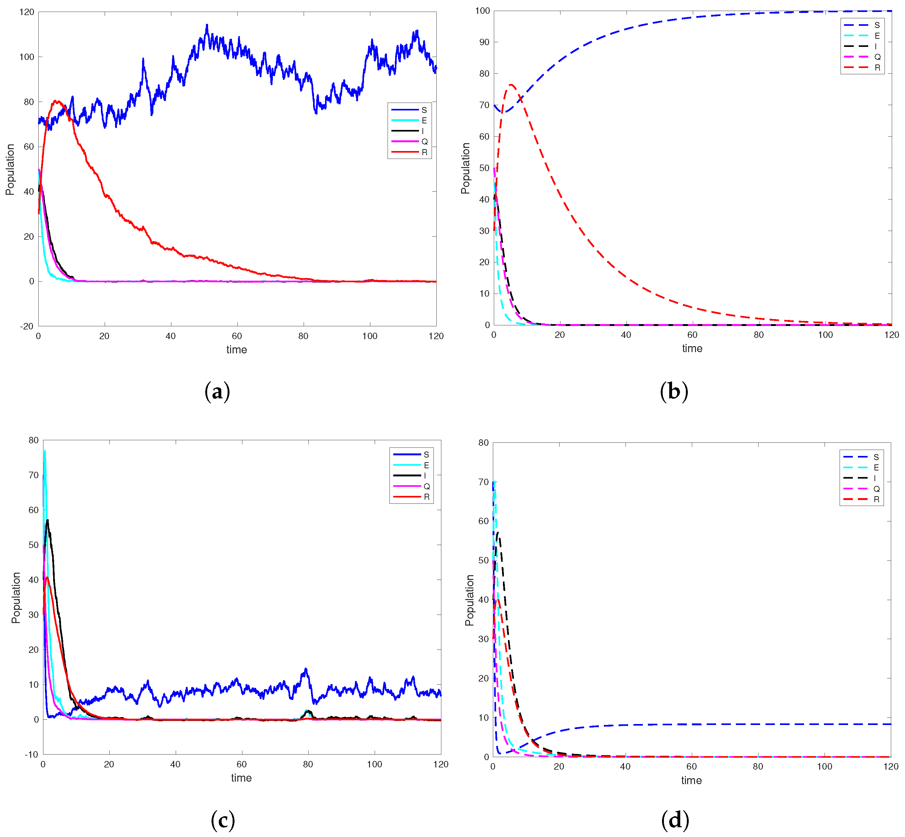
6.1. Simulation Studies on Epidemic Extinction

The previously derived analytical results emphasize that ${\mathcal{R}}_0^E$ is a key threshold value. When ${\mathcal{R}}_0^E$ is less than one, the part of the infected population will approach zero in the long run. The numerical validations shown in Figure 2 provide empirical support for Theorem 2, which states that the infections progressively and consistently depart from the system when ${\mathcal{R}}_0^E<1$. Figure 2a–d show this observation based on the first experiment.

Table 2. Values of the parameters for simulating the models.

Parameters	Case 1	Case 2	Case 3	Source
$\mathrm{\Pi }$	5.00	3.50	3.50	Assumed
$\beta$	0.001	0.50	0.30	Assumed
$\lambda$	0.05	0.01	0.03	Assumed
$\epsilon$	0.50	0.30	0.30	Assumed
$\alpha$	0.05	0.30	0.30	Assumed
${\delta }_1$	0.40	0.20	0.20	Assumed
${\delta }_2$	0.20	0.30	0.30	Assumed
$\gamma$	0.50	0.40	0.10	Assumed
${\eta }_1$	0.50	1.50	0.67	Assumed
${\eta }_2$	0.60	1.40	0.59	Assumed
${\eta }_3$	0.50	1.20	0.50	Assumed
${\eta }_4$	0.21	1.32	0.45	Assumed
${\eta }_5$	0.19	1.20	0.50	Assumed
$\mathsf{S}\left(t\right)$	70.0	70.0	7.00	Assumed
$\mathsf{E}\left(t\right)$	50.0	50.0	5.00	Assumed
$\mathsf{I}\left(t\right)$	40.0	40.0	4.00	Assumed
$\mathsf{Q}\left(t\right)$	50.0	50.0	5.00	Assumed
$\mathsf{R}\left(t\right)$	50.0	50.0	3.00	Assumed

(Case 1) displays the system’s parameters and the corresponding initial values of the states of the model (2). Figure 2 shows that the reproduction number ${\mathcal{R}}_0^E$ serves as the critical value for the infection elimination from the population aligned with the system (1). Furthermore, by restricting the corresponding threshold of the stochastic model (2), the associated solution will fluctuate around the DFE of the ODE model, reflecting the elimination of NoV. The simulation is performed with the help of MATLAB R2017a to investigate the dynamics of the models under various settings. To conclude this preeminent, we can say that both Theorem 2 and our simulations in Figure 2 agree upon disease extinction whenever the reproduction number satisfies the relation ${\mathcal{R}}_0^E\le 1$, which is the main aim of this subsection.

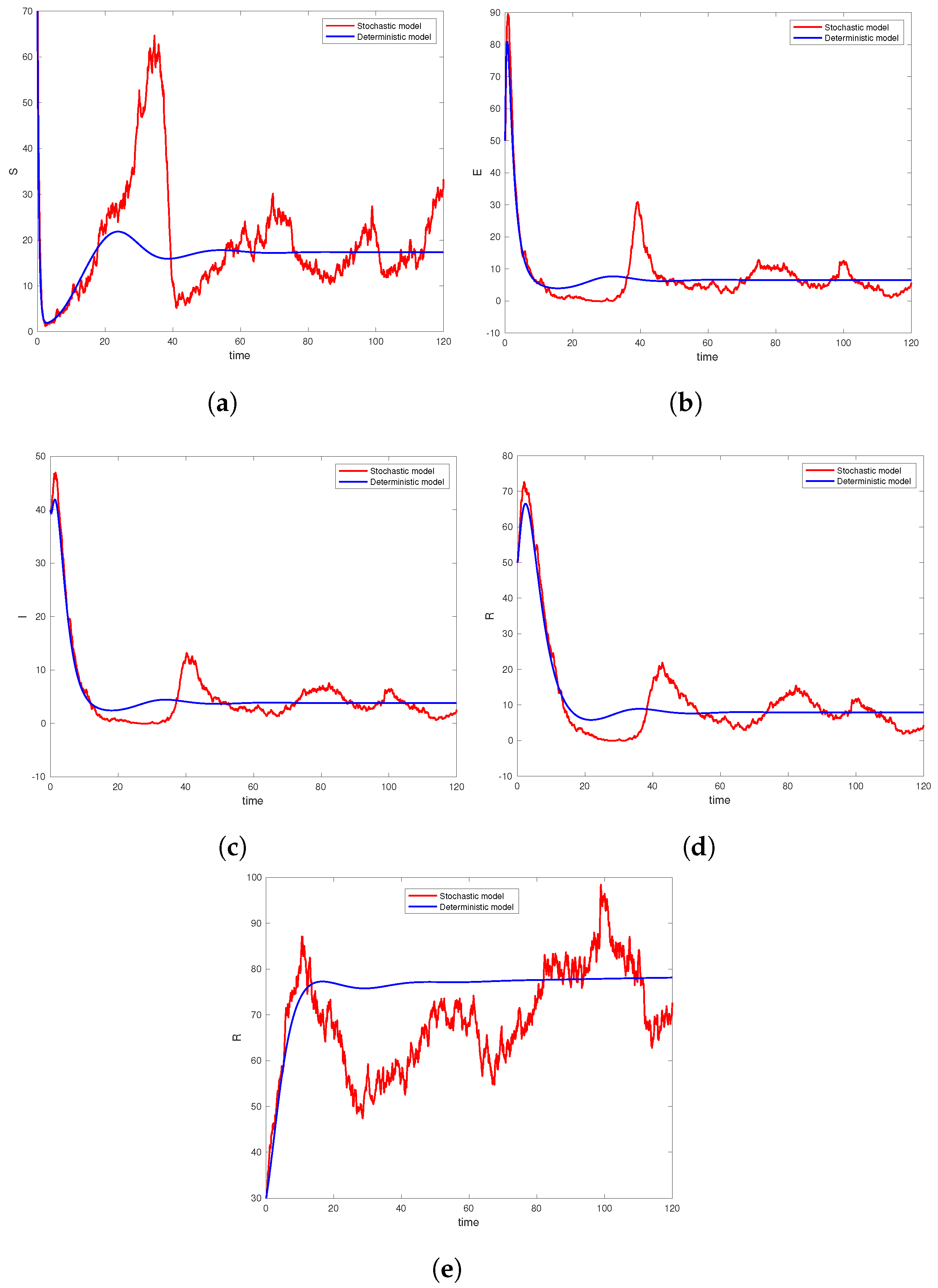
6.2. Numerical Analysis of Ergodicity and Stationary Distribution

The analytical results from the permanence of the infection, and particularly Theorem 3, provide evidence of showing infection in the community at all times when the threshold quantity exceeds unity. After adjusting the values of the parameters, we found that ${\widehat{\mathcal{R}}}_s$ is greater than one. Keeping in view this setting, we simulated the models and observed that the total number of infected nodes remains non-negative and finally stabilizes over time to a nontrivial value. Thus, as suggested by Theorem 3, the infection is likely to remain in the population. The simulations investigate infection dynamics in the population, taking into account both geographical and temporal aspects. Table 2 (Case 2) presents the parameters and initial values of the variables associated with the system (2). Theorem 3 suggests that the infection may persist within the community, provided the model (2) effectively reflects the dynamics of NoV as illustrated in Figure 3a–e. The stochastic model’s reproductive value ${\widehat{\mathcal{R}}}_s$ is more than one, suggesting possible persistence, while the ODE model’s threshold also exceeds one as illustrated in Figure 3. Table 2 (Case 3) shows the initial values of the variables and parameters associated with the model (2). Here again, the threshold quantities are greater than one. The results demonstrate that the stochastic model captures fluctuations in the exposed class more effectively than the deterministic model, reflecting the impact of environmental noise on disease transmission dynamics. The exposed class shows significant variability, emphasizing the importance of considering stochastic influences in understanding real-world norovirus outbreaks. However, we have changed the intensities of the white noises, and as a result, the dynamics of the model have changed drastically. The intensity of the noises has a direct impact on the dynamic behavior of the solution trajectories as suggested by Figure 4a–e. The analysis of the infected class indicates that the inclusion of stochastic elements results in higher amplitude oscillations compared to the deterministic counterpart. This suggests that random environmental factors can substantially alter the infection rate, reinforcing the need for stochastic modeling in capturing the unpredictability of norovirus transmission.

The observed disparity between the mean trajectories of the stochastic and deterministic models arises primarily due to the magnitude of stochastic perturbations incorporated in our simulations. In the stochastic framework, the independent injection of white noise into each compartment induces stochastic variability, which inherently diverges from the smooth dynamics governed by the deterministic model. As the amplitude of these stochastic perturbations diminishes, we anticipate an asymptotic convergence of the stochastic trajectories towards their deterministic counterparts. The current results exemplify how stochastic environmental fluctuations can introduce significant deviations from deterministic predictions, underscoring the impact of noise intensity on the system’s dynamic behavior.

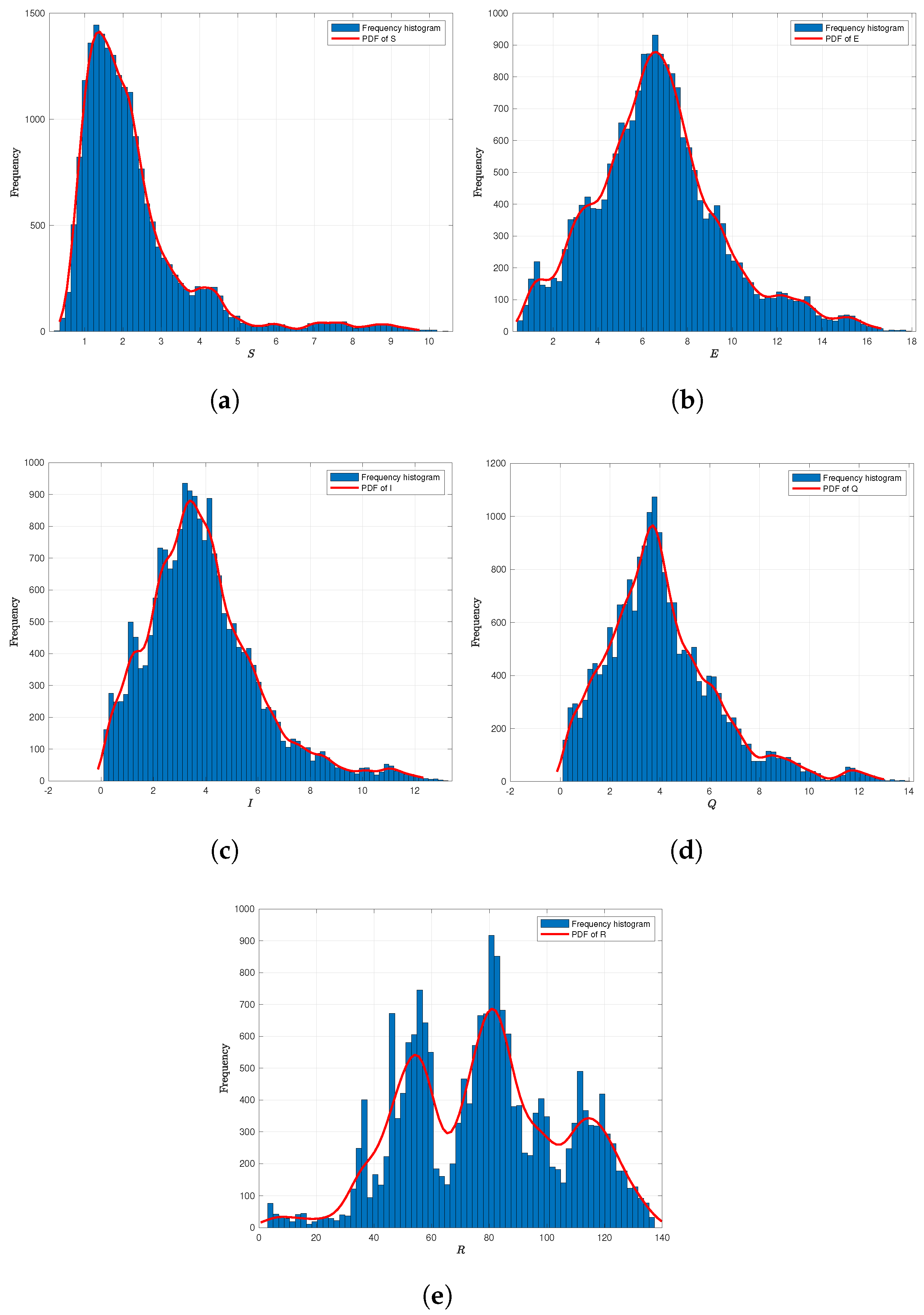
Frequency Histogram of System (2)

To provide a thorough study of how each individual noise component affects the dynamic response of the system (2), we assume that the system is impacted by only one stochastic noise source. Figure 5a–e show how noise intensity affects the variations within each group. These figures are produced using the initial conditions and parameters of the system (2) from Table 2 (Case 3). The finding demonstrates that low-intensity noise causes minor variations in the respective population’s curve, but high-intensity noise causes considerable oscillations and keeps populations at particular levels. Histograms display the solutions and the associated curves of the marginal density functions for each population. Figure 5 also indicates the existence of a stationary distribution for the system (2). We ran multiple numerical simulations and gathered the values of the state variables, which are represented in Figure 5a–e. The distributions depicted in these figures stay constant across time, suggesting their stationary property. The figures further show that the form of the stationary distribution gets more prominent as the degree of noise rises.

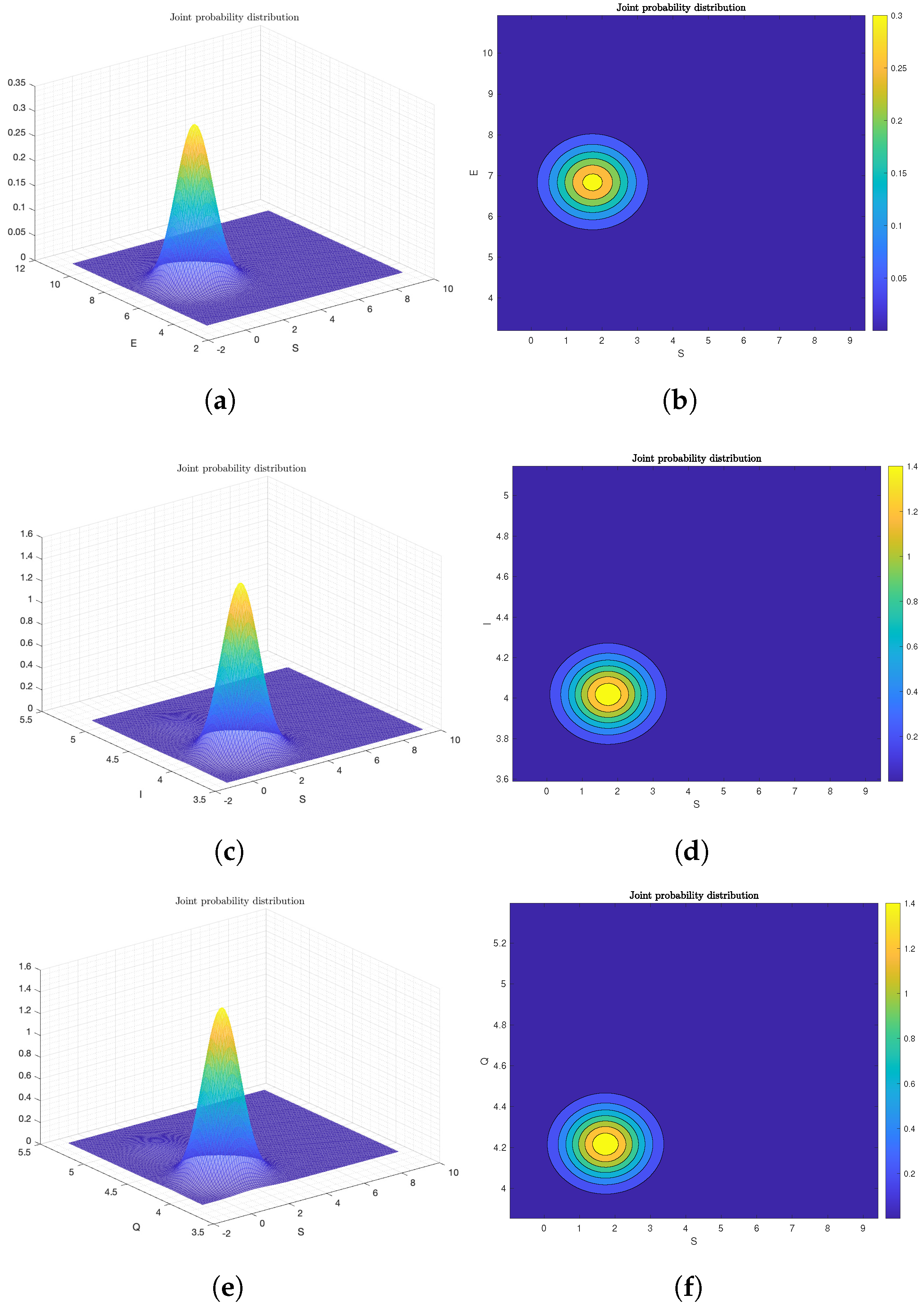
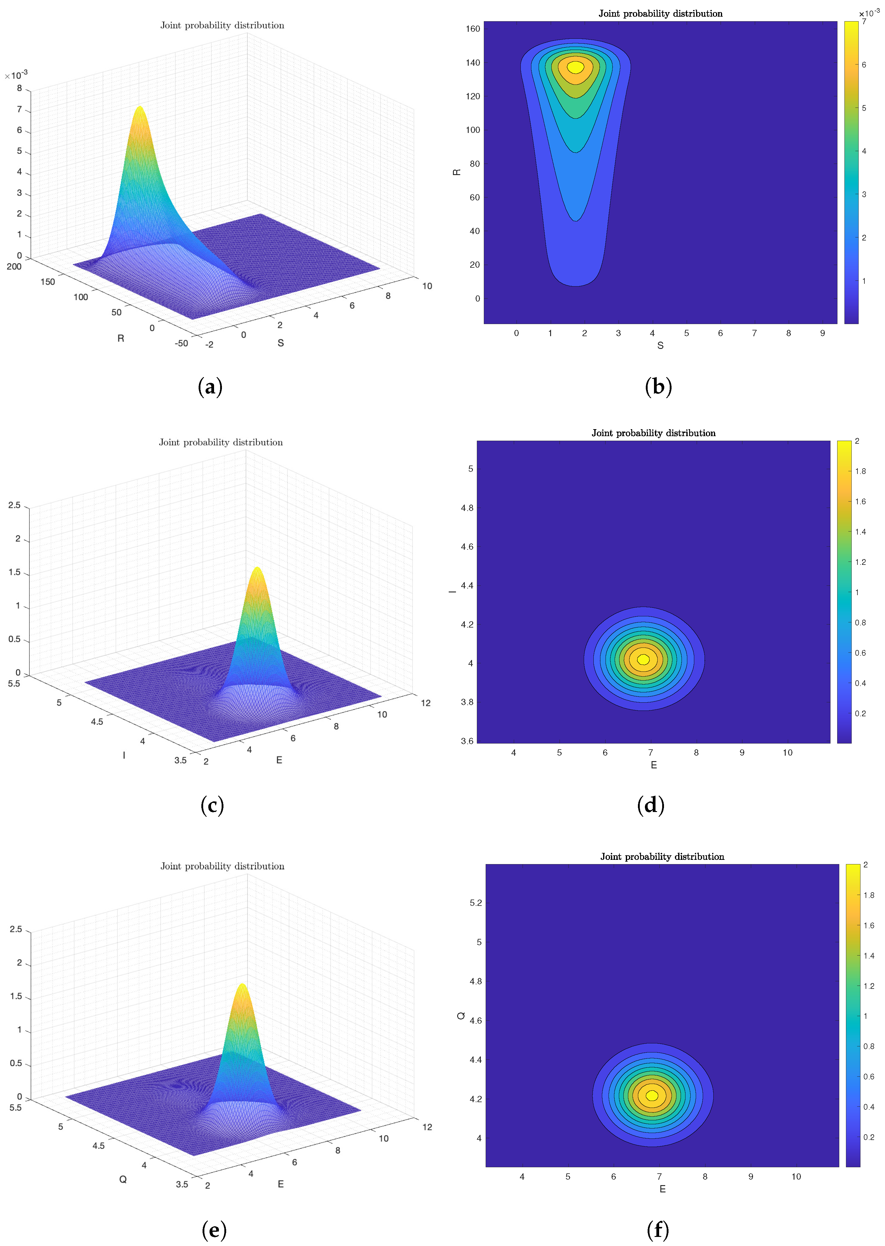
6.3. The Effect of Probability Density Function

In the preceding sub-parts of the simulation, we explored the dynamics of the proposed systems using numerical solution, focusing on the sign transition of the threshold parameter. Now, we will investigate the long-run phenomenological bifurcation (LRP-bifurcation), which is defined by drastic changes in the form of our model’s stationary probability density function. We seek to quantitatively investigate how the parameter $\beta$ affects the form of the probability density function. By closely inspecting Figure 4, we can observe that the transmission parameter $\beta$ has a substantial impact on the support and form of the stationary distribution for model (2). As the value of $\beta$ decreases from $1.98$ to $1.05$, the support of the density function changes remarkably. Higher values of $\beta$ produce stochastic trajectories with significant fluctuations and leaps. Smaller $\beta$ values lead to stochastic trajectories that cluster around the endemic equilibrium as demonstrated in Figure 6 and Figure 7 (Figure 6a–f and Figure 7a–f).

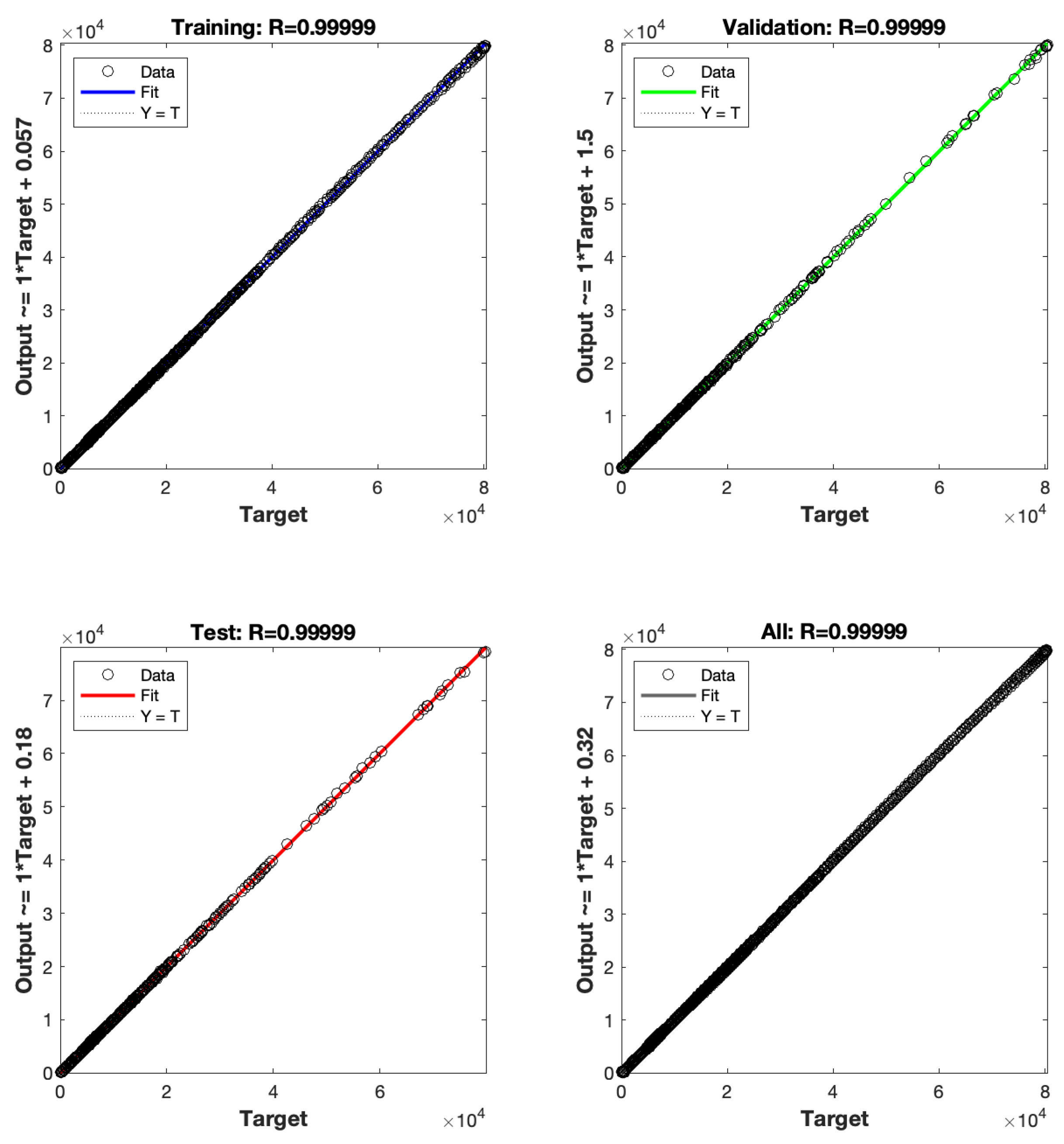
6.4. The LMBNNs Method

The Levenberg–Marquardt backpropagation neural network (LMBNN) algorithm is used to address the dynamic behavior of the stochastic model outlined in system (2), and biologically describe the transmission of the stochastic kind of norovirus (SKNov) system. The scheme is developed and employed for three components of the model (that is, $\mathsf{S},\mathsf{I}$, and $\mathsf{Q}$), and the results are shown in Figure 8a,c,d. These images depict the SKNov system’s workflow diagram, which shows the design in two separate metrics: LMBNNs-based processes and mathematical processes. The dataset design uses the Adam technique, with data divided into 82% for training and 9% for verification as stated in Table 2 (Case 3). For the analysis of the hidden layers, we use the log-sigmoid transfer function, and a single input–output layer structure (based on neurons) is formulated. The present neural network investigation is being undertaken with great care to address concerns such as untimely conjunction, overfitting, and concealed situations. As a result, the network parameters have been carefully chosen following experience, significant testing, and understanding. Fine-tuning of the parameter settings is performed with great accuracy, as minor changes can dramatically affect the entire scenario and damage the investigation’s performance. In the MATLAB program, we utilize the NFTOOL command to run the stochastic process based on LMBNNs, ensuring accurate hidden neuron section configurations, testing statistics, learning methods, and validation statistics. Table 2 shows the parameter settings used to solve the SKNov model using LMBNNs. The SKNov model’s performance is assessed using mean square error (MSE) and state evolution (SE) as shown in Figure 8. Figure 9 shows the regression results for Case 3 in Table 2, with a computed value of one indicating a perfect model.

7. Conclusions and Future Research Directions

In conclusion, this research discussed the substantial worldwide impact of norovirus, a primary cause of viral gastroenteritis notorious for its death, morbidity, and healthcare expenditures. The already established models for NoV assume the mass action law $f\left(I\right)=\beta I$ and saturation law $\left(f\left(I\right)={\displaystyle \frac{\beta I}{1+aI}}\right)$ which have many shortcomings. Therefore, we focused on developing and analyzing a stochastic $\mathsf{S}\mathsf{E}\mathsf{I}\mathsf{Q}\mathsf{R}$ epidemic model that included temporal immunity and a generalized incidence rate. We proved the existence of a single positive global solution by rigorously analyzing the problem. We also explored the extinction dynamics of the $\mathsf{S}\mathsf{E}\mathsf{I}\mathsf{Q}\mathsf{R}$ epidemic model, studying its ergodicity and equilibrium distribution using Khasminskii’s technique and Lyapunov function theory. Our study indicated that the system has a unique ergodic stationary distribution when ${\widehat{\mathcal{R}}}_s>1$, and the property of extinction of the disease when ${\mathcal{R}}_0^E<1$. Numerical simulations corroborated these theoretical conclusions, highlighting the importance of noise intensity in epidemic propagation dynamics. We used the Milstein approach to simulate the stochastic model, whereas the RK4 method was used to solve the corresponding ODE system. We presented example curves for the ODE model and compared the findings to the predictions obtained from the stochastic model. Our study helps in comprehending chronic infectious illnesses on a worldwide scale, with a special emphasis on norovirus. The simulation found that NoV spread through contaminated water and food is more significant than human-to-human spread, reducing the likelihood of cross-contamination. Our focus on the stationary distribution of epidemic models, particularly those with nonlinear stochastic disturbances, highlights the relevance of the approaches in developing the Lyapunov functions.

Table 3. Comparison with previous works.

Citation	Model Type	Major Work	Advancements Offered by Our Model
[44]	Stochastic	Examined environmental and direct transmissions.	Our model not only uses advanced simulation techniques for more accurate predictions but also incorporates a generalized incidence function and considers temporal immunity, allowing for a more realistic representation of norovirus transmission dynamics under varying environmental conditions.
[45]	Stochastic	Focused on hand hygiene’s effect in nursing homes.	Expands to include more diverse control strategies and their effectiveness under stochastic disturbances.
[46]	Stochastic	Developed a stochastic model to analyze different transmission routes for norovirus.	Our model further enhances this by incorporating seasonal variations and a broader set of epidemiological data for more accurate predictions.
[47]	Stochastic	Explored stochastic modeling for norovirus control with vaccine implementation.	Our model offers a more detailed consideration of environmental factors and temporary immunity in addition to vaccination strategies.
[48]	Stochastic	Investigated the effects of Levy noise on norovirus transmission dynamics.	Unlike models focusing only on stochastic disturbances, ours integrates these with practical disease control strategies like vaccination.
[49]	Stochastic	Developed a stochastic model for norovirus focusing on transmission through contaminated food and water.	Our model extends by incorporating direct human-to-human interactions and a wider range of environmental influences.

discusses a detailed analysis about the value added by our research.

Several fascinating and unanswered questions demand additional exploration. To begin, investigating the effect of other parameters such as time delay or pulse interference on the model’s properties may provide useful insights. Second, investigating more realistic approaches, such as incorporating the effects of Markov switching or lévy leaps, may improve the model’s applicability. These sections are reserved for future investigation. Furthermore, the authors want to expand their study by including spatial and age factors in the models that describe the dynamics of NoV. Future work will also involve introducing periodic functions to model seasonal variations in transmission rates, as well as considering spatial heterogeneity and population movement to better understand the spread of norovirus in real-world settings.

References

1. Koopmans, M.; Duizer, E. Foodborne viruses: An emerging problem. Int. J. Food Microbiol. 2004, 90, 23–41. [Google Scholar] [CrossRef] [PubMed]
2. Widdowson, M.A.; Sulka, A.; Bulens, S.N.; Beard, R.S.; Chaves, S.S.; Hammond, R.; Salehi, E.D.P.; Swanson, E.; Totaro, J.; Woron, R.; et al. Norovirus and foodborne disease, United States, 1991–2000. Emerg. Infect. Dis. 2005, 11, 95–102. [Google Scholar] [CrossRef] [PubMed]
3. Mokhtari, A.; Jaykus, L.A. Quantitative exposure model for the transmission of norovirus in retail food preparation. Int. J. Food Microbiol. 2009, 133, 38–47. [Google Scholar] [CrossRef] [PubMed]
4. Bean, N.H.; Goulding, J.S.; Daniels, M.T.; Angulo, F.J. Surveillance for foodborne disease outbreaks—United States, 1988–1992. J. Food Prot. 1997, 60, 1265–1286. [Google Scholar] [CrossRef] [PubMed]
5. Ahmed, S.M.; Lopman, B.A.; Levy, K. A systematic review and meta-analysis of the global seasonality of norovirus. PLoS ONE 2013, 8, e75922. [Google Scholar] [CrossRef]
6. Marshall, J.A.; Bruggink, L.D. The dynamics of norovirus outbreak epidemics: Recent insights. Int. J. Environ. Res. Public Health 2011, 8, 1141–1149. [Google Scholar] [CrossRef]
7. Rohayem, J. Norovirus seasonality and the potential impact of climate change. Clin. Microbiol. Infect. 2009, 15, 524–527. [Google Scholar] [CrossRef]
8. Carmona-Vicente, N.; Fernández-Jiménez, M.; Ribes, J.M.; Téllez-Castillo, C.J.; Khodayar-Pardo, P.; Rodríguez-Diaz, J.; Buesa, J. Norovirus infections and seroprevalence of genotype GII. 4-specific antibodiesin a Spanish population. J. Med. Virol. 2015, 87, 675–682. [Google Scholar] [CrossRef]
9. Honma, S.; Nakata, S.; Numata, K.; Kogawa, K.; Yamashita, T.; Oseto, M.; Jiang, X.; Chiba, S. Epidemiological study of prevalence of genogroup II human calicivirus (Mexico virus) infections in Japan and Southeast Asia as determined by enzyme- linked immunosorbent assays. J. Clin. Microbiol. 1998, 36, 2481–2484. [Google Scholar] [CrossRef]
10. Simmons, K.; Gambhir, M.; Leon, J.; Lopman, B. Duration of immunity to norovirus gastroenteritis. Emerg. Infect. Dis. 2013, 19, 1260–1267. [Google Scholar] [CrossRef]
11. Hall, A.J.; Lopman, B.A.; Payne, D.C.; Patel, M.M.; Gastañaduy, P.A.; Vinjé, J.; Parashar, U.D. Norovirus disease in the United States. Emerg. Infect. Dis. 2013, 19, 1198–1205. [Google Scholar] [CrossRef] [PubMed]
12. Lai, C.C.; Wang, Y.H.; Wu, C.Y.; Hung, C.H.; Jiang, D.D.S.; Wu, F.T. A norovirus outbreak in a nursing home: Norovirus shedding time associated with age. J. Clin. Virol. 2013, 56, 96–101. [Google Scholar] [CrossRef]
13. Murata, T.; Katsushima, N.; Mizuta, K.; Muraki, Y.; Hongo, S.; Matsuzaki, Y. Prolonged norovirus shedding in infants 6 months of age with gastroenteritis. Pediatr. Infect. Dis. J. 2007, 26, 46–49. [Google Scholar] [CrossRef]
14. Din, A.; Li, Y.; Khan, T.; Zaman, G. Mathematical analysis of spread and control of the novel corona virus (COVID-19) in China. Chaos Solitons Fractals 2020, 141, 110286. [Google Scholar] [CrossRef]
15. Khan, F.M.; Khan, Z.U. Numerical Analysis of Fractional Order Drinking Mathematical Model. J. Math. Tech. Model. 2024, 1, 11–24. [Google Scholar]
16. Gaythorpe, K.A.M.; Trotter, C.L.; Lopman, B.; Steele, M.; Conlan, A.J.K. Norovirus transmission dynamics: A modelling review. Epidemiol. Infect. 2018, 146, 147–158. [Google Scholar] [CrossRef] [PubMed]
17. Liu, G.; Qi, H.; Chang, Z.; Meng, X. Asymptotic stability of a stochastic May mutualism system. Comput. Math. Appl. 2020, 79, 735–745. [Google Scholar] [CrossRef]
18. Tran, K.Q.; Yin, G. Optimal harvesting strategies for stochastic ecosystems. IET Control. Theory Appl. 2017, 11, 2521–2530. [Google Scholar] [CrossRef]
19. Ma, T.; Meng, X.; Chang, Z. Dynamics and optimal harvesting control for a stochastic one-predator-two-prey time delay system with jumps. Complexity 2019, 2019, 5342031. [Google Scholar] [CrossRef]
20. Din, A. The stochastic bifurcation analysis and stochastic delayed optimal control for epidemic model with general incidence function. Chaos 2021, 31, 31. [Google Scholar] [CrossRef]
21. Huo, L.A.; Dong, Y.F.; Lin, T.T. Dynamics of a stochastic rumor propagation model incorporating media coverage and driven by Lévy noise. Chin. Phys. B 2021, 30, 080201. [Google Scholar] [CrossRef]
22. Din, A.; Li, Y. Lévy noise impact on a stochastic hepatitis B epidemic model under real statistical data and its fractal–fractional Atangana–Baleanu order model. Phys. Scr. 2021, 96, 124008. [Google Scholar] [CrossRef]
23. Wang, L.L.; Huang, N.J. Ergodic stationary distribution of a stochastic nonlinear epidemic model with relapse and cure. Appl. Anal. 2020, 101, 2652–2668. [Google Scholar] [CrossRef]
24. Lopman, B.; Simmons, K.; Gambhir, M.; Vinjé, J.; Parashar, U. Epidemiologic implications of asymptomatic reinfection: A mathematical modeling study of norovirus. Am. J. Epidemiol. 2013, 179, kwt287. [Google Scholar] [CrossRef]
25. Vanderpas, J.; Louis, J.; Reynders, M.; Mascart, G.; Vandenberg, O. Mathematical model for the control of nosocomial norovirus. J. Hosp. Infect. 2009, 71, 214–222. [Google Scholar] [CrossRef] [PubMed]
26. Lee, R.M.; Lessler, J.; Lee, R.A.; Rudolph, K.E.; Reich, N.G.; Perl, T.M.; Cummings, D.A. Incubation periods of viral gastroenteritis: A systematic review. BMC Infect. Dis. 2013, 13, 1. [Google Scholar] [CrossRef] [PubMed]
27. Khan, W.A.; Zarin, R.; Zeb, A.; Khan, Y.; Khan, A. Navigating Food Allergy Dynamics via a Novel Fractional Mathematical Model for Antacid-Induced Allergies. J. Math. Tech. Model. 2024, 1, 25–51. [Google Scholar]
28. Anderson, R.M.; May, R.M. Infectious Disease of Humans: Dynamics and Control; Oxford University Press: Oxford, UK, 1991. [Google Scholar]
29. Li, L.; Bai, Y.P.; Jin, Z. Periodic solutions of an epidemic model with saturated treatment. Nonlinear Dyn. 2014, 76, 1099–1108. [Google Scholar] [CrossRef]
30. Zhang, Z.H.; Suo, Y.H. Qualitative analysis of a SIR epidemic model with saturated treatment rate. Appl. Math. Comput. 2010, 34, 177–194. [Google Scholar]
31. Ebert, D.; Zschokke-Rohringer, C.D.; Carius, H.J. Dose effects and density-dependent regulation of two microparasites of Daphnia magna. Oecologia 2000, 122, 200–209. [Google Scholar] [CrossRef]
32. Song, X.Y.; Neumann, A.U. Global stability and periodic solution of the viral dynamics. J. Math. Anal. Appl. 2007, 329, 281–297. [Google Scholar] [CrossRef]
33. Anderson, R.M.; May, R.M. Regulation and stability of host-parasite population interactions: I. Regulatory processes. J. Anim. Ecol. 1978, 47, 219–247. [Google Scholar] [CrossRef]
34. Din, A.; Li, Y. Optimizing HIV/AIDS dynamics: Stochastic control strategies with education and treatment. Eur. Phys. J. Plus 2024, 139, 1–19. [Google Scholar] [CrossRef]
35. Caraballo, T.; Fatini, M.E.; Pettersson, R.; Taki, R. A stochastic SIRI epidemic model with relapse and media coverage. Discrete Contin. Dyn. Syst. Ser. B 2018, 23, 2483–3501. [Google Scholar] [CrossRef]
36. Chen, X.Y.; Cao, J.D.; Park, J.H.; Qiu, J.L. Stability analysis and estimation of domain of attraction for the endemic equilibrium of a SEIQ epidemic model. Nonlinear Dyn. 2017, 87, 975–985. [Google Scholar] [CrossRef]
37. Fan, K.G.; Zhang, Y.; Gao, S.J.; Wei, X. A class of stochastic delayed SIR epidemic models with generalized nonlinear incidence rate and temporary immunity. Physica A 2017, 481, 198–208. [Google Scholar] [CrossRef]
38. El Fatini, M.; El Khalifi, M.; Gerlach, R.; Laaribi, A.; Taki, R. Stationary distribution and threshold dynamics of a stochastic SIRS model with a general incidence. Phys. A Stat. Mech. Its Appl. 2019, 534, 120696. [Google Scholar] [CrossRef]
39. Liu, Q.; Jiang, D.Q.; Hayat, T.; Alsaedi, A.; Ahmad, B. A stochastic SIRS epidemic model with logistic growth and general nonlinear incidence rate. Physica A 2020, 551, 124152. [Google Scholar] [CrossRef]
40. Zhang, Y.; Ma, X.; Din, A. Stationary distribution and extinction of a stochastic SEIQ epidemic model with a general incidence function and temporary immunity. AIMS Math 2021, 6, 12359–12378. [Google Scholar] [CrossRef]
41. Zhao, Y.N.; Jiang, D.Q. The threshold of a stochastic SIS epidemic model with vaccination. Appl. Math. Comput. 2014, 243, 718–727. [Google Scholar] [CrossRef]
42. Khasminskii, R. Stochastic Stability of Differential Equations; Springer: Berlin/Heidelberg, Germany, 2012. [Google Scholar]
43. Higham, D.J. An algorithmic introduction to numerical simulation of stochastic differential equations. SIAM Rev. 2001, 43, 525–546. [Google Scholar] [CrossRef]
44. Towers, S.; Chen, J.; Cruz, C.; Melendez, J.; Rodriguez, J.; Salinas, A.; Yu, F.; Kang, Y. Quantifying the relative effects of environmental and direct transmission of norovirus. R. Soc. Open Sci. 2018, 5, 170602. [Google Scholar] [CrossRef] [PubMed]
45. Assab, R.; Temime, L. The role of hand hygiene in controlling norovirus spread in nursing homes. BMC Infect. Dis. 2016, 16, 395. [Google Scholar] [CrossRef] [PubMed]
46. Rushton, S.P.; Sanderson, R.A.; Reid, W.D.; Shirley, M.D.; Harris, J.P.; Hunter, P.R.; O’Brien, S.J. Transmission routes of rare seasonal diseases: The case of norovirus infections. Philos. Trans. R. Soc. B 2019, 374, 20180267. [Google Scholar] [CrossRef] [PubMed]
47. Din, A. Optimal control theory of a novel stochastic human norovirus model and vaccine development. Int. J. Mod. Phys. B 2022, 36, 2250238. [Google Scholar] [CrossRef]
48. Cui, T.; Din, A.; Liu, P.; Khan, A. Impact of Levy noise on a stochastic Norovirus epidemic model with information intervention. Comput. Methods Biomech. Biomed. Eng. 2023, 26, 1086–1099. [Google Scholar] [CrossRef]
49. Din, A.; Li, Y. Stochastic optimal control for norovirus transmission dynamics by contaminated food and water. Chin. Phys. B 2022, 31, 020202. [Google Scholar] [CrossRef]
Figure 1. Structure and life cycle of norovirus.
Fractalfract 08 00586 g001
Figure 2. Comparison between the paths of stochastic (2) and deterministic (1) systems when the respective threshold parameters are less and greater than one. (a) Stochastic model’s path for threshold < 1 . (b) Deterministic model’s path for R 0 < 1 . (c) Stochastic model’s path for threshold > 1 . (d) Deterministic model’s path for R 0 > 1 .
Fractalfract 08 00586 g002
Figure 3. The plot shows numerical simulations of the stochastic model (2) and deterministic system (1) when R ^ s > 1 with very small values of the white noises. The model has a distinctive ergodic stationary distribution, implying a persistent infection. (a) Susceptible class. (b) Exposed class. (c) Infected class. (d) Quarantined class. (e) Recovered class.
Fractalfract 08 00586 g003
Figure 4. The graphic shows numerical simulations of the stochastic model (2) and the deterministic system (1) when R ^ s > 1 and there are strong white noises. Again, the model shows a unique ergodic stationary distribution, indicating chronic infection with a larger amplitude. (a) Susceptible class. (b) Exposed class. (c) Infected class. (d) Quarantined class. (e) Recovered class.
Fractalfract 08 00586 g004
Figure 5. Frequency histograms of all compartments obtained from several simulations with different intensities of white noises. (a) Susceptible class. (b) Exposed class. (c) Infected class. (d) Quarantined class. (e) Recovered class.
Fractalfract 08 00586 g005
Figure 6. The right panel of the figure shows the combined two-dimensional densities of the compartments S , E , I , and Q obtained from system (2) at t = 1000 . The frequency histograms are constructed with N = 100,000 simulation trials as shown in Table 2 (Case 3). Different colors signify different density sizes. The left panel shows a 3D graph displaying the two-dimensional densities of the stated compartments. (a) S and E Joint Probability Distribution (left). (b) S and E Joint Probability Distribution (right). (c) S and I Joint Probability Distribution (left). (d) S and I Joint Probability Distribution (right). (e) S and Q Joint Probability Distribution (left). (f) S and Q Joint Probability Distribution (right).
Fractalfract 08 00586 g006
Figure 7. The figure’s right panel shows the combined two-dimensional densities of the classes S , E , and R in system (2) at t = 1000. The frequency histograms were constructed using N = 100,000 simulation trials as shown in Table 2. Different colors denote different density sizes. The left panel shows a 3D graph with the two-dimensional combined densities of S , E , and R . (a) S and R Joint Probability Distribution (left). (b) S and R Joint Probability Distribution (right). (c) E and I Joint Probability Distribution (left). (d) E and I Joint Probability Distribution (right). (e) E and Q Joint Probability Distribution (left). (f) E and Q Joint Probability Distribution (right).
Fractalfract 08 00586 g007
Figure 8. MSE and STs for the SKNov system (2). (a) Population dynamics of various compartments over time. (b) Error histogram showing distribution of training, validation, and test errors. (c) Function fit and error plot for the network output. (d) Mean squared error (MSE) over training epochs, highlighting the best validation performance.
Fractalfract 08 00586 g008
Figure 9. Regression analysis of the SKNov system (2).
Fractalfract 08 00586 g009